Investments under vertical relations and agency con‡icts: a real options approach Dimitrios Zormpas August 22, 2018
Abstract We examine the case of a …rm holding the option to make an uncertain and irreversible investment. The …rm is decentralized and there is information asymmetry between the owner and the investment manager regarding the price of an input (e.g. a key equipment) that needs to be purchased by an outside supplier with market power. We show that the total loss attributed to the information asymmetry has two components: i) the loss in the decentralized …rm itself and ii) a negative externality that the outside input supplier endures. We show that the latter is likely not just a part, but rather the main component of the total loss. Last, we prove that the negative externality is reduced when the principal uses an audit technology in parallel with the bonus-incentive mechanism. keywords: Real options, Vertical relations, Asymmetric information, Agency con‡icts, Audit jel classification: D82, L10.
1
Introduction
The real options approach is a standard framework for the analysis of investment opportunities. It builds on the idea that the option to undertake an investment project is analogous to an American call option on a real asset. Hence, when evaluating an investment option characterized by uncertainty and irreversibility, the potential investor needs to factor in that at the time of the investment s/he forgoes the option to reconsider the investment decision at some future time point when the uncertainty will be, naturally, partly resolved.1 The standard real options model does not account for agency con‡icts and information asymmetries since the investment is assumed to be managed by the potential investor her/himself. However, in many modern corporations, investment decisions are delegated by the owner of the corporation (principal) to a manager (agent) who possesses a relevant skill set or piece of information.2 Of course the principal bene…ts from the expertise of the agent but, at the same time, s/he might be exposed to information asymmetries. If the agent has an informational advantage over the principal, then the latter must carefully consider the underlying motives when deciding the terms of the Department of Mathematics, University of Padova, Via Trieste 63, 35121, Padova, Italy. Email:
[email protected]. 1 See Dixit and Pindyck (1994) and Trigeorgis (1996) for an overview of the real options approach. 2 Delegation is a standard practice when managing large enterprises (Amaral et al., 2006). For relevant examples from industries that have to do with textiles, construction, aeronautics, telecommunications, computers, automobiles, electronics and business services, see e.g. Agrell et al. (2004), Lee et al. (2004), Schieg (2008), Tang et al. (2009), Deshpande et al. (2011), Doorey (2011), Kayis et al. (2013), Bolandifar et al. (2016), Agrell and Bogetoft (2017) and Dietrich et al. (2008).
1
delegation. More precisely, the principal needs to develop an appropriate mechanism in order to incentivize the agent to share private information resolving the information asymmetry. The use of such a mechanism is costly for the principal but, without it, s/he is due to face further distortions stemming from the coordination failure.3 As we will see in the next section, there is a growing body of papers that incorporate agency con‡icts that stem from information asymmetries into the real options model. In spite of the di¤erences in their analyses, what these papers share is the assumption that the investment cost is exogenous. As Billette de Villemeur et al. (2014) point out, this assumption is sensible when an investment is performed largely in-house as, for instance, in a research and development project. Nevertheless, this is not always true. Investment projects are often rather complex and specialized inputs might be needed.4 At the same time, the potential investor might lack the equipment and/or the expertise to manufacture the needed input. In these cases, the investment cost is endogenous since it is speci…ed by the vertical relationship between the external input supplier and the potential investor. For instance, Billette de Villemeur et al. refer to investments in the vaccine industry where facilities are speci…cally designed for the production of a novel vaccine. In this case, the needed customized equipment is sourced on an intermediate market from input providers with market power. Similarly, Pennings (2017) refers to large infrastructure projects as, e.g., a telecommunications network. In that case, an upstream …rm (construction company) is responsible for the provision of an indispensable input (network), to a downstream …rm (internet provider). The key originality of this paper lies in the combination of the decentralized investment setting with the endogenous pricing of a necessary input. Using the real options approach, we examine the case of a potential investor who is contemplating making an uncertain investment. A prerequisite for the investment to take place is the provision of a specialized input by an external supplier with market power. Since the input is relationship-speci…c, i) the investment cost is sunk and ii) the principal delegates the investment decision to an agent with a relevant expertise.5 Our …ndings suggest the following: First, we show that the presence of an external input supplier with market power, makes the investment more expensive, favoring its postponement while reducing the value of the option to invest. Second, we show that the total losses attributed to the resolution of the agency con‡ict in the …rm, can be decomposed into two components: i) the loss in the decentralized …rm and ii) the negative externality that the input supplier endures when s/he fails to anticipate the agency con‡ict downstream. The …rst component of the total social loss is already analyzed in detail in the literature. However, the second component has attracted, to the best of our knowledge, no attention. The two components di¤er in nature in the sense that the …rst one captures the in-…rm cost of using a mechanism to resolve the agency con‡ict whereas, the second one, captures the loss for another …rm in the supply chain, in this case an input supplier, who cannot foresee the incentive misalignment downstream. Moreover, we derive a condition under which the second component is larger than the …rst one and we show that, unless certain parameters obtain extreme values, this condition holds. Last, we show that when the principal resolves the agency con‡ict complementing the standard bonus-incentive mechanism with an audit technology, the negative externality is signi…cantly reduced thanks to a reduction in the relevant timing distortion. 3
For an overview of the literature on asymmetric information see e.g. La¤ont and Martimort (2002). See e.g., Agrell and Bogetoft (2017), Hargadon and Sutton (2000) and Linder (2004). 5 The agent might have specialized information related to the input (Mookherjee and Tsumagari, 2004), or s/he might be responsible for the solution of a matching problem if direct communication between the project originator and the input supplier is impossible, or prohibitively expensive (Faure-Grimaud and Martimort, 2001). Alternatively, the agent might just be what Hayek (1945) calls the "person on the spot". For instance, McAfee and McMillan (1995) assume that the principal opts for disintegration when the management of the project takes time and the principal’s time is limited. Similarly, Van Zandt (1999) argues that the need for delegation might stem from the …xed information processing capacity of the principal. 4
2
The remainder of the paper is organized as follows. In Section 2 we present an overview of the related literature. In Section 3 we present in detail the model set-up demonstrating the connections with previous work. In Section 4 we analyze the total loss that is attributable to the information asymmetry between the principal and the agent. In Section 5 we discuss the agency con‡ict when an audit technology is used. In Section 6 we present some numerical examples whereas in Section 7 we discuss the special case of supply chains characterized by traceability and transparency. Section 8 concludes.
2
Overview of the related literature
This work contributes to the research area that integrates the basic theory of irreversible investment under uncertainty as e.g. in Dixit and Pindyck (1994) and the literature on asymmetric information as e.g. in La¤ont and Martimort (2002).6 Grenadier and Wang (2005) analyze the timing and e¢ ciency of an investment undertaken in a decentralized setting under the presence of information asymmetries and hidden action between the principal and the agent. They show that the principal can induce the agent both to extend e¤ort and to reveal private information by using a bonus-incentive mechanism. Despite the fact that the use of such an instrument is suboptimal in the sense that the chosen investment timing di¤ers from the timing in the setting with symmetry of information, the principal’s losses are reduced since further distortions are avoided.7 Shibata (2009) extends the analysis presented in Grenadier and Wang (2005) by complementing the bonus-incentive contract with an audit technology. Focusing on the adverse-selection-only case he shows that, by using both auditing and a bonus-incentive, the timing ine¢ ciency is reduced, the principal’s value is larger whereas the agent’s value is smaller. Contributing to the same body of work, Shibata (2008) focuses on the impact of uncertainty on the timing and the value of the project whereas Shibata and Nishihara (2010), Grenadier and Malenko (2011), Morellec and Schürho¤ (2011), Kanagaretnam and Sarkar (2011), Hori and Osano (2014) and Cardoso and Pereira (2015) among others examine the e¤ect of capital structure and …nancing of the investment. Cong (2013) and Bouvard (2014) examine the implications of endogenous learning and experimentation respectively, whereas Mæland (2010) and Koskinen and Mæland (2016) approach the agency con‡ict assuming that the agent is the winner of an auction in which a number of potential delegates participate. Last, Broer and Zwart (2013) examine the optimal regulation of an investment undertaken by a monopolist who has private information on the investment cost whereas Arve and Zwart (2014) examine the case where the information asymmetry between the principal and the agent has to do with the starting point of the process that is used to capture the ‡uctuations of the stochastic parameter. Despite the di¤erences in the adopted framework, what all these papers have in common is the assumption that the investment cost is exogenous. However, as highlighted by Billette de Villemeur et al. (2014), the cost of an investment does not always re‡ect the project’s economic fundamentals. In this work, we apply the endogenous pricing of the input à la Billette de Villemeur et al., in the adverse-selection-only version of the model presented by Grenadier and Wang (2005) and the model 6 We abstain from discussing a related but distinct strand of the literature that analyzes the role of asymmetric information on investments using a static and/or deterministic framework, see e.g., de Wet (2004) and Chen and Liu (2013). 7 In Grenadier and Wang (2005) the management e¤ort is assumed to be exogenous. Shibata and Nishihara (2011) approach the same problem using a two-stage optimization problem that allows investment timing and management e¤ort endogenously decided. The numerical examples that they present suggest that the management e¤ort is greater under asymmetric, than under symmetric, information. This in turn implies that there are trade-o¤s between investment e¢ ciency and management e¤ort under asymmetric information.
3
presented by Shibata (2009), and we discuss the e¤ect of the agency con‡ict downstream on the input supplier upstream and vice versa.
3
The model
In this section we begin with a description of the basic set-up of the model. We then present the integrated case which corresponds to the problem with in-house production of the input, and the separated case, which corresponds to the case where the input is produced by the upstream …rm. Finally, we reapproach the separated case assuming delegation of the investment decision from the project originator to a project manager which is our original contribution.
3.1
The basic set-up
The owner of a …rm, P , holds the option to undertake an investment. In order to do so, P needs a specialized input (e.g. a key equipment) that can be produced in-house (integration) or by an upstream …rm U (separation). The production cost of the input is equal to I and is assumed to be completely sunk. We assume that I can be "low" (Il ) with probability q 2 [0; 1] or "high" (Ih ) with probability 1 q where Ih > Il > 0 and I = Ih Il . Assumption 1: The probability distribution of I is common knowledge whereas the input producer is the only party who observes the true I as soon as this is chosen by Nature. This is a reasonable assumption since the individual with the best information on the production cost is usually the producer her/himself (see e.g., Celik, 2009; Broer and Zwart, 2013). The value of the project is represented by Xt which is assumed to be ‡uctuating over time according to the following geometric Brownian motion: dXt = dt + dzt Xt
(1)
The parameter stands for the positive constant drift, is the positive constant volatility and dzt is the increment of a Wiener process. A lower case x is used to denote the current level of Xt : x = X0 . We assume that P , as the holder of the investment option, can continuously and veri…ably observe the realizations of Xt over time. On the contrary, U knows the structural parameters of process (1) but cannot observe the realizations of Xt at any point in time.8 According to the real options literature, when a potential investor contemplates undertaking an investment characterized by uncertainty and irreversibility, the ability to delay the investment for some future time point is a source of ‡exibility that profoundly a¤ects the decision to invest (see e.g. McDonald and Siegel, 1986). The investment takes place only as soon as the project’s expected payo¤ exceeds the cost of the investment by a margin equal to the option value of further postponing the completion of the project into the future.9 Keeping this in mind, it is assumed throughout the paper that x is su¢ ciently low so that future, rather than immediate, investment is preferred.10 All the parties are assumed to be risk neutral with the risk-free interest rate denoted by r. For convergence we assume r > .11 8
We will analyze the importance of this assumption in subsection 3.3 below. O’Brien et al. (2003), Leahy and Whited (1996) and Guiso and Parigi (1999) present strong empirical evidence supporting this argument. 10 Otherwise the problem reduces to the mere maximization of the net present value. 11 This is a standard assumption. See e.g. Dixit and Pindyck (1994, p. 138). 9
4
3.2
Integrated case
In the integrated case, P produces the needed input in house. S/he is …rst observing the magnitude of I chosen by Nature (Ih or Il ) and is then deciding when to invest. A summary of the timing stages of the integrated case is given in Figure 1. The value of the option to invest is: F (x; X; I) = (X
I)
x X
;
(2)
q 1 2 + 2r2 > 1 is the positive root of the characteristic equation where = 12 + 2 2 2 1 2 ( 1) + r = 0. X denotes a decision variable which is a threshold that, when attained 2 by Xt for the …rst time and from below at a stochastic future date, triggers the investment. The expressions for F (x; X; I) and are standard in the real options literature (see e.g. Dixit and Pindyck, 1994). The value maximizing investment trigger Xi = arg max F (x; X; Ii ) is equal to Xi = 1 Ii and the ex-post value of the option to invest is F (x; Ii ) = I 1 Xx where i 2 fl; hg. The ex-ante i value of the investment option is f = qF (x; Il ) + (1 q) F (x; Ih ). Since > 1, we have = 1 > 1 and Xi > Ii , i 2 fl; hg. The di¤erence between the optimal investment threshold Xi and the sunk investment cost Ii is exactly the margin that is attributed to the uncertainty and the irreversibility characterizing the investment. Note that is decreasing in and whereas it is increasing in r. Consequently, the wedge = 1 is increasing in and whereas it is decreasing in r. Hence, the greater the amount of uncertainty and/or the expected rate of return over the future values of Xt , the larger the excess return that the …rm will demand before it is willing to make the irreversible investment. On the contrary, an increase in the risk-free interest rate r makes waiting costlier for the potential investor.
Figure 1: Integrated Case
3.3
Separated case
Suppose now that the upstream …rm U produces the input. Following the presentation of Billette de Villemeur et al. (2014), we assume for simplicity that the potential investor P is a price-taker in the input market. In this case, U chooses the input price and a vertical distortion between P and U arises. In order to derive the optimal input price and the optimal investment trigger under separation, we begin with the optimization problem of the project originator P . The value of the option to invest for P is x .12 (3) F S (x; X; p) = (X p) X Maximizing we obtain X S (p) = 1 p. Of course this is reminiscent of the optimal investment threshold in the integrated case. Actually, the only di¤erence between the two is the sunk investment 12
The superscript S stands for "separated".
5
cost that P needs to pay for the investment to take place. In the integrated case, the investment cost is equal to the input production cost as this is chosen by Nature, I, whereas in the separated case the investment cost is the price chosen by the input manufacturer U , p. Now, keeping in mind that P will invest as soon as X S (p) is reached, U chooses the optimal price p maximizing her/his option value: K (x; p; I) = (p The optimal price is equal to pi =
1 Ii
I)
x (p)
(4)
XS
which in turn implies XiS =
2 1
Ii =
fl; hg.13 In this case, the ex-post value of the option to invest for P is F S (x; Ii ) = whereas for U we have K (x; Ii ) = for P and U are f S =
1
1
1
1
1 Xi 1
;i 2
F (x; Ii )
F (x; Ii ), i 2 fl; hg. Similarly, the ex-ante option values 1
f and k =
f respectively. Note that f S =
1k
and
lim f S = k. In words, the value of the option to invest is shared in the separated case between P !1
and U , with the lion’s share going always to the holder of the investment option P . The di¤erence between f S and k becomes negligible only when the value of the option to postpone the investment reaches its minimum, i.e., when becomes very large and, consequently, when the wedge = 1 tends to unity. A summary of the timing stages of the separated case is given in Figure 2.
Figure 2: Separated Case
There are two important points to be made here. First, the vertical distortion results in a more expensive investment (pi > Ii ) which is realized, in expected terms, later XiS > Xi ; i 2 fl; hg . This change in the sunk cost of the investment is also re‡ected in the aggregate ex-ante value of the investment option which is lower than the corresponding value in the integrated case: f S + k < f . Second, due to Assumption 1, in the separated case it is U , not P , the party that is observing the true magnitude of I. However, the buyer of the input (P in the separated case) can infer the true magnitude of I (Ih or Il ) even if s/he cannot observe it directly. More precisely, when the producer of the input U chooses pl = 1 Il ; the buyer of the input can infer that I is equal to Il whereas when U chooses ph = 1 Ih ; the buyer of the input can infer that I is equal to Ih . The following remark summarizes this point: Remark Keeping in mind the distribution of I and knowing that pi = input can infer the unobservable Ii as soon as s/he observes pi , i 2 fl; hg.
1 Ii ,
the buyer of the
The importance of this remark will become obvious in the next subsection. 13
As already stressed in subsection 3.1, U is assumed to know only the structural parameters of Eq. (1). Note that if we relax this assumption allowing for an upstream supplier who can continuously and veri…ably observe the state of Xt , then U can choose the input price so that s/he appropriates all the bene…ts above a reservation value chosen for the potential investor. We present this case in subsection 7.2 below.
6
3.4
Delegation
Up to now, we assumed that the owner of the …rm, P , is responsible for the completion of the investment. Departing now from the analysis presented in Grenadier and Wang (2005), we suppose that P delegates the investment decision to an agent A who can make the right timing decision, given that P provides her/him with all the needed resources.14 The following assumptions describe exactly the relationship between the principal P and the agent A: Assumption 2: A is delegated with the investment decision, that is, i) the purchase of the discrete input from the intermediate market and ii) the choice of the investment timing. Assumption 3: A and P share the same information about Xt .15 Note that since P is not the producer (Assumption 1) or the buyer (remark) of the input, s/he cannot infer if p (and consequently I) turns out to be high or low. Actually, the only piece of information that P has about the magnitude of the input price is what A reports. Apparently, there is an information asymmetry between A, who knows the true p , and P , who does not. The information asymmetry between the principal and the agent results in an agency con‡ict since the agent A has an incentive to report ph no matter if this is true or not, in an attempt to appropriate the positive di¤erence p = ph pl = 1 I > 0, when the price of the input turns out to be pl . The principal P might not be able to observe the true p verifying the agent’s (dis)honesty and the truthfulness of her/his report, but s/he can induce A to reveal the true magnitude of the input price by giving a bonus-incentive. In order to do so, P designs a menu of contracts contingent on the observable Xt . We assume that P submits the menu of contracts to A at time zero and that the chosen contract commits the actions of the two parties at the time of the investment.16 Once the menu of contracts is submitted, A observes the true p and chooses the corresponding contract. Given that p can take one of two possible values, "high" (ph ) or "low" (pl ), this menu is comprised by two contracts consisting of one information rent wD and one investment threshold X D each.17 A summary of the timing stages of this case is given in Figure 3.
Figure 3: Delegation
The principal’s objective is to maximize her/his ex-ante value of the investment option through the choice of the contract terms fXi ; wi g ; i 2 fl; hg. More precisely, the problem is formulated as: max
Xl ;wl ;Xh ;wh
q (Xl
wl
pl )
x Xl
+ (1
14
q) (Xh
wh
ph )
x Xh
(5)
Contrary to the analysis presented here, Grenadier and Wang (2005) assume that the needed input is produced in-house or, alternatively, is purchased by a competitive input market. The presence of the input supplier with market power U is what distinguishes our analysis from theirs. 15 This is information that the agent either possesses ex-ante thanks to a certain expertise, or, information that the principal is sharing voluntarily in order to facilitate coordination in the …rm. 16 Renegotiation of the contract terms is not allowed. This assumption is justi…ed if the contract is enforceable and if the market of the agent is competitive. For a similar treatment see Grenadier and Wang (2005). 17 The superscript D stands for "delegation".
7
Subject to:
qwl
x Xl
+ (1
wl
x Xl
(wh +
p )
x Xh
(6)
wh
x Xh
(wl
p )
x Xl
(7)
q) wh
wl
0
(8)
wh
0
(9)
0
(10)
x Xh
The inequalities (6) and (7) are the incentive compatibility constraints. They guarantee that if agent A observes pi , s/he will (weakly) prefer contract fXi ; wi g to contract fXj ; wj g where i; j 2 fl; hg and i 6= j. In other words, constraints (6) and (7) guarantee that, at the time of the investment, the reported p is the true one. As one can see, an incentive compatible scheme eliminates potential incentive misalignments since both the principal and the agent are better o¤ when following the decision rules that are optimal for the system as a whole. The inequalities (8) and (9) are the limited liability constraints and they are necessary to provide an incentive for the agent to get involved in the project. Finally, inequality (10) is the agent’s exante participation constraint which ensures that A’s total value of accepting to abide by P ’s menu of contracts is non-negative. Solving the problem (5)-(10) we obtain the following: Proposition 1 The optimal menu of contracts is as follows: ( ) D X l XlD ; wlD = XlS ; p XhD XhD ; whD
=
q
XhS +
11
q
(11.1)
p ;0
(11.2)
Proof. Available in Section A.1 of Appendix A. Note that, on one hand, XlD = XlS and that, on the other, XhD > XhS . At the same time, we have wlD > 0 and whD = 0. In words, the attempt of P to solve the agency con‡ict through the choice of the optimal menu of contracts, represents a trade-o¤ between timing e¢ ciency and the information rent that must be paid to A. When pl happens to be the true input price, the principal is willing to pay an information rent equal to wlD to the agent in order to make sure that the investment will take place as soon as the investment threshold XlS is reached. On the contrary, when ph turns out to be the true input price, the principal is better o¤ by allowing a time distortion XhD > XhS instead of paying a positive information rent. Given the menu of contracts from Proposition 1, the expected investment option values for P , A and U are respectively equal to: x x f D = q XlD pl wlD + (1 q) XhD ph (12) D Xl XhD z D = qwlD k D = q (pl
Il )
x XlD
x XlD
+ (1
8
q) (ph
(13) Ih )
x XhD
(14)
4
Losses attributed to the agency con‡ict
Focusing on the value of the option to invest for P and A, we de…ne the …rm’s loss stemming from agency issues as L = f S f D + zD : # " x x D S Xh ph (15) L = (1 q) Xh ph XhS XhD As expected, despite the fact that P chooses the optimal menu of contracts eventually solving the information asymmetry between her/himself and A, the agency con‡ict still proves costly both for P and for the …rm as a whole. This result is actually driven by two opposing forces. On one hand, because of the agency con‡ict, the …rm cashes the larger payout XhD ph , instead of the smaller XhS
ph . However, at the same time, the discount factor is lower
x=XhS
> x=XhD
D S which in turn increases L. Obviously, i the second e¤ect dominates the …rst one since Xh > Xh h and XhS = arg max (X ph ) (x=X) . It is true that L quali…es as a measure of ine¢ ciency (see Grenadier and Wang, 2005 and Shibata, 2009). However, it does not capture all the losses that can be attributed to the agency con‡ict since it does not account for the e¤ect on the input supplier U . De…ning U ’s loss as = k k D we have: " # x x = (1 q) (ph Ih ) (16) XhS XhD
Note that L and are di¤erent in their nature. On one hand, the positive di¤erence L captures the cost of employing a bonus-incentive mechanism that is guaranteeing information symmetry between P and A. Contrary to L, the term constitutes a deadweight loss since A does not bene…t from it in any way. is actually re‡ecting the inability of U to anticipate the agency con‡ict between P and A and, eventually, the use of the bonus-incentive mechanism. Note in fact that U does not recalibrate ph to account for the di¤erence between XhD and XhS . This is why the suboptimal trigger XhD > XhS is a¤ecting the term only through the discount factor x=XhD . The following proposition summarizes this point: Proposition 2 The agency con‡ict between P and A, results in a negative externality that a¤ ects the input supplier U . This adverse e¤ ect, is captured by . A comparison between
and L suggests the following:
Proposition 3 The inequality Ih
q 1 q
I is a su¢ cient condition for
> L.
Proof. Available in Section A.2 of Appendix A. q Obviously under certain conditions, and de…nitely when Ih I, is not merely a part, 1 q but rather the main component, of the aggregate loss that stems from the agency con‡ict. This inequality can alternatively be written as (1 q) (ph Ih ) q p . The product (1 q) (ph Ih ) captures the e¤ect of the use of the bonus incentive mechanism on U . A high 1 q implies that it is highly likely that U will cash the expected payo¤ (ph Ih ) later than anticipated XhD > XhS . If the investment project in question is very valuable for U , that is, if ph Ih is large, then the inability of U to anticipate the agency con‡ict downstream is more damaging. The opposite happens when ph Ih is small since in that case U has little to lose.
9
The term on the right of the inequality sign (q p ) captures the e¤ect of the bonus incentive mechanism on P and A. The principal knows that with probability q the price of the input is pl and that, if this is the case, the agent has an incentive to exploit her/his informational advantage and cash the di¤erence p to the principal’s detriment. The principal can instead resolve the agency con‡ict by employing the bonus-incentive mechanism. Of course, if q and/or p are/is high, then P has more to gain by using the bonus-incentive mechanism guaranteeing information symmetry.
5
Delegation with auditing
Shibata (2009) extends the agency model developed by Grenadier and Wang (2005) introducing an audit technology. In this section, we do the same extending the analysis presented in Section 3 by examining how the employment of an audit technology a¤ects the total loss attributed to the agency con‡ict. We assume that if P incurs a cost c( ) then s/he can observe the true input price with probability 2 [0; 1].18 As is standard in the literature, we assume c(0) = 0; c0 > 0; c00 > 0 and lim c( ) = 1. !1
The …rst assumption suggests that the technology is costly only when it is used. The second and the third assumption imply that the cost function is strictly increasing and convex in the probability of auditing. The …nal assumption suggests that complete auditing is prohibitively expensive. As before, P designs a menu of contracts contingent on the observable Xt . Each contract includes now an investment trigger, a bonus-incentive, a probability of auditing and a penalty (!) which is paid by A in case s/he is detected to be misreporting. The agency problem with auditing boils down to the proper choice of investment triggers, information rents, auditing probabilities and penalties. The optimization problem for P is as follows: max
Xi ;wi ; i ;! i ;i;2fl;hg
q (Xl
wl
pl
c( l ))
x Xl
+ (1
q) (Xh
wh
ph
c(
h ))
x Xh
(17)
Subject to:
qwl
x Xl
+ (1
wl
x Xl
(wh +
p
h!l )
x Xh
(18)
wh
x Xh
(wl
p
l !h)
x Xl
(19)
q) wh
wl
0
(20)
wh
0
(21)
0
(22)
x Xh !l !h 1 1
max fwh + max fwl
p ; 0g
(23)
p ; 0g
(24)
l
0
(25)
h
0
(26)
! i is the penalty that A is paying when detected to be wrongfully announcing pj and i is the probability of auditing A when s/he wrongfully announces pi , where i; j 2 fl; hg and i 6= j. 18
For simplicity, we assume that the probability of auditing is equal to the probability of detecting.
10
Constraints (18) and (19) are the ex-post incentive compatibility constraints and, similarly to constraints (6) and (7), they guarantee that if o A observes pi , s/he will (weakly) prefer contract n O O O O O O O O Xi ; wi ; i ; ! i to contract Xj ; wj ; j ; ! j where again i; j 2 fl; hg and i 6= j.19 In other words, constraints (18) and (19) guarantee that, at the time of the investment, the reported p is the true one. Inequalities (20) and (21) are the ex-post limited liability constraints and, similarly to constraints (8) and (9), they are necessary to provide an incentive for A to get involved in the project. Inequality (22) is A’s ex-ante participation constraint. Constraints (23) and (24) are the ex-post penalty constraints and they guarantee that the penalty cannot be greater than the bene…t from misreporting, if any. Last, constraints (25) and (26) need to hold since l and h are probabilities. Solving the problem (17)-(26) we obtain the following: q 1 q
Proposition 4 If c0 (0) XlO ; wlO ; XhO ; whO ;
p , the optimal menu of contracts under auditing is as follows:
O O l ; !l
O O h ; !h
=
=
(
XlS ; p
O h
1
8 < XS + h
1
:
h
O) h
c(
; c0
1
XlO XhO +
; 0; p
q
p
1 q
q 1 q
p
) O h
1 ;0
(27.1) i
9 ;0 = ;
(27.2)
Proof. Available in Appendix B. q The condition c0 (0) 1 q p guarantees that P is better o¤ by using the audit technology. q Otherwise, if c0 (0) > 1 q p , auditing is too expensive and P uses the menu of contracts presented in Proposition 1. Note that the analysis presented in this section, collapses to the bonus-incentiveonly case as this is presented in subsection 3.4 when c0 (0) > 1 q q p and consequently, O h = 0. O S D O S A comparison of the investment triggers gives Xl = Xl = Xl and Xh < Xh < XhD . In words, the use of the audit technology does not a¤ect the optimal timing when pl turns out to be the true input price, but it does when we have ph . Actually the audit technology reduces the timing distortion when ph turns out to be the input price since XhO < XhD . Obviously, there is a trade-o¤ for the principal who is willing to pay the cost of auditing, c( O h ) > 0, in order to reduce this timing distortion. The expected investment option values for P , A and U are respectively equal to: f O = q XlO
wlO
pl
x XlO
z O = qwlO k O = q (pl
Il )
x XlO
q) XhO
+ (1
ph
c(
O h)
x XlO
+ (1
q) (ph
x XhO
(28)
(29) Ih )
x XhO
(30)
q O > f D and z O < z D . Obviously the By construction, and as soon as c0 (0) 1 q p , we have f audit technology always increases the principal’s ex-ante option value and decreases the manager’s ex-ante option value. As far as the ex-ante option value of the upstream …rm is concerned, and thanks to XhS < XhO < XhD , we have k > k O > k D . Consequently, O < where O = k k O . 19
Let superscript O refer to the optimum in the agency problem with auditing.
11
In words, the mechanism that the principal uses to resolve the agency con‡ict dictates how harmful the negative externality that U endures really is. Since the use of an audit technology reduces the timing distortion, the upstream …rm is better o¤ when the principal employs such a technology. The following proposition summarizes this point. Proposition 5 The negative externality that stems from the agency con‡ict between the principal and the agent is weaker when an audit technology complements the bonus-incentive mechanism.
6
Numerical examples
6.1
Delegation with the use of a bonus-incentive mechanism
Suppose that the parameters are as follows: q = 0:5, = 0:2, r = 0:07, = 0:03, Il = 50 and Ih = 80.20 Table 1 below shows the results for the integrated case, the separated case and the case with delegation when a bonus-incentive mechanism is used. Note that for x = 100, the optimal strategy is to delay the investment until the state variable reaches the optimal trigger.
Xl Xh wlD whD pl ph f fS k fD zD kD Aggr. Value L
Integrated Case 128.44 205.49 45.32 45.32 -
Separated Case 329.91 527.86 128.43 205.49 24.84 9.67 34.51 -
Delegation 329.91 725.82 21.19 0 128.43 205.49 22.89 1.50 7.99 32.38 0.44 1.67
Table 1
As expected, we …nd XlD = XlS > Xl and XhD > XhS > Xh . The information rent when Ih realizes is equal to zero whD = 0 whereas it is positive and equal to wlD = 21:19 when Il is the true investment cost. We also …nd that pi > Ii , where i 2 fl; hg. As one can see, the di¤erence is substantial since pi =Ii = 2:56. As for the ex-ante value of the option to invest, we verify that the delegation of the investment decision to A makes both P and U worse o¤ f > f S > f D and k > k D , a result which is also re‡ected in the aggregate value of the option to invest. Last, we …nd that is clearly larger than L which underlines the importance of the negative externality described in Section 4. Actually, since = 1:63, q=1 q = 1, I = 30 and q I is satis…ed. As Ih = 80, we see that in this particular case the su¢ cient condition Ih 1 q one can see in Figure 4, for q = 0:5, = 1:63 and Il = 50, the su¢ cient condition holds as soon as 20
We use the same values as Shibata (2009).
12
Ih 128:43 which is out of the range [50; 80] that we consider above.21 If instead we have q = 0:9, we obtain Figure 5. The su¢ cient condition in this case holds for any Ih 53:64, but > L for any Ih 68:4.
6.2
Delegation with the use of an audit technology
Suppose thatqthe principal can use an audit technology and that the relevant cost function is 2 c( i ) = 5 1= 1 1 , i = fl; hg.22 Given that q = 0:5, = 0:2, r = 0:07, = 0:03, Il = 50, i
O = f329:91; 2:56; 0; 77:06g and X O ; w O ; O ; ! O = Ih = 80 and x = 100 we have XlO ; wlO ; O l ; !l h h h h f563:63; 0; 0:92; 0g. As expected, we have XlS = XlO = XlD and XhS < XhO < XhD . From Eq. (28)-(30) we also have: f O = 24:40, z O = 0:18 and k O = 9:25. Note that as expected, f O > f D , z O < z D and k O > k D . The upstream …rm is clearly better o¤ when the bonus-incentive mechanism is complemented by an audit technology. Last, we have O = 0:48 which is smaller than = 1:67. Of course, this di¤erence in the measure of the negative externality is attributed to the reduced timing distortion XhO < XhD .
Figure 4 21
Actually even if Ih > 129:36, i.e., if the su¢ cient condition does not hold anymore, we still have > L as soon as q = 0:5, = 1:63 and Il = 50. 22 We use the cost function presented in Shibata (2009). Note that this cost function satis…es c0 (0) = 0 which means that we obtain an interior solution, i.e., O h > 0.
13
Figure 5
7
Delegation under supply chain transparency
Our analysis up to now is based on the assumption that U is pricing the discrete input à la Billette de Villemeur et al. (2014), that is, U has no information about the structure of the downstream industry. In this section we relax this assumption and we discuss traceability and transparency in the supply chain.
7.1
The case of traceability
A supply chain is characterized by traceability when the names of the …rms involved in the supply chain are disclosed to the other …rms in the supply chain as well as to end-users (see e.g. Doorey, 2011 and Laudal, 2010). In our setting, traceability implies that: i) U knows the structure of the downstream industry, that is, s/he knows that P is the principal whereas A is the agent and, ii) P knows that U is the supplier of the necessary input. Reapproaching the problem from Sections 3 and 5 we have the following. The input supplier U , observing the delegation of the investment decision downstream, anticipates that the agency con‡ict will result in a loss equal to O , or even , depending on whether P can use an audit technology or not. Of course U can prevent that from happening by sharing the true price of the input with P . This way, the input supplier makes sure that there is information symmetry downstream and that, consequently, the principal does not need to use a mechanism to resolve the agency con‡ict. Actually the analysis under traceability coincides with the analysis for the separated case as this was presented in subsection 3.3. As one can notice, traceability in the supply chain has a dual e¤ect: Firstly, it is by de…nition resolving any relevant information asymmetries and, secondly, it is internalizing the negative externality described in Proposition 2. 14
7.2
The case of full transparency
In order to underline the importance of transparency/opacity in the supply chain, we now discuss a supply chain characterized by traceability assuming also that P , A and U all share the same information about the stochastic parameter, that is, they can all continuously and veri…ably observe its realizations. P would be willing to share private information about Xt with U under the condition that s/he receives a reservation value not smaller than i = F S (x; Ii ) = ( 1= ) 1 F (x; Ii ) ; i 2 fl; hg. This way, and by dictating the optimal investment threshold, Xl or Xh , A can appropriate all the bene…ts above P ’s reservation value. Keeping this in mind, U chooses the input price solving max ('i 'i
Ii )
x Xi
(31)
subject to (Xi
'i )
x Xi
i; i
2 fl; hg .23
(32)
The term 'i stands for the (new) price of the input. Since the objective function in problem (31) is increasing in 'i , the solution is derived from the constraint (32). A binding constraint (32) implies that 'i is such that P is indi¤erent between an investment that costs 'i and takes place when Xi is reached, and an investment that costs pi and takes place when XiS (> Xi ) is reached. Solving we obtain ! ( 1) 1 'i = Ii 1 ; i 2 fl; hg : (33) 1 The input supplier U , chooses 'i (> Ii ) at Xi submitting a take-it-or-leave-it o¤er to the principal P . In this case, the principal’s ex-ante value of the investment opportunity is:24 f T = q (Xl
'l )
x Xl
+ (1
q) (Xh
'h )
x Xh
(34)
The ex-ante value of the investment opportunity for U is given by: k T = q ('l
Il )
x Xl
+ (1
q) ('h
Ih )
x Xh
(35)
Finally, summing the two, the aggregate ex-ante value is equal to f . This, of course, is to be expected since U dictates the investment thresholds that maximize the industry value.
8
Epilogue
This paper contributes to a growing research area that integrates the theory of irreversible investment under uncertainty and the literature on asymmetric information and agency con‡icts. According to this body of papers, when an investment project that is characterized by uncertainty and irreversibility is undertaken in a decentralized setting, the information asymmetry between the principal and the agent will lead to an agency con‡ict. This results in the postponement of the investment and in the reduction of the value of the investment opportunity. 23 24
See Billette de Villemeur et al. (2014) for a similar treatment. The superscript T stands for "transparency".
15
In this paper we examine how the analysis changes if the investment is conditional on the provision of an indispensable input that is produced by an upstream …rm with market power. First, we show that the presence of the external input supplier makes the investment more expensive, favoring its postponement while reducing the value of the option to invest. Second, we show that as soon as the supply chain is opaque, i.e., the input supplier cannot anticipate the incentive misalignment downstream, s/he is due to endure a negative externality. In other words, we show that the total loss that is attributed to the agency con‡ict has two components. On one hand, the loss in the decentralized …rm itself and, on the other, the negative externality for the input supplier. Third, we prove that under certain conditions the latter is larger than the former and, last, we show that the mechanism that the principal employs in order to resolve the agency con‡ict a¤ects the magnitude of the negative externality. More precisely, we show that the use of an audit technology in parallel with a bonus-incentive mechanism reduces the timing distortion and, consequently, the negative externality. This work sheds light on a facet of agency con‡icts that the relevant literature has not considered, that is, the impact of the interaction between the principal and the agent on other links in the same supply chain. Here we focus exclusively on an upstream …rm with market power but future work can generalize this model so that it takes into consideration a larger supply chain with more …rms both upstream and downstream. Such an analysis would provide a better approximation of the total loss that is to be attributed to the resolution of agency con‡icts.
16
A A.1
Appendix The menu of contracts
Under information asymmetry and in-house production of the discrete input, P solves the following problem: x x max q (Xl wl pl ) + (1 q) (Xh wh ph ) (A.1) Xl ;wl ;Xh ;wh Xl Xh Subject to:
qwl
x Xl
+ (1
wl
x Xl
(wh +
p )
x Xh
(A.2)
wh
x Xh
(wl
p )
x Xl
(A.3)
wl
0
(A.4)
wh
0
(A.5)
0
(A.6)
x Xh
q) wh
Working with constraints (A.2) and (A.5) we have: wl
x Xl
(wh + !
wl
>
x Xh
p )
p
x Xh
>0
0
Consequently, constraint (A.4) and constraint (A.6) are slack. This allows us to solve problem (A.1) only subject to constraints (A.2), (A.3) and (A.5). Setting constraint (A.3) aside for now, the Lagrangian is Z = (Xl
wl "
+
1
wl
+
2 wh ;
pl ) x Xl
x Xl
+
1
(wh +
q q p )
(Xh x Xh
wh #
ph )
x Xh
where 1 is the Lagrangian multiplier that corresponds to constraint (A.2) and multiplier that corresponds to constraint (A.5).
(A.7)
2
is the Lagrangian
x The …rst-order conditions with respect to wl and wh give 1 = 1 and 2 = 1 q q + 1 > Xh 0 respectively. This means that both the incentive compatibility condition (A.2) and the limited liability condition (A.5) are binding, i.e., whD = 0 (A.8)
and wlD =
XlD XhD
17
p :
(A.9)
Given these, the …rst-order conditions with respect to the investment thresholds Xl and Xh result in: XlD =
1
XhD =
pl
(A.10) ph +
1
q 1
(A.11)
p
q
One can easily show that Eq. (A.8) - Eq. (A.11) satisfy the constraint (A.3) comprising the menu of contracts that P submits to A.
A.2
q 1 q
The inequality Ih
The di¤erence between
I as a su¢ cient condition for
and L is:
L = XhD
(2ph
x XhD
Ih )
XhS
The argument that maximizes the generic term (X is obviously larger than XhS = than or equal to XhD when Ih guarantees > L.
B
>L
1
(2ph
1 q
Ih )
x XhS
e= Ih )) (x=X) is X
1
+1 1 Ih ;
which
e is also larger At the same time, one can check that X q D S I. Since Xh > Xh , the weak inequality Ih I 1 q
1 Ih .
q
(2ph
Delegation with auditing
The problem that P solves is:25 max
Xi ;wi ; i ;! i ;i2fl;hg
q (Xl
wl
c( l ))
pl
x Xl
+ (1
(wh +
p
h!l )
x Xh
(B.2)
(wl
p
l !h)
x Xl
(B.3)
q) (Xh
wh
ph
c(
h ))
x Xh
(B.1)
Subject to: wl
x Xl
wh
x Xh
qwl
x Xl !l !h 1 1
wl
0
(B.4)
wh
0
(B.5)
+ (1
q) wh
max fwh + max fwl
x Xh
0
(B.6)
p ; 0g
(B.7)
p ; 0g
(B.8)
l
0
(B.9)
h
0
(B.10)
25
Note that the solution presented here is totally symmetric to the one available in Shibata (2009). The only di¤erence is that here the investment cost is the price chosen by U , ph or pl , and not the input production cost, Ih or Il . Shibata (2009) also provides the solution for the case with a continuous distribution of I.
18
We start with some simpli…cations. Constraint (B.7) is binding since, by raising the penalty ! l as much as possible, P can reduce the right-hand side of (B.2) making it easier to satisfy.26 Also since, according to (B.5), wh is non negative, and given that p is positive, we …nd that ! l is strictly positive. By construction, when A observes ph s/he has no incentive to misreport announcing pl . This means that constraint (B.3) is not binding. Also, since auditing comes at a cost, the principal is better o¤ when not auditing an agent who reports pl , that is, O l = 0. This implies that as soon as (B.8) holds, the magnitude of ! h is irrelevant. For simplicity, we set ! O h = 0. As for constraint (B.10), we have 1 > O since lim c( ) = 1. h !1
Constraint (B.6) is automatically satis…ed from constraints (B.4) and (B.5). Suppose now that Constraint (B.5) is not binding (whO > 0). Then, P can decrease whO with all other constraints, namely, (B.2) and (B.7), satis…ed. Thus we have whO = 0 at the optimum. Thanks to whO = 0 and ! O p (binding constraint (B.7)), constraint (B.2) becomes: wl l = Xl Xl p (1 . Suppose that this is not binding, that is, wl > p (1 . Since h ) Xh h ) Xh P can reduce wl with all other constraints satis…ed, and since the objective function in (B.1) is
decreasing in wl we have wlO = O h
Xl Xh
h)
p (1
, i.e., constraint (B.2) is binding. Note also that
wlO
since p > 0 and < 1, we have > 0, that is, constraint (B.4) is not binding. Given all this, the problem that P needs to solve is: max q (Xl
pl )
x Xl
+ (1
q) (Xh
ph
q
h ))
c(
1
q
x Xh
h)
p (1
s.t. h
0
ph
c(
The Lagrangian is: L = q (Xl where
pl )
x Xl
+ (1
q) (Xh
q
h ))
1
q
p (1
h)
x Xh
+
h
is the multiplier of the constraint. The …rst-order condition for Xl gives: XlO =
1
pl = XlS
The …rst-order condition with respect to Xh gives: XhO =
1
ph + c(
The …rst-order condition with respect to (1
q) XhO
h
+
q 1
q
p (1
h)
is: c0 (
h)
The Kuhn-Tucker conditions suggest that for O h
h)
= c0
h
+
q 1
q
p
+ =0
> 0 we require q
1
1
26
q
= 0 which gives:27
p
This is the so-called Maximal Punishment Principle. For more details see La¤ont and Martimort (2002). We focus on the case where h > 0 and, consequently, = 0. Of course if instead we have h = 0 and > 0, we are back in the case without auditing as this was presented in subsection 3.4 of the main body of the paper. 27
19
Summing up, unless auditing is prohibitively expensive, i.e., as soon as c0 (0) 1 q q menu of contracts is: ( ) XlO O O O O O X l ; wl ; l ; ! l = p ; p 1 ; 0; p h 1 l XhO 8 h i O) + q O < p + c( p 1 ; 0; h h h 1 1 q O = XhO ; whO ; O h ; !h : c0 1 1 q q p ; 0
with
O h
> 0. Note that XhO =
1
h
ph + c(
XhO = XhS +
1
O) h
c(
+
q
p
1 q
q
O h)
+
c(
O h)
1
O h
1
q
p
or XhO = XhD +
1
O h
q
p
(B.11) 9 = ;
(B.12)
can be rewritten as: O h
1
q 1
i
p , the optimal
(B.13)
(B.14)
Now, from Eq. (B.13) we have XhO > XhS . From Eq. (B.14) we have XhO < XhD since c is a convex O q O function of O h whereas the term h 1 q p is linear in h .
20
References [1] Agrell, P. J., Bogetoft, P., 2017. Decentralization policies for supply chain investments under asymmetric information. Managerial and Decision Economics 38, 394–408. [2] Agrell, P. J., Lindroth, R., Norrman, A., 2004. Risk, information and incentives in telecom supply chains. International Journal of Production Economics 90 (1), 1–16. [3] Amaral, J., Billington C. A., Tsay A. A., 2006. Safeguarding the promise of production outsourcing. Interfaces 36 (3), 220–233. [4] Arve, M., Zwart, G., 2014. Optimal Procurement and Investment in New Technologies under Uncertainty. TILEC Discussion Paper No. 2014–028. [5] Billette de Villemeur, E., Ruble R., Versaevel B., 2014. Investment timing and vertical relationships. International Journal of Industrial Organization 33, 110–123. [6] Bolandifar, E., Kouvelis, P., Zhang, F., 2016. Delegation vs. control in supply chain procurement under competition. Production and Operations Management 25, 1528–1541. [7] Bouvard, M., 2014. Real Option Financing Under Asymmetric Information. The Review of Financial Studies 27 (1), 180–210. [8] Broer, P., Zwart, G., 2013. Optimal Regulation of Lumpy Investments. Journal of Regulatory Economics 44, 177–196. [9] Cardoso, D., Pereira, P.J., 2015. A compensation scheme for optimal investment decisions. Finance Research Letters 14, 150–159. [10] Celik, G., 2009. Mechanism design with collusive supervision, Journal of Economic Theory 144 (1), 69–95. [11] Chen, C.W., Liu, V., 2013. Corporate governance under asymmetric information: theory and evidence. Economic Modelling 33, 280–291. [12] Cong, L. W., 2013. Costly Learning and Agency Con‡icts in Investments Under Uncertainty. Available at SSRN: https://ssrn.com/abstract=2022835 [13] Deshpande, V., Schwarz, L. B., Atallah, M. J., Blanton, M., Frikken, K. B., 2011. Outsourcing manufacturing: secure price-masking mechanisms for purchasing component parts. Production and Operations Management 20, 165–180. [14] de Wet, W.A., 2004. The role of asymmetric information on investments in emerging markets. Economic Modelling. 21, 621–630. [15] Dietrich, B., Paleologo, G. A. Wynter, L. 2008. Revenue Management in Business Services. Production and Operations Management, 17: 475–480. [16] Dixit, A.K., Pindyck, R.S., 1994. Investment Under Uncertainty. Princeton University Press, Princeton, NJ. [17] Doorey, D. J., 2011. The transparent supply chain: from resistance to implementation at Nike and Levi-Strauss. Journal of Business Ethics 103(4), 587–603.
21
[18] Faure-Grimaud, A., Martimort, D., 2001. On some agency costs of intermediated contracting, Economics Letters 71(1), 75–82. [19] Grenadier, S. R., Malenko, A., 2011. Real options signaling games with applications to corporate …nance. Review of Financial Studies 24: 3993–4036. [20] Grenadier, S. R., Wang, N., 2005. Investment timing, agency, and information. Journal of Financial Economics 75, 493–533. [21] Guiso, L., Parigi, G., 1999. Investment and demand uncertainty, Quarterly Journal of Economics 114, 185–227. [22] Hargadon, A., Sutton, R. I., 2000. Building an innovation factory. Harvard Business Review (May–June), 157–166. [23] Hayek, F. A., 1945. The use of knowledge in society. American Economic Review 35, 519–530. [24] Hori, K., Osano, H., 2014. Investment timing decisions of managers under endogenous contracts. Journal of Corporate Finance 29, 607–627. [25] Kanagaretnam, K., Sarkar, S., 2011. Managerial compensation and the underinvesment problem. Economic Modelling 28, 308–315. [26] Kayis, E., Erhun, F., Plambeck, E. L., 2013. Delegation vs. control of component procurement under asymmetric cost information and simple contracts. Manufacturing & Service Operations Management 15(1), 45–56. [27] Koskinen, Y., Mæland, J., 2016. Innovation, Competition, and Investment Timing. Review of Corporate Finance Studies 5 (2), 166–199. [28] La¤ont, J., Martimort, D., 2002. The Theory of Incentives: The Principal-Agent Model. Princeton University Press, Princeton, NJ. [29] Laudal, T., 2010. An attempt to determine the CSR potential of the international clothing business. Journal of Business Ethics 96, 63–77. [30] Leahy, J., Whited, T., 1996. The E¤ect of Uncertainty on Investment: Some Stylized Facts. Journal of Money, Credit and Banking, 28(1), 64-83. [31] Lee, H., Padmanabhan, V., Whang, S., 2004. Information distortion in a supply chain: The bullwhip e¤ect. Management Science 50 (4), 546–558. [32] Linder, J. C., 2004. Transformational outsourcing. Sloan Management Review 45(2), 52–58. [33] Mæland, J., 2010. Asymmetric Information and Irreversible Investments: an Auction Model. Multinational Finance Journal 14, 255–289. [34] McAfee, P., McMillan, J., 1995. Organizational diseconomies of scale. Journal of Economics and Management Strategy 4, 399–426. [35] McDonald, R., Siegel, D.R., 1986. The value of waiting to invest. Quarterly Journal of Economics 101, 707–727. [36] Mookherjee, D., Tsumagari, M., 2004. The organization of supplier networks: e¤ects of delegation and intermediation. Econometrica 72, 1179–1219. 22
[37] Morellec, E., Schürho¤, N., 2011. Corporate investment and …nancing under asymmetric information. Journal of Financial Economics 99, 262–88. [38] O’Brien, J.P., Folta, T.B., Johnson D.R., 2003. A real options perspective on entrepreneurial entry in the face of uncertainty. Managerial and Decision Economics 24, 515–533. [39] Pennings E., 2017. Real options with ex-post division of the surplus. Journal of Banking & Finance 81, 200–206. [40] Schieg, M., 2008. Strategies for avoiding asymmetric information in construction project management. Journal of Business Economics and Management 9(1), 47–51. [41] Shibata, T., 2008 The impacts of uncertainties in the real options model under incomplete information. European Journal of Operational Research 187, 1368–1379. [42] Shibata, T., 2009. Investment timing, asymmetric information, and audit structure: A real options framework. Journal of Economic Dynamics and Control 33, 903–921. [43] Shibata, T., Nishihara, M., 2010. Dynamic investment and capital structure under managershareholder con‡ict. Journal of Economic Dynamics and Control 34, 158–178. [44] Shibata, T., Nishihara, M., 2011. Interactions between investment timing and management e¤ort under asymmetric information: Costs and bene…ts of privatized …rms. European Journal of Operational Research 215, 688–696. [45] Tang, C., Zimmerman, J., Nelson, M., James, I., 2009. Managing new product development and supply chain risks: the Boeing 787 case. Supply Chain Forum: An International Journal 10(1) 74–86. [46] Trigeorgis, L., 1996. Real Options: Managerial Flexibility and Strategy in Resource Allocation. MIT Press, Cambridge, MA. [47] Van Zandt, T., 1999. Decentralized Information Processing in the Theory of Organizations. In: Sertel M.R. (eds) Contemporary Economic Issues. International Economic Association Series. Palgrave Macmillan, London.2
23