set of unknown parameters such as camera motion and the. 3D positions of points ... While is of course unknown, ..... on the rim of both plots is 0:3 of the amount.
Representation Issues in the ML Estimation of Camera Motion J. Hornegger and C. Tomasi Robotics Laboratory Computer Science Department Stanford University Stanford, CA 94305, U.S.A. Abstract The computation of camera motion from image measurements is a parameter estimation problem. We show that for the analysis of the problem’s sensitivity, the parametrization must enjoy the property of fairness, which makes sensitivity results invariant to changes of coordinates. We prove that Cartesian unit norm vectors and quaternions are fair parametrizations of rotations and translations, respectively, and that spherical coordinates and Euler angles are not. We extend the Gauss-Markov theorem to implicit formulations with constrained parameters, a necessary step in order to take advantage of fair parametrizations. We show how estimation problems whose sensitivity depends on a large number of parameters, such as coordinates of points in the scene, can be partitioned into equivalence classes, with problems in the same class exhibiting the same sensitivity.
1. Introduction The estimation of camera motion from image measurements is an important but delicate problem in computer vision. A purely algebraic-geometric study that solves the problem’s equations under the assumption of exact data is conceptually important for the understanding of the existence of solutions, their number, and the characterization of possible singularities. However, computer vision programs always operate on noisy inputs. For an ill-posed problem like camera motion estimation, in which small perturbations of the input cause large errors in the output, handling noise properly makes all the difference between success and failure. As a consequence, the appropriate approach to the problem is statistical parameter estimation. In this framework, a set of unknown parameters such as camera motion and the 3D positions of points in the scene are to be estimated from a set of measurements such as image positions or veloci-
ties. The conditional probability (the observation model) of the measurements given the parameters is assumed to be known. Then, an effective and widely used estimation method is Maximum Likelihood (ML), which estimates the unknown parameters to have those values that maximize the observation model. However, exactly how sensitive the outputs are to noise in the image measurements is still a poorly understood problem. Several analysis efforts have appeared (see [12, 5, 9, 16, 11, 14, 17] among many) , but a systematic study of the issue is still lacking. Given the importance of the problem, as well as the vast literature on parameter estimation and sensitivity analysis techniques, this may seem surprising. In this paper, we show that certain representational issues make the vision parameter estimation problem somewhat nonstandard, while others can confuse the interpretation of sensitivity results. First, we show that the traditional formulation of a parameter estimation problem, in which measurements are explicit functions of the unknown parameters, is often inconvenient when posing the problem of camera motion estimation, or when analyzing its sensitivity. To address this difficulty, we provide extensions to the standard Gauss-Markov theorem for covariance propagation that allow analyzing the sensitivity of implicit problems with constraints. Second, we show that in vision, as well as in any other problem, not all choices of parameters and observation models are equally good when it comes to interpreting sensitivity figures. To formalize this observation, we define the notion of a fair parametrization, in order to tell good from bad representations in this sense. We define fair parametrizations for camera rotation and translation, and we illustrate the problems that arise from unfairness. Third, we show how to partition large classes of estimation problems into equivalence classes, such that all problems in the same class exhibit the same sensitivity. This makes it possible to report sensitivity figures concisely for problems with a large number of parameters. A case in point
0-7695-0164-8/99 $10.00 (c) 1999 IEEE
is camera motion estimation, which generally depends on the particular constellation of points in the scene. In section 2 we define a general form of parameter estimation problem in which measurements appear implicitly, and the unknown parameters are subject to equality constraints. In section 3 we show the form that Maximum Likelihood (ML) estimation takes for this class of problems, and in section 4 we extend the Gauss-Markov theorem for covariance propagation to implicit estimation problems with constraints. In section 5 we address fairness. Finally, in section 6, we show how to reduce the analysis of problems with very many parameters into a much smaller number of problem classes, with all problems in any given class having the same sensitivity. Throughout the paper, we illustrate these concepts for the simple problem of camera translation estimation.
Suppose that several image measurements have been made, and collected into an m-dimensional vector y. These measurements could be for instance image coordinates of scene points in several images, or image motion flow fields, and they are always noisy. Let � be the vector of noise values that corrupt the measurements. While � is of course unknown, we assume that its statistical properties are given. From these noisy measurements, we wish to estimate a vector # of n unknown parameters, say, the camera rotation, translation, and possibly the coordinates of the points in the world. A set of known projection equations relate unknowns # to the measurements y� that would be observed in the absence of noise: y f # : (1)
= ( )
In the presence of noise there is generally a nonzero residual
r = y , f (#) = y � + � , f (#) = �
(2)
where � is the measurement error. In order to simplify computation, or to eliminate some of the unknowns, the n unknowns are often shown by algebraic manipulation to satisfy a set of k � m equations in the absence of noise:
g(y� ; #) = 0
(3)
where y� are the measurements that would be observed in the absence of noise. If k � n, that is, if there are still more constraints than unknowns, the new system (3) may be sufficient to determine the unknowns #. In the presence of noise the residual is
r = g(y; #) = g (y� + �; #) :
)=
()
(#) = 0 2 IRc :
(5)
2.1. Example As an example running throughout this paper, consider the simple problem of estimating the camera translation # t from two perspective views in the absence of camera rotation. Let vp 2 2, p ; : : :; N , denote the image coordinates of N points in the first view, measured in focal lengths and from the principal point, and v0p 2 2 , p ; : : :; N , the corresponding image points in the second view. The vectors vp and v0p form the measurement vector y. Furthermore, let
=
IR
=1
IR
=1
2. Camera Motion Estimation
(
in the form of equation (1). Since measurement and noise appear explicitly in equations (1, 2) and implicitly in equations (3, 4), we call these pairs of equations the explicit and implicit formulation, respectively. Often the vector # of unknown parameters is subject to constraints of the form
(4)
In the special case g y ; # y , f # , we obtain the standard residual (2) associated with the measurement model
up =
�
�
vp
1
u0p =
and
�
v0p
1
�
:
If zp and zp0 are the point depths, that is, the optical axis components of world point p from the two centers of projection, we have zp up zp0 u0p t (6)
=
+
which expresses the fact that the two projection rays and the camera translation vector form a triangle. Since the 3–D camera translation vector t can be determined only up to scaling, it is often constrained to have unit norm, so that
# ktk , (7)
( )=
1=0
is a constraint of the form (5). Equation (6) implies that the vectors up , u0p , t are coplanar, the well-known epipolar constraint: [13, 4]:
g(#) = (u � u0 ) t = 0 p
T
p
(8)
in which the indeterminacy of the magnitude of t is immediately obvious. This equation, although weaker than (6), is more convenient to work with, because it does not involve the range terms zp and zp0 . With # t, equation (8) is an example for the implicit formulation (3).
=
3. Implicit, Constrained ML Estimation When the measurement equations are in their original form (1), and when the noise � is Gaussian with zero mean and small covariance � , the Maximum Likelihood (ML) b of # is the solution to the following minimization estimate # problem [3]: 1 b # argmin# rT , � r
0-7695-0164-8/99 $10.00 (c) 1999 IEEE
�
=
�
where the residual r was defined in equation (2). We now extend this result to the implicit formulation (3, 4). If noise � is small enough that the function g is approximately linear in a neighborhood of y� that contains � with high probability, then the noise term � that appears implicitly in (4) can be replaced by an explicit equivalent,
r = g (y� ; #) + �
(9)
where the covariances of � and � are related by
�� = Jy ��Jy T
(10)
and Jy is the Jacobian of g with respect to its first argument y� . Thus, equation (9) has the same form as (2), with the residual r playing the role of the measurements y, the projection function f (�) being replaced by g(y� ; �), and the
noise term being replaced by the equivalent residual noise term � . We therefore have the following result. Theorem 1 When the noise � in (3, 4) is Gaussian with sufficiently small covariance matrix � , then the ML estimate b of # is the solution to the following minimization problem # [3]: 1 b argmin# rT , (11) # �r
�
=
�
�
where the covariance � of the equivalent noise term � is given approximately by equation (10). Of course, the minimization in theorem 1 is to be performed subject to constraint (5).
3.1. Example, Continued For the example of camera translation, the components of the Jacobian Jy are the partial derivatives of the residual function g in (8) with respect to the image measurements vp and v0p :
@g = ,t � u0 � 12 @v T p
p
;
and
@g
vp ) T
@(
0
= (u � t) p
1;2
(12)
where the subscripts 1, 2 denote vector components. With N points, the Jacobian Jy is N � N , with four nonzero entries in each row.
4
4. Covariance of Constrained Parameters The main focus of this paper is on understanding the sensitivity of an estimation problem of the form illustrated above to noise in the image measurements. When the problem is in the explicit form (1), the main tool for the propagation of covariance from measurements y to estimates # is the Gauss-Markov theorem [3]. The equation
�y = J �# ;
is the perturbation version of equation (2), with J the Jacobian of f . The Gauss-Markov theorem states that if y is corrupted by Gaussian noise with covariance matrix � , then # is also Gaussian, with covariance matrix
� �
�
�# = ,J �,� J �, : 1
1
T
For small perturbations of the measurements y, the GaussMarkov theorem yields performance bounds for any algorithm used to find the solution to the ML problem (11). These covariances are lower bounds, because they represent the covariance that the best possible algorithm would obtain. Notice that J is the Jacobian of f around the exact parameter value #. When this linearization is done around uncertain estimates of #, the bound above is still valid under appropriate assumptions, and is known as the Cramer-Rao lower bound (see [15] for interesting applications of this bound to camera motion estimation). In this section, we extend the Gauss-Markov theorem in two ways, by allowing both for the implicit formulation (3, 4), and for equality constraints of the form (5). Our result is consistent with [8] for the explicit case, but generalizes to the implicit formulation and is proven more concisely. The main result is as follows. Theorem 2 In the estimation problem with implicit residual (4) and constraint (5), let Jy and J# be the Jacobians of the residual function g with respect to its first and second argument, respectively. Furthermore, let J be the c � n Jacobian of , let J U V T be the singular value decomposition (SVD) [6] of J , and let Vl be the matrix formed by the last n , c columns of V . Then, for small, Gaussian, zero-mean perturbations � of the observations y, b of # is Gaussian with the Maximum Likelihood estimate # covariance
= �
�
�
�#b = V V J# Jy �� Jy l
T
T
T
�,1
l
J# V
�,1
l
V : T l
(14)
To prove this, we differentiate the constraint equation (5) to yield a linear constraint on the perturbation of #:
J �# = 0 ; where J is the Jacobian of the constraint function . We can therefore reduce the number of free variables by projecting # onto the null space of J . If J U V T is the SVD of J , this projection is [7]
�
= �
�#b = V �� l
where we defined the reduced parameter vector
(13)
0-7695-0164-8/99 $10.00 (c) 1999 IEEE
�� = V �# ; T l
(15)
and Vl is the matrix formed by the last n , c columns of V . Then, the m � n perturbation version of equation (9), that is,
^
Finally, the covariance matrix of t is seen from equation (14) to have the form � �t = �0x
�r = J#�# ;
^
subject to the constraints (5) can be replaced by the following m � n , c unconstrained system:
(
)
�r = J#V �� ; l
to which theorem 1 and the Gauss-Markov theorem can be applied: �
�� = V J#�,� J#V T l
1
T
�,1
l
:
�
�#b = V ��V = V V J#�,� J#V T l
l
T l
1
T
0
�,1
l
V
T l
� �#b of
b has rank at most n , c, since the constrained estimate # b is zero in directions orthogonal to the the perturbation # constraint manifold.
�
0 :
�
�
�
�t = Jt Jy ��Jy T
^
T
�,1
4.1. Example, Continued In our running example, the Jacobian Jy is given in equations (12). The Jacobian J# is found by differentiating (8) to be
J# = (u � u0 ) ; T
p
and differentiation of the constraint (7) yields
J = t : T
3 2
The constraint projection matrix Vl is any � orthogonal matrix whose columns span the plane orthogonal to t, that is, the tangent plane to the unit sphere at t. For instance, T , we can pick with t 2
1 03 V =4 0 1 5 : 0 0 The reduced vector �� is � � t �� = V �t = � �t and the constrained perturbation �# is of the form 2 �t 3 �t = 4 �t 5 : 0 l
x
l
y
x y
Jt
�y
(16)
where Ay denotes the pseudoinverse of A. Proof. From the epipolar constraint (8) and equations (12) we see that translation t is in the null space of Jy . Since the columns of Vl are by construction orthogonal to t, they span both range and row space of the symmetric matrix �
Jt Jy �� Jy T
T
�,1
Jt , from which the corollary results im-
�
mediately.
p
�
Corollary 1 For camera translation,
which yields the theorem upon using (10). As should be expected, the covariance matrix
= [0 0 1]
y
Of course, for general values of t, the rank degeneracy of ^ is usually less conspicuous, and Vl is computed as stated t in theorem 2 . For the special problem of camera translation we have the following simplification of equation (14):
This can be transformed back to the reference frame of # through equation (15): l
^ ;t^ t T
5. Fair Parametrizations The results of the previous section allow great flexibility in the choice of formulation for a given estimation problem, because they properly account for constraints and for transformations of the noise covariance (see equation (10)). However, when interpreting sensitivity values, expressed by the covariance matrix b , not all representations are equally # good. For instance, when plotting the sensitivity of camera translation estimates as a function of direction of translation, it is important to choose a parametrization of translation that does not by itself bias the sensitivity values. In other words, it is desirable to compute sensitivity figures that are inherent to the problem itself, and do not depend on the particular representation. In this section, we formalize this requirement, and introduce the notion of a fair parametrization:
�
Definition 1 A parametrization # is fair if any rigid transformation of space results in an orthogonal transformation of #. To illustrate, let # be a set of parameters, and let #0 be the same parameters after the underlying Cartesian reference system has been rigidly changed. Then, # is fair if the Jacobian
0-7695-0164-8/99 $10.00 (c) 1999 IEEE
Q = @ #0 =@ #
T
between # and #0 is an orthogonal matrix, i.e., if QQT QT Q I , the identity matrix, for all possible rigid transformations of coordinates. The rationale for this definition is that the results of the analysis of the sensitivity of an algorithm ought not to depend on the choice of coordinates. That fairness is sufficient to guarantee this independence is a consequence of the following result.
=
=
Theorem 3 If the vector of parameters in an ML estimation problem is fair, then the singular values of the Jacobian J# of g with respect to # are not changed by rigid changes of coordinates.
= �
This is easily proven as follows. Let J# U V T be the singular value decomposition of J# . Then, the chain rule for differentiation yields
@ g @ #0
J# = @ g = ; @# @# @# 0 Q or that is, J# = J# 0T
T
T
T
Redundant: the constraint is listed explicitly next to the redundant coordinates of the unconstrained quantity: ktk for translation, and RT R I for rotation.
=1
Minimal: a number of variables equal to the number of degrees of freedom are used. For instance, translation can be represented by spherical coordinates, and rotation by Euler angles. Minimal, one-to-one representations necessarily exhibit singularities, because the sphere of unit vectors and the space of rotations cannot be placed in one-to-one correspondence with 2 or 3 . An intimately related problem is that these representations are not fair. To illustrate, consider for instance representing translation in spherical coordinates,
IR
sin # cos � 3 t = 4 sin # sin � 5 : cos #
T
�
=
2
0 is Thus, the SVD of the transformed Jacobian J# J 0 = U �V Q = U �(QV ) ; T
3 3
IR
T
J#0 = J#Q :
#
orthogonal matrix for rotation. The unit-norm constraint on translation reduces its degrees of freedom to two; likewise, the six orthogonality constraints on a � rotation matrix reduce its degrees of freedom to three. Two types of choices are usually made for the representation of these constrained quantities:
which has the same singular value matrix as J# (and, incidentally, the same left singular vectors). The Jacobian matrix J# governs propagation of errors from measurements to unknowns, and its singular values are the essential sensitivity figures. As a consequence, fairness makes sensitivity figures invariant with respect to rigid changes of coordinates. It allows to study the intrinsic properties of the given estimation problem independently on the chosen reference coordinate system. More specifically, we recall [1] that transformations with orthogonal Jacobians are called isometries in differential geometry. Isometries preserve areas and angles. In statistics, areas (and volumes) are associated to overall sensitivity figures, and angles to correlations between parameter components. Fair parametrizations transform isometrically under rigid coordinate changes, so they make sensitivity figures invariant. Of course, fair parametrizations are good also because of their numerical properties, since singularities affect the convergence of optimization algorithms. However, in this paper we emphasize the importance of fairness in understanding the sensitivity of a problem independently of its representation.
�
5.1. Fair Parametrizations for Camera Motion A popular choice of parametrization for camera motion is to use a three-dimensional vector for translation and an
=
Then, a rotation of the reference frame from t to t0 Rt, where R r1 r2 r3 T is some rotation matrix, changes the parameters from #; � to
=[
]
q
#0 = arctan2 ( (r 1 t)2 + (r2 t)2 ; r3 t) �0 = arctan2 (r2 t; r1 t) : T
T
T
T
T
2 2
The Jacobian of this � transformation is easily checked to be far from orthogonal, except for isolated special cases. Thus, spherical coordinates are not a fair representation for unit-norm translations. As a consequence, sensitivity figures depend on the choice of coordinates, an unfortunate state of affairs: what appears for instance to be a very sensitive set of parameter values may just be a consequence of the parametrization, and not of the problem itself. On the other hand, we have the following result. Theorem 4 Cartesian coordinates, subject to the constraint of unit norm, are a fair parametrization of translation. To prove this, notice that translations of the reference system do not change the direction of translation of the camera, and rotations quite obviously rotate the translation vector itself, so the transformation has an orthogonal Jacobian. The unit norm constraint is not changed by rigid changes of coordinates.
0-7695-0164-8/99 $10.00 (c) 1999 IEEE
�
For rotations, it is easy to check that minimal one-to-one representations cannot be fair, since rotations of the underlying reference system will move the singularity of this representation to different places. Finding a fair representation for rotations is less trivial. Definition 2 The quaternion representation
q=
�
�
^
�
^
�
�
2 2
�T
q0 q1 q2 q3
translation, the plots show the maximum singular value of ^ (left plot) or s^ (right), where t is the estimate of the t direction of translation represented in constrained Cartesian coordinates, while s is the estimate of the direction of translation represented in spherical coordinates. Both covariance matrices ^t and s^ are computed according to equation (14), except that for spherical coordinates there is no constraint, so the projection matrix Vl becomes the � identity matrix.
of a rotation about axis a (a unit vector) by an angle ! is given by 2
q0 = � cos !2
4
q1 q2 q3
3 5
= �a sin !2 :
Notice [10] that each rotation has exactly two representations, q and ,q , and that this is a constrained representation, because kak .
=1
Theorem 5 Quaternions are a fair representation of rotations. To prove this, notice that the angle of rotation is invariant under changes of coordinates, while the axis of rotation is a contravariant vector: if the reference system changes by R, then the representation of the axis of rotation changes by RT . Thus, q is changed into
q0 =
�
1
0
0T
R
T
�
q;
�
which is an orthogonal transformation. The same conclusion, and for the same reasons, can be drawn for so-called angle-axis representations of rotation [2], in which the axis of rotation and the amount of rotation in radians are given separately. A more compact, and still fair representation is to multiply axis and angle together into a single vector !a. This is a minimal representation (three degrees of freedom), but is not one-to-one, since the same rotation can be represented by infinitely many vectors, whose magnitudes differ by �. Of course, which representation to use depends on the application.
2
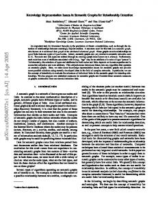
5.2. Example, Continued Figure 1 shows two sensitivity plots for our running example of camera translation. The scenario is exactly the same in both figures: a relatively tight cloud of ten points is placed at about five focal lengths away from the camera, and about two focal lengths off the optical axis to the right, in the direction of the camera’s x axis. The camera translates by one focal length in varying directions. The circle on the ground plane of the plots in figure 1 represents the hemisphere of forward-moving camera translations. For each
Fig. 1. Sensitivity of the most sensitive component of camera translation as a function of the direction of motion. The maximum value on the rim of both plots is : of the amount of translation (translation amount is one focal length) . Image noise was set to be i.i.d., Gaussian, and isotropic, with a standard deviation of : of the camera’s focal length.
0 3%
0 1%
The plot on the right of figure 1, for the spherical representation of translation, had to be truncated in the middle, as emphasized by the circular hole in the middle of the contour plot. This is because the spherical representation has a singularity along the optical axis (forward motion), where the declination angle � is zero, and the azimuth � is therefore undefined. At the singularity, sensitivity goes to infinity. However, there is nothing particularly bad about forward motion. In fact, as the fair plot on the left of figure 1 shows, forward motion is close to optimal, as the minimum sensitivity is reached for a motion approximately toward the point cloud. The problem with the plot on the right is that spherical coordinates are an unfair representation of translation: sensitivity is in the representation, not in the problem itself. Although both plots are correct, the one on the right is misleading, because it mixes the intrinsic sensitivity of the estimation problem with the sensitivity caused by a poor parametrization. Notice that also the minimum moves to a different position between the two plots, as a result of the unfair representation on the right. If the underlying reference frame is changed by a rigid transformation, the plot on the left will be merely shifted. The plot on the right will change in more complex ways,
0-7695-0164-8/99 $10.00 (c) 1999 IEEE
essentially superimposing the fixed singularity of the representation with the changing distribution of sensitivity peaks and valleys that are inherent to the problem. The plot on the left speaks about the sensitivity of the problem; the one on the right conveys a mixed message. Of course, a singularity is a particularly dramatic example of unfairness, because it introduces infinite sensitivities. However, any amount of unfairness will lead to misleading plots that are hard to interpret and can lead to false conclusions.
The form of equation (3) emphasizes the relationship between ideal measurements y� and unknowns #. However, various other parameters appear in most estimation problems. For instance, in the camera translation example, different sensitivity measures result from different distributions of the feature points in space. It would therefore seem that the validity of any sensitivity analysis of the problem is limited to the particular constellation of points under study. Fortunately, this is not so. For every value of camera translation t, point constellations can be grouped into equivalence classes, such that two constellations lead to exactly the same sensitivity. Intuitively, this is because the position of the points affects sensitivity only through the � matrix ^ t as computed through equation (14). In this section, we first show how each of the points in a given constellation can be moved without altering the sensitivity of the translation estimate to image noise. This is a weak result, but intuitively appealing. Then, we give a stronger characterization of equivalence classes, by showing that each class has a representative with just two world points. This allows much more concise and meaningful reports of sensitivity results for problems with many parameters. In the appendix we prove the following preliminary result.
3 3
�
�
T
�,1
Jt =
N X p=1
�
�
^
Theorem 7 Given any camera translation t and any cloud of points in the world, let
�t = � v + � v ^
ep eTp
,
�
z 2 + (z 0 )2 sin2 � p
p
p
We can therefore conclude as follows. Theorem 6 If image noise is Gaussian, small, zero-mean, i.i.d., and isotropic, then the covariance ^t of the ML estimate t of camera translation does not change if the points in the world are moved within their epipolar planes and without changing their depths.
�
1
1
2
(17)
2
�
be the SVD of the rank-2 covariance matrix ^t . Then any two world points on the epipolar planes with normals
e1 = v1
e2 = v 2
and
and at depths p
where ep is the unit vector orthogonal to the epipolar plane of up , and �p is the angle between ep and the optical axis.
^
�
z =
Lemma 1
Jt Jy Jy
�,1
�
T it follows that the product JtT Jy Jy Jt then remains constant, and so does ^t , because of corollary 1, and because under the hypotheses of the theorem the covariance � of image noise is proportional to the identity matrix. Given a particular motion t and an image point up , define the equivalence line of that point to be the intersection of its epipolar plane with the constant-depth plane Z zp through the world point. Then, point clouds that differ only by moving any of their points along their equivalence lines produce the same sensitivity in the translation estimate t. These point clouds therefore belong to the same sensitivity equivalence class. This result implies in particular that the field of view is a poor predictor of the quality of camera translation estimates, because it can be changed at will, without affecting sensitivity, by moving the world points along their equivalence lines. However, two point clouds that differ other than by shifts along equivalence lines can still yield the same sensitivity. The following result gives a stronger characterization of equivalence classes:
=
6. Equivalent Scenarios
T
To prove this, consider a fixed value of translation t. If the world points are moved as stated in the theorem, neither ep (and therefore �p) nor zp , zp0 change. From the lemma,
r
�
p
(1 + t ) sin � 2 3
2
, p
p = 1; 2 :
(recall that t3 is the third component of t, and �p was defined in lemma 1) yield a camera translation estimation problem with exactly the same covariance ^t .
�
�
Proof. We saw in the proof of corollary 1 that ^t has rank 2. From the same corollary, and equation (17), we know that �
Jt Jy �� Jy T
T
�,1
Jt = �1 v1 + �1 v2 : 1
2
By comparing this equation with the expression in Lemma 1, and noting that zp2 zp0 2 zp2 t23 , we obtain the desired result.
0-7695-0164-8/99 $10.00 (c) 1999 IEEE
+ ( ) = (1 + )
�
7. Conclusion In this paper, we have developed general tools for the sensitivity analysis of ML estimation problems. The implicit formulation with constraints lends itself well to the type of problems that arise in various computer vision problems, and we have used the simple problem of estimating camera translation as an illustration. Our generalization of the Gauss-Markov theorem allows analyzing the sensitivity of these problems to small perturbations of the image measurements, and our notion of a fair parametrization leads to sensitivity figures that are independent of the reference system chosen for the analysis. Our results on equivalence classes for sensitivity greatly simplify the task of reporting sensitivity figures for a large family of scenarios. The proposed techniques are general, and are likely to be applicable to more complex problems than camera translation. Acknowledgment: This work was supported by the Deutsche Forschungsgemeinschaft (DFG), grant Ho 1791/21, and by ARO-MURI grant DAAH04-96-1-0007. We thank the anonymous reviewers for several useful comments.
[13] H. C. Longuet-Higgins. A computer algorithm for reconstructing a scene from two projections. Nature, 293:133– 135, September 1981. [14] J. Oliensis. A multi-frame structure-from-motion algorithm under perspective projection. Technical report, NEC, Princeton, NJ, 1998. [15] J. Weng, N. Ahuja, and T. S. Huang. Optimal motion and structure estimation. IEEE Transactions on Pattern Analysis and Machine Intelligence, 15(9):864–884, September 1993. [16] J. Weng, T. S. Huang, and N. Ahuja. Motion and structure from two perspective views: Algorithms, error analysis, and error estimation. IEEE Transactions on Pattern Analysis and Machine Intelligence, 11(5):451–476, May 1989. [17] Z. Zhang. Determining the epipolar geometry and its uncertainty: a review. International Journal of Computer Vision, 27(2):161–195, 1998.
A. Proof of Lemma 1 From the expressions for Jt and Jy derived in sections 3 and 4, we easily obtain �
Jt Jy Jy T
References [1] W. M. Boothby. An Introduction to Differentiable Manifolds and Riemannian Geometry. Academic Press, New York, NY, 1975. [2] J. J. Craig. Introduction to Robotics — Mechanics and Control. Addison-Wesley Pub. Co., Reading, MA, 2nd edition, 1989. [3] A. G. (Editor). Applied Optimal Estimation. The MIT Press, Cambridge, MA, 1974. [4] O. Faugeras. Three-Dimensional Computer Vision — A Geometric Viewpoint. MIT Press, Cambridge, MA, 1993. [5] W. F¨orstner. Reliability analysis of parameter estimation in linear models with applications to mensuration problems in computer vision. Computer Vision, Graphics and Image Processing (CVGIP), 40(1):273–310, October 1987. [6] G. H. Golub and C. Reinsch. Singular Value Decomposition and Least Squares Solutions, volume 2, chapter I/10, pages 134–151. Springer Verlag, New York, NY, 1971. [7] G. H. Golub and C. F. Van Loan. Matrix Computations. The Johns Hopkins University Press, Baltimore, MD, 1996. 3rd edition. [8] J. D. Gorman and A. O. Hero. Lower bounds for parametric estimation with constraints. IEEE Transactions of Information Theory, 36(6):1285–1301, November 1990. [9] B. K. P. Horn and E. J. Weldon Jr. Direct methods for recovering motion. International Journal of Computer Vision, 2:51–76, 1988. [10] K. Kanatani. Geometric Computation for Machine Vision. Clarendon Press, Oxford, England, 1993. [11] K. Kanatani. Statistical optimization for geometric computation : theory and practice. Elsevier, Amsterdam, 1996. [12] J. J. Koenderink and A. J. van Doorn. Facts on optic flow. Biological Cybernetics, 56(4):247–255, 1987.
T
�,1
,
�,
�T
up � u0p up � u0p , � Jt = k (up � t)1;2 k2 + k u0p � t 1;2 k2 p=1 N X
12
where the subscript ; denotes the first and second component of a vector. We can eliminate u0p by equation (6). Since a � a for any vector a, we obtain
=0
�
Jt Jy Jy T
T
�,1
Jt =
N X p=1
(u � t) (u, � t) � k (u � t) k z + (z 0 ) T
p
p
p
1;2
2
2
p
p
2
and
up � t k (up � t)1;2 k
= kuu �� ttk k (uku ��t)tk k = sine � ; so we can conclude as promised. �
0-7695-0164-8/99 $10.00 (c) 1999 IEEE
p
p
p
p
p
1;2
p