Landscape and Urban Planning 150 (2016) 36–49
Contents lists available at ScienceDirect
Landscape and Urban Planning journal homepage: www.elsevier.com/locate/landurbplan
Representing composition, spatial structure and management intensity of European agricultural landscapes: A new typology Emma H. van der Zanden a,∗ , Christian Levers b , Peter H. Verburg a , Tobias Kuemmerle b,c a
Environmental Geography group, Department of Earth Sciences, VU University Amsterdam, De Boelelaan 1085, 1081 HV Amsterdam, The Netherlands Geography Department, Humboldt-University Berlin, Unter den Linden 6, 10099 Berlin, Germany Integrative Research Institute on Transformations in Human-Environment Systems (IRI THESys), Humboldt-University Berlin, Unter den Linden 6, 10099 Berlin, Germany b c
h i g h l i g h t s • • • • •
We present a spatially-explicit typology of European agricultural landscapes. Datasets representing land cover, landscape structure and land management are used. An expert-based top-down typology is compared with a data-driven bottom-up approach. Inclusion of land management differentiates our results from existing typologies. We find clear overlaps in general landscape patterns with existing typologies.
a r t i c l e
i n f o
Article history: Received 18 November 2014 Received in revised form 26 January 2016 Accepted 4 February 2016 Keywords: Agricultural landscapes Landscape typology Land use intensity Self-organizing maps Europe Land management
a b s t r a c t Comprehensive maps that characterize the variation in agricultural landscapes across Europe are lacking. In this paper we present a new Europe-wide, spatially-explicit typology and inventory of the diversity in composition, spatial structure and management intensity of European agricultural landscapes. Agricultural landscape types were characterized at a 1 km2 resolution based on Europe-wide datasets that represent land cover, landscape structure and land management intensity. Two alternative approaches for typology development were used: an expert-based top-down approach, and a bottom-up approach based on automated clustering using Self Organizing Maps (SOMs). Comparison with available national and European landscape typologies showed that our typology deviates from existing biophysical and anthropocentric typologies relevant to agricultural landscapes as result of the inclusion of land management aspects. Concordance occurred between specific European typology classes, while the comparison with national landscape typologies showed a correspondence in agricultural landscape patterns. Our agricultural landscape typology can provide a basis for landscape assessment at a European-scale to help to identify agricultural landscape types prone to change and landscapes that may require policy response. © 2016 Elsevier B.V. All rights reserved.
1. Introduction Land use has transformed more than 80% of the global land surface, by conversion of natural ecosystems into agriculture or cities or by using natural ecosystems at varying intensity (Ellis, Klein Goldewijk, Siebert, Lightman, & Ramankutty, 2010). While much research has focused on how land conversions create agricultural and other human-dominated landscapes (Ramankutty et al., 2006;
∗ Corresponding author. E-mail addresses:
[email protected] (E.H. van der Zanden),
[email protected] (C. Levers),
[email protected] (P.H. Verburg),
[email protected] (T. Kuemmerle). http://dx.doi.org/10.1016/j.landurbplan.2016.02.005 0169-2046/© 2016 Elsevier B.V. All rights reserved.
Verburg, van Asselen, van der Zanden, & Stehfest, 2013), much less attention has been paid to characterizing the spatial variation in agricultural landscapes that has developed in relation to the variation in management intensity within these landscapes, even though management intensity is a main driver of rural landscape change in many world regions (Sayer et al., 2013). Three important dimensions of present-day agricultural landscapes are land cover, land management and landscape structure (Verburg et al., 2013). Land cover types and their arrangement determine the overall agricultural type. Land management refers to the “ways in which humans treat vegetation, soil, and water” for a specific purpose (Lambin, Geist, & Rindfuss, 2006); in other words, the land use practices that people carry out within broad
E.H. van der Zanden et al. / Landscape and Urban Planning 150 (2016) 36–49
land cover types. Examples of such practices include use of fertilizers or pesticides, irrigation schemes and tillage (e.g., Erb et al., 2013; Follett, 2001). Land management can impact landscape functioning and ecosystem services supply substantially (Tscharntke, Klein, Kruess, Steffan-Dewenter, & Thies, 2005; Zhang, Ricketts, Kremen, Carney, & Swinton, 2007). While such effects have been extensively studied at the local scale (e.g., Shriar 2000; Herzog et al., 2006), the spatial patterns of land management at regional to global scales, and thus their impacts on ecosystem functioning, services and biodiversity, are often ignored (Kuemmerle et al., 2013; Verburg et al., 2013). Landscape structure is scale-dependent and refers to the spatial heterogeneity of the landscape (Turner, 1989), for example the arrangement of land uses or cropland fields, or the prevalence of linear landscape elements (e.g., hedges, ditches, terraces, Paracchini et al., 2012; Kumaraswamy & Kunte, 2013). On a regional scale, landscape structure is closely linked to ecosystem services provisioning, especially for a number of regulating services (e.g. erosion prevention, pollination) and cultural services (e.g. landscape aesthetics and tourism, Pinto-Correia & Breman, 2008; Power, 2010; Syrbe & Walz, 2012; van Zanten et al., 2013), as well as the biodiversity-friendliness of agricultural landscapes (Burel & Baudry, 1995; Dramstad et al., 2001). Land cover, land management, and landscape structure are also central features differentiating landscapes with exceptional cultural heritage and values (Plieninger, Höchtl, & Spek, 2006). Cultural landscapes – a term adopted in the 1990s by international bodies as a conservation category (Jones, 2003) – often have relatively high structural complexity, traditional, low-intensity landscape practices and historical elements, altogether contributing to the often exceptional value of these landscapes (Antrop, 2005; Fischer, Hartel, & Kuemmerle, 2012; Plieninger & Bieling, 2012). Many cultural landscapes, however, have recently undergone stark transformations as new land-use paradigms based on more intensive agricultural production are adopted (Vos & Meekes, 1999). Europe is particularly rich in landscapes that are recognized for their natural and cultural heritage (Vos & Meekes, 1999; Plieninger, Höchtl, & Spek, 2006). Many of these cultural landscapes have been shaped by traditional land uses and contain high conservation values that are dependent on continuation of low-intensity agricultural practices (Dieterich & van der Straaten, 2004; Fischer et al., 2012). Historical socioeconomic and institutional events shaped landscape structure and are visible in the landscape today. An example is the high level of fragmentation of ownership and field sizes in post-socialist countries, which is a result of collectivization of land during the socialist time and the re-privatization processes since 1989 (Hartvigsen, 2014; Kuemmerle et al., 2008). Conserving European cultural landscapes, as well as their cultural and natural heritage has received increased attention in European policy making recently, with the introduction of the High Nature Value (HNV) farmland concept as the clearest example (EEA, 2010; Kleijn, Rundlöf, Scheper, Smith, & Tscharntke, 2011; Paracchini et al., 2008; Robinson & Sutherland, 2002; Walz & Syrbe, 2013). Furthermore, specific EU policies, such as the Common Agricultural Policy (CAP), increasingly promote a landscape-based approach (Paracchini & Capitani, 2011), although there is also critique on the dominant environmental focus of landscape management in these policies (Agnoletti, 2014). To better understand the large spatial heterogeneity of agricultural landscapes across Europe, and to monitor changes in landscape functions and values, it is necessary to reduce the complexity in agricultural landscapes to manageable units that could be an interesting target for policy-making at the European scale. Several initiatives have sought to identify and classify landscapes in Europe since the 1990s (Paleo, 2010), including the PanEuropean Biological and Landscape Diversity Strategy (PEBLDS, Council of Europe 1996) and the European Landscape Conven-
37
tion (ELC, Council of Europe 2000). The ELC encouraged member states to identify and assess the national landscapes and their features, but with a focus on member state autonomy and a clear subsidiarity principle (Council of Europe, 2000). Thus, the national landscape maps differ substantially in mapping approaches (see Supplementary material A), data sources, and the underlying landscape-concept (i.e., interpretation of the role of humans in the landscape; see Angelstam et al., 2013 for an overview; Cassatella & Voghera, 2011; Groom, 2005). Substantial progress in developing a Pan-European Landscape map, an important action theme of the PEBLDS (Council of Europe, 1996), was made. Meeus (1995) developed a qualitative classification of traditional European landscapes. Building on this, Mücher et al. (2010) developed a Landscape Map (LANMAP) aimed to give an overall classification of landscape types in Europe, based on quantitative spatial analysis and a consistent classification framework. However, previous research efforts have not incorporated key dimensions that are important for differentiating agricultural landscapes, such as land management and landscape structure. Our main objective is to focus on this research gap, by developing a typology of the diversity in composition, spatial structure and management intensity of European agricultural landscapes. By focusing on these selected dimensions, we aim to provide a generic basis (i.e., independent from specific locations or geographic contexts) for assessment and comparison of agricultural areas in Europe. Such an approach is highly complementary to existing classifications and typologies which mainly capture biophysical dimensions of landscapes in great detail. A second objective is to compare methods for typology development. As traditional approaches in typology development either take a top-down or a bottom-up approach, we compared an expert-based top-down, and a bottom-up approach based on automated clustering. Europe is an interesting case for such analysis, as landscape characterization and assessment is a key aspect in European landscape research (Plieninger, Dijks, Oteros-Rozas, & Bieling, 2013). But the typology development also provides a methodological example for the delineation of agricultural typologies for other world regions, moving beyond the standard approach of characterizing differences in landscape and land use by their dominant land cover only (e.g., Busch, 2006; Verburg et al., 2013). The representation of critical aspects of agricultural landscapes is currently lacking on a regional scale, while progress has been made with global scale typologies (see Verburg, van Asselen, van der Zanden, & Stehfest, 2013). Improved representation of agricultural landscapes within subglobal assessments can furthermore clarify landscapes’ influence on environmental change (Verburg, van Asselen, van der Zanden, & Stehfest, 2013).
2. Materials and methods Traditional approaches to develop landscape typologies using geospatial data have applied either a top-down or bottom-up approach. In a top-down approach, the typology is commonly delineated based on a decision tree defined by expert rules and supervised threshold selection (Maxwell & Buddemeier, 2002). A bottom-up approach, in contrast, determines landscape types based on groups of locations that have similar characteristics, usually with the help of statistical clustering methods. We used both of these approaches, specifically a top-down expert-based classification and a bottom-up approach based on automated clustering using self-organizing maps (SOMs) (see Fig. 1), that used the same input data for the land cover, land management and landscape structure dimensions of agricultural landscapes. We then carried out a map comparison to assess the influence of method selection on the resulting maps.
38
E.H. van der Zanden et al. / Landscape and Urban Planning 150 (2016) 36–49
Fig. 1. Methodology of agricultural landscape typology development.
Table 1 Input data for the classification of the diversity in composition, spatial structure and management intensity of European agricultural landscapes. Agricultural landscape dimension
Dataset
Unit
Resolution
Time period
Source
Dominant land use
CORINE Land use/cover
Area (250 m)
1 km2
2006
Land management
Fertilizer application rates
N application class (kg N/ha)
1 km2
2003–2006
CLC 2006 land cover (www.eea. europa.eu/dataand-maps/) Temme & Verburg (2011), Overmars et al. (2014)
Landscape structure Landscape structure
Field size
Size class in ha
1 km2
2009
Linear landscape elements
Number of intersections with elements
1 km2
2009
2.1. Datasets used To represent the land cover, land management and landscape structure dimensions of agricultural landscapes, we used a range of independent datasets which are publicly available for the territory of the European Union (Table 1). Regarding information on land cover, we used the CORINE land cover (CLC) map (EEA, 2005) to select agricultural areas using non-irrigated arable land (CLC 2.1.1), permanent crops (CLC 2.2), pasture (CLC 2.3) and heterogeneous agricultural areas (CLC 2.4). We aggregated this information to 1 km2 raster cells using a majority rule. Regarding information on land management, we used nitrogen input as a proxy for the use of capital-intensive inputs to agriculture. Nitrogen input is often used as an indicator for agricultural intensification due to its strong effects on the biodiversity of agricultural landscapes, although a combination of different indicators may better capture patterns of intensity (Erb et al., 2013; Herzog et al., 2006). We created the nitrogen input map following Temme and Verburg (2011) and Overmars et al. (2014). This approach was chosen because the resulting pixel-based maps were more suitable for our purpose than nitrogen input levels reported in statistics for national or sub-national administrative units. The creation of nitrogen input maps began with nitrogen
Kuemmerle et al. (2013) van der Zanden et al. (2013)
Validation
The intensity classes are tested by reviewing the data assignment to irrigated vs. non-irrigated areas (CORINE 2000). In Supplementary Material B. Independent validation of green lines based on aerial photographs (van der Zanden et al., 2013)
input levels (kg/ha) at sub-administrative level (NUTS 2) per crop type per administrative unit, available from the Common Agricultural Policy Regionalized Impact modelling System (CAPRI; Britz, 2005; Leip et al., 2008). These nitrogen input levels were downscaled to the pixel level using point-based crop observations in the same administrative units assuming that the cropping pattern can serve as a proxy for the variation in nitrogen application within an administrative unit. We used point-based observations from the 2003 and 2006 land use/cover area frame statistical surveys (LUCAS) database (∼150.000 sample points, Delincé 2001; Gallego & Delincé 2010). The LUCAS project, which currently has five sampling years (2001, 2003, 2006, 2009 and 2012), collects field observations and includes information on land cover/use and additional visual information, e.g., on slope, field size, water management and grazing (Eurostat, 2009). In recent survey years, the number of sample points was extended and the sampling scheme was adjusted (Gallego & Delincé, 2010). The possible influence of different sampling schemes on the nitrogen input was evaluated by Temme & Verburg (2011) which showed that the higher spatial autocorrelation in the 2003 LUCAS dataset does not strongly affect the results of the method. In our approach, we reclassified the CAPRI based nitrogen application rates assigned to each LUCAS point into three classes: low intensity (150 kg N/ha), based on the variation of nitrogen application rates throughout Europe (see Leip et al., 2008) and the relevance of these levels for biodiversity in agricultural areas (Kleijn et al., 2009). With respect to agro-biodiversity, a threshold of 150 kg N/ha). After the reclassification of the nitrogen input levels the point observations were extrapolated to all cropland pixels using country-specific multinomial regression models and a set of environmental and socio-economic location factors. Grassland was modeled using a different approach, where we estimated nitrogen input based on local cattle stocking densities using livestock maps from Neumann et al. (2009) and assuming a uniform quantity of 100 kg N/ha per cow per year (van Grinsven et al., 2015; van der Hoek, 1998), based on total N of dairy cattle minus the N in animal products (e.g., milk). Following the approach of Temme & Verburg (2011), nitrogen input was reclassified into two classes; extensive (50 kg N/ha) grasslands. As indicators for landscape structure, we used field size and the density of green linear landscape elements. Field size captures the spatial configuration of fields as well as important components of land management history, as current field size is often influenced by field patterns of the past (e.g., Sklenicka et al., 2009). Also, in other studies field size is used as a variable to characterize the agricultural landscape structure (Geiger et al., 2010). We based the field size information on the 2009 LUCAS database which provides field size information at the sampling point based on observers estimating the size of the agricultural parcel belonging to one out of the following classes: 1) less than 0.5 ha, 2) greater than or equal to 0.5 ha and less than 1 ha, 3) greater than or equal to 1 ha and less than 10 ha, 4) greater than 10 ha (Eurostat, 2009). We interpolated the field size class information to a 1 km2 raster with European coverage using an Ordinary Kriging method (K-means variogram model with 50 observation points in the search radius), which gave the best results in a comparison of different kriging methods. Comparable field size classes and method are used for mapping field size on a global scale by Fritz et al. (2015). We validated the field size information using 150 randomly generated 10 km by 10 km sampling squares in agricultural and mosaic landscapes. In these sampling squares, the field size was analyzed for 5 random points according to the LUCAS sampling procedures using high-resolution images from Google Earth. For further details on the validation see Supplementary material B. Linear landscape elements provide important interconnections in heterogeneous landscapes and are explicitly acknowledged as important cultural features, and linked to recreational, aesthetical, and heritage values (Burel & Baudry, 1995). Green linear landscape elements also provide important ecological functions, such as ecological corridors, pollution control, pollination, and erosion and wind control (see overview in van der Zanden, Verburg, & Mücher, 2013). Other landscape elements such as agricultural ditches, terraces or grass margins are also potentially important (Herzon & Helenius, 2008; Oslon & Wäckers, 2007), but not included here due to data limitations. We used a map of linear landscape elements described in detail in van der Zanden et al. (2013). As a basis for this map, the transect information on linear elements from the 2009 LUCAS database was used. On each 250 m transect, surveyor’s report crossings of linear landscape features (features wider than 1 m and at least 20 m long, except for walls and fences). This information was collected for 19 classes of linear landscape elements, of which a combination of avenue trees, conifer and bush/trees hedges (managed and non-managed), grove/woodland margins, heath/scrub and dry stone walls were selected. van der Zanden et al.
39
(2013) interpolated the point count information per transect to the 1 km2 pixel level using Zero-Inflated Negative Binomial (ZINB; Lambert, 1992) regression models, with different biophysical and socio-economic location factor data as independent variables. Several case studies highlight linkages between agricultural intensity and landscape structure, although such broad generalizations can be misleading (Roschewitz, Thies, & Tscharntke, 2005). For example, Rodríguez and Wiegand (2009) investigated machineefficiency originating field enlargement in Southern Spain, as agricultural intensification and scale-enlargement often leads to an increased field size. Thenail (2002) and Thenail and Baudry (2004) analyzed the influence of a gradient of decreasing hedgerow density and increasing field size, showing that a decrease in hedgerow density was related to increased production and technical means in dairy farms. Land-use allocation in farms was also dependent on hedgerow density, thereby influencing the landscape structure.
2.2. Expert-based typology Landscape typologies are often based on a combination of expert-based rules and numerical analysis. A notable example of this approach is Meeus (1995), who developed the first approach towards a European landscape map by qualitatively combining information from national typologies, maps and scientific expertise. In several national typologies this method was also used, ranging from pure expert-based interpretation (e.g., Hungary; Márton, 1989) to the combination of thematic maps to form a composite map (e.g., Lithuania; Kavaliauskas & Veteikis, 2006). In general, expert-based landscape typologies can be described as topdown, hierarchical delineations in which the subdivision of an area is based on a synoptic view and usually executed by expert rules and supervised threshold selection. Such classifications are typically based on a limited number of variables to keep the interpretation of classification trees manageable (Maxwell & Buddemeier, 2002; Van Eetvelde & Antrop, 2009). For the division of the land cover categories, we relied on the CORINE land cover classes: arable land, grassland, permanent crops and mosaic land cover. We reclassified the linear landscape elements map (van der Zanden et al., 2013) into two classes: presence and non-presence, to distinguish open and more enclosed landscapes. We chose the threshold for this division based on the correspondence with presence of known areas of enclosed landscapes within European typologies (bocage and semi-bocage) and documentation of the characteristics of these landscapes (e.g., Zimmermann, 2006 and the digitized version of the Meeus landscape map in Stanners & Bourdeau 1995). We aggregated the field size classes into three classes: small-scale (10 ha), based on presence of these classes in the study area. For the nitrogen input, we used the classes of the original dataset. To delineate the landscape classes we developed an expertbased decision tree in order to follow a systematic classification of landscape types (Fig. 2). To prevent delineation of too many classes, we combined classes that overlapped in character into meaningful aggregates based on secondary information such as country reports, national typologies and informal consultation with landscape experts. Furthermore, if classes were negligible in area for the European Union (10 km2 are displayed.
in Austria and Poland. For grassland, there was no clear regional divide between the more extensive and intensive areas. Enclosed grasslands occurred in large continuous areas; geographically limited to the Western UK and Ireland, Northern Germany, Northern Netherlands and North-West and Central France. The enclosed mosaic landscapes were generally linked to the enclosed grassland areas, with the exception of Galicia (North-West Spain) which was characterized by a mixture of extensive and intensive enclosed mosaic lands. The open mosaic landscapes occurred in different areas that were sometimes characterized by viniculture.
3.2. SOM results The number of SOM clusters was determined by analyzing the natural breakpoints in a number of performance indicators upon
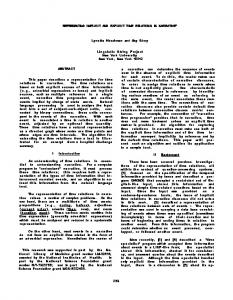
an increase in number of clusters. Fig. 5 shows the mean and standard deviation of the distance of values to the codebook vector and the Davies–Bouldin Index value. The clustering indices showed a natural breaking point at 12 clusters. A further comparison of the resulting classifications of the 3 × 4 and 4 × 5 SOM grids confirmed that 12 clusters capture the main variation between the landscapes well. A SOM plot gives information on the specific relationship between the input data and the SOMs (Fig. 6). The spatial location of the cluster in the segment plot indicates the similarity with the other clusters while the segments indicate the contribution of the different variables in determining the cluster. The segment plot indicates two general groups of agricultural landscapes: 1) arable landscapes that mainly vary in land management (top-right) and
42
E.H. van der Zanden et al. / Landscape and Urban Planning 150 (2016) 36–49
Fig. 4. Detailed legend for the agricultural landscapes as delineated by the expert-based typology.
2) mosaic and grassland landscapes defined by landscape structure (bottom-row).
The agricultural landscapes as delineated by the SOM typology are shown in Fig. 7. An interpretation describing the different clusters and the average values of the non-standardized values of the
E.H. van der Zanden et al. / Landscape and Urban Planning 150 (2016) 36–49
43
Fig. 5. Mean and standard deviation of the distance of values to the codebook vector and the Davies–Bouldin Index value for an increasing number of clusters.
Fig. 6. Segment plot of 3 × 4 SOM clusters with their cluster number and the distance of each cluster to the winning unit.
different input datasets are available in Supplementary material E and F. Fig. 8 shows the map of the distance of each raster cell to the codebook vector, which can be regarded as a quality assessment of the classification procedure. Regions with a large distance to the winning SOM unit are Southern Spain, Northern Ireland and Brittany (North-West France). This indicates that in these regions, the assigned SOMs are not optimal to capture the variability in occurring agricultural landscapes.
In general, the differences are caused by the aggregation of the more specific expert-based categories in single classes in the SOM classification. For example, cluster 3 in the SOM (“enclosed grassland”) includes both small-scale and enclosed grassland classes of varying intensity and scale. SOM cluster 12 (“large-scale arable land”) includes large-scale arable classes from all intensities of the expert based typology. Some classes that are, from an expert perspective, important to distinguish are not sufficiently differentiated in the spatial data to appear as separate classes in the SOM typology.
3.3. Comparison between mapping approaches Spatial comparison between the two different approaches used to construct the typology shows that there is, in general, a large overlap between classes. Such overlap between both methodologies is not surprising as both the expert-based and SOM method aim at classification of the diversity of the composition, spatial structure and management intensity of agricultural landscapes. An exact overlap exists between three SOM classes (cluster 8, 9 and 11) and expert-based classes (large-scale extensive arable land, mediumscale intensive arable land and large-scale very intensive arable land respectively), while cluster 10 is a combination of the smallscale and large-scale permanent crops classes. A cross-tabulation between the mapping approaches is available in Table 2.
3.4. Comparison with other typologies and national landscape classifications To assess the relationship between our typology and widely used European datasets, we selected maps that capture different aspects of the agricultural landscape, including climate and biophysical dimensions. We included the climate-focused Environmental Stratification of Europe (EnS) and the LANMAP classification, which has four separate levels (Mücher et al., 2010). We also used the European Environment Agency (EEA) landscape types map, which is based on a neighborhood analysis of land cover types (EEA, 2006), the analogue Meeus landscape map as digitized in Stanners and Bourdeau (1995) and the Anthromes map (Ellis &
44
E.H. van der Zanden et al. / Landscape and Urban Planning 150 (2016) 36–49
Fig. 7. Agricultural landscapes as delineated by the SOM based typology. A detailed legend is available in Supplementary material E.
Ramankutty, 2008), which is based on global data on population, land use and land cover. The highest agreement exists between the SOM and the expertbased map (75.5%) developed in this study. These maps are not independent, due to the similar input data and similar aims. The results in Table 3 clearly show that our typologies capture very different dimensions of the agricultural landscape as compared to the other datasets, as the concordance with the other included datasets is low to very low (Hargrove et al., 2006). More specifically, the expert-based typology shows the highest concordance with the climate dimension of LANMAP (level 1), followed by the EEA land cover based map and the EnS climatic zones. These agreements were likely the result of the partial overlap of the “broad pattern intensive agriculture” of the EEA land cover based map with the medium intensive arable and very intensive arable land classes and by the overlap between the continental climate zone with very intensive arable areas. The SOM map also has a high agreement with the LANMAP level 1 and EEA dominant landscapes, followed
by the Meeus map. This mainly is based on the enclosed grassland cluster, which has a high agreement with both “rural mosaic and pasture landscapes” (EEA) and “Atlantic Bocage” as delineated in the Meeus map. Another European map useful for a comparison is the Types of Agriculture Map of Europe (Kostrowicki, 1984). While the map is outdated, the classification used compares well with our present work, as it accounts for the scale and intensity dimensions by using land use statistics, input-related statistics, production attributes and structural attributes (permanent crops, permanent grassland, and livestock). It was not possible to quantitatively compare this map as no digital version is available. A visual comparison with our typologies showed clear differences for the regions that faced widespread scale enlargement and intensification in the past 30 years, such as in Southern Denmark and the agricultural region around Paris (France). But we also found remarkable similarities, for example, between French regions with small-scale intensive
E.H. van der Zanden et al. / Landscape and Urban Planning 150 (2016) 36–49
45
Fig. 8. Distances of raster cells to the codebook vector of the 3 × 4 SOM clusters. Low values indicate a good quality of mapping. Table 2 Cross-tabulation between the expert-based and the SOM-based typology (in km2 ). Expert-based classes
1 2 3 4 5 6 7 8 9 10 11 12 13 14 15 16 17 18 19
SOM-based classes 1
2
3
4
5
6
7
8
9
10
11
12
0 0 0 0 0 0 0 0 0 0 0 0 50032 0 57888 0 16998 0 0
0 0 0 0 0 0 0 0 50640 9596 0 76235 0 0 0 0 0 0 0
0 0 0 0 0 0 0 13107 0 5155 71591 0 0 0 0 0 0 0 0
0 0 0 0 0 0 0 0 0 0 0 0 10180 0 13087 0 3578 0 0
0 0 0 0 0 0 0 0 0 0 0 0 0 14798 0 26407 6210 0 0
941 4521 1567 13608 820 1431 7980 0 0 0 0 0 0 0 0 0 0 0 0
17565 0 26836 0 0 15909 0 0 0 0 0 0 0 0 0 0 0 0 0
0 0 0 289765 0 0 0 0 0 0 0 0 0 0 0 0 0 0 0
0 0 0 0 0 0 171804 0 0 0 0 0 0 0 0 0 0 0 0
0 0 0 0 0 0 0 0 0 0 0 0 0 0 0 0 0 16589 53403
0 172620 0 0 0 0 0 0 0 0 0 0 0 0 0 0 0 0 0
0 17587 0 0 24662 0 13669 0 0 0 0 0 0 0 0 0 0 0 0
grassland (e.g., Normandy and S-Auvergne region) and small-scale mixed agriculture (e.g., Brittany). A qualitative comparison of national landscape classifications shows that the classifications based on land cover display a similar general pattern with our European typologies, for instance in
Austria (Schmitzberger, Szerencsits, & Wrbka, 2001) and the Czech Republic (Hrnciarová, 2009). A closer look at the German typology gives information on land cover and landscape structure dimensions (Gharadjedaghi et al., 2004). Major areas with hedgerows overlap with “enclosed grassland” areas, for instance along the
46
E.H. van der Zanden et al. / Landscape and Urban Planning 150 (2016) 36–49
Table 3 Goodness-of-fit scores using MapCurves (Hargrove et al., 2006).
Expert-based SOM Meeus Anthromes EnS EEA 10 LANMAP level 1 LANMAP level 2 LANMAP level 3 a b c d e
SOM
Meeusa
Anthromesb
EnSc
EEAd
LANMAP l1e
LANMAP l2e
LANMAP l3e
LANMAP l4e
75.5
8.1 12.9
5.1 8.6 4.9
10.2 10.5 17.7 11.3
16.5 16.6 13.9 11.9 12.4
17.9 17.1 30.7 16.0 26.0 14.5
6.3 10.3 11.7 5.2 15.1 12.4 99.9
6.5 10.6 11.0 4.7 15.5 12.5 99.9 100.0
6.9 11.2 13.2 5.4 17.8 13.0 99.9 100.0 100.0
Meeus (1995) as digitized in Stanners and Bourdeau (1995). Ellis & Ramankutty (2008). Metzger et al. (2005). EEA (2006). Mücher et al. (2010) with four levels: climate (1), altitude (2), parent material (3) and land cover (4).
western coastline of the North Sea, the Rhine border region with the Netherlands and around Göttingen (Central Germany). Our typology, however, underrepresents the hedgerow complexes of Baden-Württemberg (South-West Germany; Kantelhardt, Osinski, & Heissenhuber, 2003). While the “structural cultural landscapes” in Bavaria (Southern Germany) clearly overlap with both open and enclosed mosaic landscape classes, this is also not well reflected westwards (Bundesamt für Naturschutz, 2011; Gharadjedaghi et al., 2004). 4. Discussion The shortcomings of landscape information on EU level (Vervloet & Spek, 2003; Wascher, 2004) hamper the comparison of agricultural landscapes across wider geographic scales. While agricultural typologies exist on the national and global scale (Václavík, Lautenbach, Kuemmerle, & Seppelt, 2013 ; van Asselen & Verburg, 2012), there is a need for a better description and representation of the variation in agricultural landscapes at the regional scale. Regional and EU-level policies on conservation and agriculture need to be adapted to the variation in local and regional context (Turner II, Lambin, & Reenberg, 2007; Verburg et al., 2013). Landscape typologies can provide insight and a reduction of the complexity of the variation in agricultural landscapes and thus help to inform and assess the regional needs and consequences. 4.1. Evaluation of methods The evaluation of the quality and robustness of landscape typologies is challenging. To identify the most important components of the landscape represented in the typology, the selection process of the dimensions included should be clear and the scientific theory behind the conceptual framework should be communicated. Since most environmental datasets are continuous, the boundaries between the classes should be reproducible and without personal bias (Hazeu et al., 2011). This is, however, not easy to achieve given the continuous nature of environmental information (Metzger, Bunce, Jongman, & Mücher, 2005). We used two different techniques to develop a landscape typology and in spite of the stark methodological differences (top-down vs. bottom-up) the outcomes show a high degree of agreement. The expert-based approach has the advantage that the construction of the typology is transparent and that the emerging classes are clearly interpretable. However, as in all expert-based typologies, personal judgment cannot be completely excluded (Jongman et al., 2006). The use of the SOM avoids some of these subjective decisions, since this method does not need a supervised classification set-up and instead searches for major structures and clusters without an a priori hypothesis (Agarwal and Skupin, 2008). Moreover, automated
clustering methods can discover unknown patterns in the data, which an expert-based approach rules out. However, while SOM classes display the statistical optimal solution given the current information (and input data), transferring this typology to another dataset, e.g., representing future conditions, is challenging. Therefore, we recommend users to use the expert-based typology for future work. Our typology compared favorably with many national-scale typologies and an outdated land management-based typology (Kostrowicki, 1984), indicating a correspondence of identified types with commonly denoted differences between agricultural landscapes. The typology was robust between the two approaches used, and adds useful dimensions of land management and landscape structure to existing typologies. At the same time, several points of uncertainty need to be discussed. The choice of included dimensions within the developed typology was constrained by data availability and quality on landscape properties and could be expanded by including information on historical or cultural landscape dimensions, especially in applications related to cultural heritage. While our typology takes some of these aspects into account by including landscape structure and field size, important information on e.g., historical features such as agricultural buildings and roads and aesthetic landscape features (e.g., Bastian, Walz, & Decker, 2013; Carvalho-Ribeiro et al., 2013) were missing, since this data is often limited to regions or specific for local sites (Van Eetvelde & Antrop, 2009). Furthermore, information on the social perception of agricultural landscapes could provide information on values and meaning embedded in the landscape. For example, Paracchini and Capitani (2011) presented the development towards an rural-agrarian landscape indicator in Europe, including a composite indicator of societal awareness of landscapes at sub-national administrative level (using protected products, rural tourism and protected areas), while van Zanten et al. (2014) made a systematic review of landscape preference studies in Europe. Another limitation of the current approach is the focus on agricultural areas as designated by the CLC data and the use of a majority rule in the aggregation of the land cover data to the 1 km2 resolution. This may have caused certain heterogeneous mixed farming-forestry or semi-natural areas that are extensively grazed to be underrepresented in our map. Finally, since the developed typology focuses on generic agricultural landscape types across Europe, unique regional characters are generalized and this can therefore lead to an underestimation of the regional identity (Mücher et al., 2010). A main factor affecting the quality of the typology is the quality and quantity of the input data. Sources of uncertainty are both related to the processing of the source data as well as to the reliability of ground-based inventories, such as LUCAS (Eurostat, 2013; Kuemmerle et al., 2013; Verburg, Neumann, & Nol, 2011). The European land cover data used has generally high accuracy, although
E.H. van der Zanden et al. / Landscape and Urban Planning 150 (2016) 36–49
identification of specific land cover classes can be problematic (Büttner & Maucha, 2006). Uncertainties in the other datasets are higher. Our own assessment of the uncertainty of the field size data and linear landscape element data (Supplementary material B and van der Zanden et al. (2013)) suggests reliability of these dimensions. Unfortunately, no full uncertainty analysis was conducted for the nitrogen input data due to a lack of validation data at the pixel level. Partial validation based on differences of nitrogen input in irrigated and non-irrigated land use showed, however, promising results (see Temme and Verburg (2011)). A further limitation of the nitrogen dataset is that the intensity measure is not continuous. Other European scale nitrogen datasets have been developed using comparable methods (e.g., Leip et al., 2011 for N flux budgets), but these are not publicly available. Alternative continuous mapping approaches, such as Teillard et al. (2012) are limited to certain countries and in spatial resolution. In general, the different datasets used are not based on data from the same reference year, which could cause some mismatches in regions with rapid change. Since most of the source data is updated every few years, a useful extension of our study would be the identification of typical change patterns in agricultural landscapes.
4.2. Applications Our agricultural landscape typology and map can be used in a wide range of applications. First and foremost, our results may become a tool for communication between scientists, policy makers and others interested in agricultural landscapes. A harmonized approach such as ours can help identify and characterize policy areas of attention, for instance on the linkages between cultural landscapes, landscape structure and biodiversity conservation. This new typology can also serve as a starting point for further analysis, as a first phase of more detailed regional characterization, or as a tool to compare case studies across different agricultural landscapes in Europe. An example is the application of the map to determine the distribution of landscape preference case studies across different agricultural landscape types by van Zanten et al. (2014). Our results can also serve as a basis for sampling, or the (pre-) selection of study sites (Hazeu et al., 2011; Mücher et al., 2010). Our typology can also be a useful tool for the assessment of multiple ecosystem services across agricultural landscapes, since spatial diversity and landscape structure influence service provision. An interesting application of our typology would thus be to use the agricultural landscapes we identified as units to summarize ecosystem bundles (Bennett, Peterson, & Gordon, 2009). Land management and structure are also considered important elements for modeling or comparing individual ecosystem services, such as pollination (Schulp, Lautenbach, & Verburg, 2014) and landscape aesthetics (Gobster, Nassauer, Daniel, & Fry, 2007) and can therefore serve as a basis for mapping these services. Especially since the vast majority of ecosystem services studies use lookup tables and benefit transfer-based mapping based on land cover, ignoring the role of important landscape features and configurations. Also for the mapping of more ‘intangible’ cultural ecosystem services, Plieninger et al. (2013) acknowledge the need for information on landscape properties beyond land cover, for instance for preselection of sites for the assessment of cultural landscape services or to combine with more fine-grained landscape or stakeholder information (Norton, Inwood, Crowe, & Baker, 2012). The typology of agricultural landscapes in Europe presented here explicitly acknowledges the variation within agricultural areas important to the functioning and values of these landscapes and moves beyond the standard approach of characterizing differences in landscape
47
and land use by the dominant land cover only (e.g., Busch, 2006; Verburg et al., 2013). 5. Conclusion The influence of land management intensity and landscape structure on the spatial variation of agricultural landscapes has received little attention in Europe, while these factors are important for assessing landscape functions and values. To improve the understanding of agricultural landscapes across Europe and to identify landscapes that may require policy response, it is necessary to reduce the complexity in agricultural landscapes to manageable units. During the past 20 years, different initiatives have been developed to identify and classify landscapes in Europe, but important management dimensions, including land management intensity and landscape structure, have not been included in these initiatives. To fill this gap, we have developed a Europe-wide spatially-explicit typology and inventory of agricultural landscapes, using Europe-wide datasets representing land cover, land management intensity and landscape structure on a 1 km2 resolution. We have compared two alternative mapping approaches: an expert-based top-down, and a bottom-up approach based on automated clustering using self-organizing maps (SOMs). Despite the clear difference in typology delineation methodology (top-down vs. bottom-up) the outcomes do not differ greatly. Comparison with national-scale typologies, a dated land management typology and other Europe-wide datasets revealed that the developed typology was robust and added useful dimensions to existing typologies. Improvement is possible, for instance by including information on historical and cultural dimensions, which was currently limited by data availability and quality. The quality and quantity of the input data remains influential, e.g., by including non-continuous input data sets. Overall, the typology aimed to provide a generic basis (i.e., independent from specific location or geographic context) for agricultural landscape assessment, complementary to current biophysically focused classifications and typologies. Therefore, it can be seen as a first step towards a comprehensive regional framework for comparison of agricultural landscapes across Europe. Acknowledgements The data are available upon request to the corresponding author. This work was supported by the VOLANTE, HERCULES and CLAIM projects, all funded by the European Commission (FP7 Programme), and the Einstein Foundation Berlin, Germany. The authors would also like to thank the participants of the MSc course Land System Science’ at the Geography Department of Humboldt University Berlin in 2013 for their assistance. Emiel van Loon is thanked for the MapCurves script. Appendix A. Supplementary data Supplementary data associated with this article can be found, in the online version, at http://dx.doi.org/10.1016/j.landurbplan. 2016.02.005. References Agarwal, P., & Skupin, A. (2008). Self-organising maps: applications in geographic information science. New York: John Wiley & Sons, Ltd. Agnoletti, M. (2014). Rural landscape, nature conservation and culture: some notes on research trends and management approaches from a (southern) European perspective. Landscape and Urban Planning, 126, 66–73. http://dx.doi.org/10. 1016/j.landurbplan.2014.02.012 Angelstam, P., Grodzynskyi, M., Andersson, K., Axelsson, R., Elbakidze, M., Khoroshev, A., & Naumov, V. (2013). Measurement, collaborative learning and research for sustainable use of ecosystem services: landscape concepts and
48
E.H. van der Zanden et al. / Landscape and Urban Planning 150 (2016) 36–49
Europe as laboratory. Ambio, 42(2), 129–145. http://dx.doi.org/10.1007/ s13280-012-0368-0 Antrop, M. (2005). Why landscapes of the past are important for the future. Landscape and Urban Planning, 70(1–2), 21–34. Atkinson, P. W., Fuller, R. J., Vickery, J. A., Conway, G. J., Tallowin, J. R. B., Smith, R. E. N., & Brown, V. K. (2005). Influence of agricultural management, sward structure and food resources on grassland field use by birds in lowland England. Journal of Applied Ecology, 42(5), 932–942. http://dx.doi.org/10.1111/j. 1365-2664.2005.01070.x Bastian, O., Walz, U., & Decker, A. (2013). Historical landscape elements: part of our cultural heritage—a methodological study from Saxony. In J. Kozak, K. ˙ Ostapowicz, A. Bytnerowicz, & B. Wyzga (Eds.), The carpathians: integrating nature and society towards sustainability (pp. 441–459). Berlin: Springer, 10.1007/978-3-642-12725-0. Bennett, E. M., Peterson, G. D., & Gordon, L. J. (2009). Understanding relationships among multiple ecosystem services. Ecology Letters, 12(12) http://dx.doi.org/ 10.1111/j. 1461-0248.2009.01387.x, 1394-404 Billeter, R., Liira, J., Bailey, D., Bugter, R., Arens, P., Augenstein, I., & Edwards, P. J. (2008). Indicators for biodiversity in agricultural landscapes: a pan-European study. Journal of Applied Ecology, 45(1), 141–150. Britz, W., 2005. CAPRI modelling system documentation (common agricultural policy regional impact analysis), Institute for Agricultural Policy, Market Research and Economic Sociology, University of Bonn, Bonn. Büttner, G., & Maucha, G., 2006. The thematic accuracy of Corine land cover 2000. Assessment using LUCAS (land use/cover area frame statistical survey). Technical Report. Copenhagen, Denmark. Bundesamt für Naturschutz. http://www.bfn.de/0311 schutzw landsch.html, 2011 Burel, F., Burel, F., & Baudry, J. (1995). Social, aesthetic and ecological aspects of hedgerows in rural landscapes as a framework for greenways. Landscape and Urban Planning, 33(1–3), 327–340. Busch, G. (2006). Future European agricultural landscapes—what can we learn from existing quantitative land use scenario studies? Agriculture, Ecosystems & Environment, 114(1), 121–140. http://dx.doi.org/10.1016/j.agee.2005.11.007 Carvalho-Ribeiro, S., Ramos, I. L., Madeira, L., Barroso, F., Menezes, H., & Pinto Correia, T. (2013). Is land cover an important asset for addressing the subjective landscape dimensions? Land Use Policy, 35, 50–60. http://dx.doi.org/ 10.1016/j.landusepol.2013.04.015 Cassatella, C., & Voghera, A. (2011). Indicators used for landscape. In A. Peano, & C. Cassatella (Eds.), Landscape indicators. assessing and monitoring landscape quality (pp. 31–46). Dordrecht: Springer. http://dx.doi.org/10.1007/978-94007-0366-7 Council of Europe, 1996. The Pan-European Biological and Landscape Diversity Strategy: A Vision for Europe’s Natural Heritage. Strasbourg. Council of Europe. (2000). The European landscape convention. Strasbourg: Council of Europe. Davies, D. L., & Bouldin, D. W. (1979). A cluster separation measure. IEEE Transactions on Pattern Analysis and Machine Intelligence, 2, 224–227. Delincé, J., 2001. A European approach to area frame survey. In Proceedings of the Conference on Agricultural and Environmental Statistical Applications (CAESAR) in Rome, Vol. 2, June 5–7, pp. 463–472. Dieterich, M., & van der Straaten, J. (2004). Cultural landscapes and land use. In The nature conservation—society interface. pp. 219. Dordrecht: Kluwer Academic Publishers. Dramstad, W. E., Fry, G., Fjellstad, W. J., Skar, B., Helliksen, W., Sollund, M. L. B., & Framstad, E. (2001). Integrating landscape-based values. Norwegian monitoring of agricultural landscapes. Landscape and Urban Planning, 57(3–4), 257–268. EEA, 2005. IMAGE2000 and CLC2000. Products and Methods. CORINE Land Cover Updating for the Year 2000. Copenhagen: Ispra, Italy. pp. 1–152. EEA. http://www.eea.europa.eu/data-and-maps/figures/the-dominant-landscapetypes-of-europe, 2006 EEA, 2010. 10 messages for 2010 Cultural landscapes and biodiversity heritage. Copenhagen. Ellis, E. C., Klein Goldewijk, K., Siebert, S., Lightman, D., & Ramankutty, N. (2010). Anthropogenic transformation of the biomes, 1700–2000. Global Ecology and Biogeography, http://dx.doi.org/10.1111/j.1466-8238.2010.00540.x Ellis, E. C., & Ramankutty, N. (2008). Putting people in the map: anthropogenic biomes of the world. Frontiers in Ecology and the Environment, 6(8), 439–447. http://dx.doi.org/10.1890/070062 Erb, K.-H., Haberl, H., Jepsen, M. R., Kuemmerle, T., Lindner, M., Müller, D., & Reenberg, A. (2013). A conceptual framework for analysing and measuring land-use intensity. Current Opinion in Environmental Sustainability, 5(5), 464–470. http://dx.doi.org/10.1016/j.cosust.2013.07.010 Eurostat, 2009. General implementation Land Cover and Use Water management Soil Transect Photos: Instructions for surveyors, Technical Reference Document C-1 (Vol. Technical). Luxembourg. Eurostat, 2013. LUCAS 2009 (Land Use/Cover Area Frame Survey)—M3 Non-sampling error. Luxembourg. Fischer, J., Hartel, T., & Kuemmerle, T. (2012). Conservation policy in traditional farming landscapes. Conservation Letters, 5(3), 167–175. Follett, R. (2001). Soil management concepts and carbon sequestration in cropland soils. Soil and Tillage Research, 61(1–2), 77–92. http://dx.doi.org/10.1016/ S0167-1987(01)00180-5 Fritz, S., See, L., McCallum, I., You, L., Bun, A., Moltchanova, E., . . . & Obersteiner, M. (2015). Mapping global cropland and field size. Global Change Biology, http:// dx.doi.org/10.1111/gcb.12838
Gallego, J., & Delincé, J. (2010). The European land use and cover area-frame statistical survey. In R. Benedetti, M. Bee, G. Espa, & F. Piersimoni (Eds.), Agricultural survey methods (pp. 151–168). Chichester: John Wiley & Sons, Ltd. Geiger, F., Bengtsson, J., Berendse, F., Weisser, W. W., Emmerson, M., Morales, M. B., & Inchausti, P. (2010). Persistent negative effects of pesticides on biodiversity and biological control potential on European farmland. Basic and Applied Ecology, 11(2), 97–105. http://dx.doi.org/10.1016/j.baae.2009.12.001 Gharadjedaghi, B., Heimann, R., Lenz, K., Martin, C., Pieper, V., Schulz, A., & Riecken, U. (2004). Verbreitung und Gefährdung schutzwürdiger Landschaften in Deutschland (distribution and endangerment of valuable landscapes in Germany). Natur Und Landschaft, 79(2), 71–81. Gobster, P., Nassauer, J., Daniel, T., & Fry, G. (2007). The shared landscape: what does aesthetics have to do with ecology? Landscape Ecology, 22(7), 959–972. Groom, G. B. (2005). Methodological review of existing classifications. In D. Wascher (Ed.), European landscape character areas. typologies, cartography and indicators for the assessment of sustainable landscapes. final project report as deliverable from the EU’s accompanying measure project ELCAI (pp. 32–45). Wageningen: Landscape Europe. Hargrove, W. W., Hoffman, F. M., & Hessburg, P. F. (2006). Mapcurves: a quantitative method for comparing categorical maps. Journal of Geographical Systems, 8(2), 187–208. http://dx.doi.org/10.1007/s10109-006-0025-x Hartvigsen, M. (2014). Land reform and land fragmentation in Central and Eastern Europe. Land Use Policy, 36, 330–341. Hazeu, G. W., Metzger, M. J., Mncher, C. A., Perez-Soba, M., Renetzeder, C., & Andersen, E. (2011). European environmental stratifications and typologies: an overview. Agriculture, Ecosystems & Environment, 142(1-2), 29–39. Herzog, F., Steiner, B., Bailey, D., Baudry, J., Billeter, R., Bukácek, R., & Bugter, R. (2006). Assessing the intensity of temperate European agriculture at the landscape scale. European Journal of Agronomy, 24(2), 165–181. Herzon, I., & Helenius, J. (2008). Agricultural drainage ditches, their biological importance and functioning. Biological Conservation, 141(5), 1171–1183. Hrnciarová, T., 2009. Atlas krajiny Ceské republiky (Landscape atlas of the Czech Republic). Praha: Ministerstvo ˇzivotního prost’redí ˇCeské republiky. Jones, M. (2003). The concept of cultural landscape: discourse and narratives. In G. Palang, & Hannes Fry (Eds.), Landscape interfaces: cultural heritage in changing landscapes (pp. 21–51). Dordrecht: Springer. Jongman, R. H. G., Bunce, R. G. H., Metzger, M. J., Mücher, C. A., Howard, D. C., & Mateus, V. L. (2006). Objectives and applications of a statistical environmental stratification of Europe. Landscape Ecology, 21(3), 409–419. Kantelhardt, J., Osinski, E., & Heissenhuber, A. (2003). Is there a reliable correlation between hedgerow density and agricultural site conditions? Agriculture, Ecosystems & Environment, 98(1–3), 517–527. http://dx.doi.org/10.1016/ S0167-8809(03)00110-5 Kavaliauskas, P., & Veteikis, D. (2006). Lietuvos Respublikos kraˇstovaizdˇzio ¯ ˙ ir jos tipu˛ identifikavimo studija (Study of ˙ strukturos i˛vairoves erdvines landscape spatial structure diversity and its types identification in the Republic of Lithuania). Vilnius: VU GMF geografijos ir kraˇstotvarkoskatedra. Kleijn, D., Kohler, F., Báldi, A., Batáry, P., Concepción, E. D., Clough, Y., & Verhulst, J. (2009). On the relationship between farmland biodiversity and land-use intensity in Europe. Proceedings of the Royal Society B: Biological Sciences, 276(1658), 903–909. http://dx.doi.org/10.1098/rspb.2008.1509 Kleijn, D., Rundlöf, M., Scheper, J., Smith, H. G., & Tscharntke, T. (2011). Does conservation on farmland contribute to halting the biodiversity decline? Trends in Ecology & Evolution, 26(9), 474–481. http://dx.doi.org/10.1016/j.tree. 2011.05.009 Kohonen, T. (2001). Self-organizing maps (3rd ed.). Berlin: Springer. Kostrowicki, J. (1984). Types of agriculture map of Europe. Warsaw: Polish Academy of Sciences. Kuemmerle, T., Erb, K., Meyfroidt, P., Müller, D., Verburg, P. H., Estel, S., & Reenberg, A. (2013). Challenges and opportunities in mapping land use intensity globally. Current Opinion in Environmental Sustainability, 5(5), 484–493. Kuemmerle, T., Hostert, P., Radeloff, V., van der Linden, S., Perzanowski, K., & Kruhlov, I. (2008). Cross-border comparison of post-socialist Farmland abandonment in the Carpathians. Ecosystems, 11(4), 614–628. Kumaraswamy, S., & Kunte, K. (2013). Integrating biodiversity and conservation with modern agricultural landscapes. Biodiversity and Conservation, 22(12), 2735–2750. http://dx.doi.org/10.1007/s10531-013-0562-9 Lambert, D. (1992). Zero-inflated poisson regression: with an application to defects in manufacturing. Technometrics, 34, 1–4. Lambin, E. F., Geist, H. J., & Rindfuss, R. R. (2006). Introduction: local processes with global impacts. In E. F. Lambin, & H. J. Geist (Eds.), Land-use and land-cover change. Local processes and global impacts (pp. 1–8). Berlin Heidelberg New York: Springer. Leip, A., Achermann, B., Billen, G., Bleeker, A., Bouwman, A. F., De Vries, W., & Winiwarter, W. (2011). Integrating nitrogen fluxes at the European scale. In M. A. Sutton, C. M. Howard, J. W. Erisman, G. Billen, A. Bleeker, P. Grennfelt, & B. Grizzetti (Eds.), The european nitrogen assessment (pp. 345–376). Cambridge, UK: Cambridge University Press. Leip, A., Marchi, G., Koeble, R., Kempen, M., Britz, W., & Li, C. 2008. Linking an economic model for European agriculture with a mechanistic model to estimate nitrogen and carbon losses from arable soils in Europe. Márton, P., 1989. Magyarország nemzeti atlasza (National Atlas of Hungary). Budapest: Cartographia. Maxwell, B., & Buddemeier, R. (2002). Coastal typology development with heterogeneous data sets. Regional Environmental Change, 3(1–3), 77–87. http:// dx.doi.org/10.1007/s10113-001-0034-8
E.H. van der Zanden et al. / Landscape and Urban Planning 150 (2016) 36–49 Meeus, J. H. A. (1995). Pan-European landscapes. Landscape and Urban Planning, 31, 57–79. Metzger, M. J., Bunce, R. G. H., Jongman, R. H. G., & Mücher, C. A. (2005). A climatic stratification of the environment of Europe. Global Ecology and Biogeography, 14, 549–563. http://dx.doi.org/10.1111/j.1466-822x.2005.00190.x Mücher, C. A., Klijn, J. A., Wascher, D. M., & Schaminée, J. H. J. (2010). A new European Landscape Classification (LANMAP): a transparent, flexible and user-oriented methodology to distinguish landscapes. Ecological Indicators, 10(1), 87–103. http://dx.doi.org/10.1016/j.ecolind.2009.03.018 Neumann, K., Elbersen, B. S., Verburg, P. H., Staritsky, I., Pérez-Soba, M., Vries, W., & Rienks, W. A. (2009). Modelling the spatial distribution of livestock in Europe. Landscape Ecology, 24(9), 1207–1222. http://dx.doi.org/10.1007/s10980-0099357-5 Norton, L. R., Inwood, H., Crowe, A., & Baker, A. (2012). Trialling a method to quantify the cultural services of the English landscape using Countryside Survey data. Land Use Policy, 29(2), 449–455. http://dx.doi.org/10.1016/j. landusepol.2011.09.002 Oslon, D. M., & Wäckers, F. L. (2007). Management of field margins to maximize multiple ecological services. Journal of Applied Ecology, 44(1), 13–21. Overmars, K. P., Schulp, C. J. E., Alkemade, R., Verburg, P. H., Temme, A. J. A. M., Omtzigt, N., & Schaminée, J. H. J. (2014). Developing a methodology for a species-based and spatially explicit indicator for biodiversity on agricultural land in the EU. Ecological Indicators, 37(A), 186–198. Paleo, U. F. (2010). Surveying the coverage and remains of the cultural landscapes of Europe while envisioning their conservation. In C. Belair, K. Ichikawa, B. Y. L. Wong, & K. J. Mulongoy (Eds.), Sustainable use of biological diversity in socioecological production landscapes (pp. 45–50). Montreal, Canada: Secretariat of the Convention on Biological Diversity. Paracchini, M. L., & Capitani, C. (2011). Implementation of a EU wide indicator for the rural-agrarian landscape. Luxembourg: Publications Office of the European Union. http://dx.doi.org/10.2788/26827 Paracchini, M.L., Capitani, C., Schmidt, A., Andersen, E., Wascher, D.M., Jones, P.J., . . ., Pinto Correia, T., 2012. Measuring societal awareness of the rural agrarian landscape: indicators and scale issues. Luxembourg. Paracchini, M.L., Petersen, J.-E., Hoogeveen, Y., Bamps, C., Burfield, I., & Van Swaay, C., 2008. High Nature Value Farmland in Europe. Luxembourg, p. 102. Pinto-Correia, T., & Breman, B. (2008). New roles for farming in a differentiated countryside: the Portuguese example. Regional Environmental Change, 9(3), 143–152. http://dx.doi.org/10.1007/s10113-008-0062-8 Plieninger, T., & Bieling, C. (2012). Connecting cultural landscapes to resilience. In T. Plieninger, & C. Bieling (Eds.), Resilience and the cultural landscape (pp. 3–26). Cambridge University Press. Plieninger, T., Dijks, S., Oteros-Rozas, E., & Bieling, C. (2013). Assessing, mapping, and quantifying cultural ecosystem services at community level. Land Use Policy, 33, 118–129. http://dx.doi.org/10.1016/j.landusepol.2012.12.013 Plieninger, T., Höchtl, F., & Spek, T. (2006). Traditional land-use and nature conservation in European rural landscapes. Environmental Science & Policy, 9(4), 317–321. http://dx.doi.org/10.1016/j.envsci.2006.03.001 Power, A. G. (2010). Ecosystem services and agriculture: tradeoffs and synergies. Philosophical Transactions of the Royal Society of London Series B Biological Sciences, 365, 2959–2971. http://dx.doi.org/10.1098/rstb.2010.0143 Ramankutty, N., Graumlich, L. J., Achard, F., Alves, D., Chhabra, A., DeFries, R. S., & Turner, B. L., II. (2006). Global land-cover change: recent progress, remaining challenges. In E. F. Lambin, & H. J. Geist (Eds.), Land-use and land-cover change. local processes and global impacts (pp. 9–38). Berlin: Springer. Ripley, B. D. (1996). Pattern recognition and neural networks. Cambridge, UK: Cambridge University Press. Robinson, R. A., & Sutherland, W. J. (2002). Post-war changes in arable farming and biodiversity in Great Britain. Journal of Applied Ecology, 39(1), 157–176. http:// dx.doi.org/10.1046/j.1365-2664.2002.00695.x Rodríguez, C., & Wiegand, K. (2009). Evaluating the trade-off between machinery efficiency and loss of biodiversity-friendly habitats in arable landscapes: the role of field size. Agriculture, Ecosystems & Environment, 129(4), 361–366. Roschewitz, I., Thies, C., & Tscharntke, T. (2005). Are landscape complexity and farm specialisation related to land-use intensity of annual crop fields? Agriculture, Ecosystems & Environment, 105(1–2), 87–99. http://dx.doi.org/10. 1016/j.agee.2004.05.010 Sayer, J., Sunderland, T., Ghazoul, J., Pfund, J. L., Sheil, D., Meijaard, E., & van Oosten, C. (2013). Ten principles for a landscape approach to reconciling agriculture, conservation, and other competing land uses. Proceedings of the National Academy of Sciences, 110(21), 8349–8356. Schmitzberger, I., Szerencsits, E., & Wrbka, T. (2001). Do Satellite image derived landscape types support conservation planning? Examples from Austria and Europe. In Ü. Mander, A. Printsmann, & H. Palang (Eds.), Development of European Landscapes (pp. 491–493). Tartu: Institute of Geography University of Tartu. Schulp, C. J. E., Lautenbach, S., & Verburg, P. H. (2014). Quantifying and mapping ecosystem services: demand and supply of pollination in the European Union. Ecological Indicators, 36, 131–141. http://dx.doi.org/10.1016/j.ecolind.2013.07. 014 Shriar, A. (2000). Agricultural intensity and its measurement in frontier regions. Agroforestry Systems, 49(3), 301–318. Sklenicka, P., Molnarova, K., Brabec, E., Kumble, P., Pittnerova, B., Pixova, K., & Salek, M. (2009). Remnants of medieval field patterns in the Czech Republic: analysis of driving forces behind their disappearance with special attention to the role of hedgerows. Agriculture, Ecosystems & Environment, 129(4), 465–473.
49
Stanners, D., & Bourdeau, P. (1995). Europe’s environment: the Dobris assessment. Copenhagen: European Environment Agency. Syrbe, R. U., & Walz, U. (2012). Spatial indicators for the assessment of ecosystem services: Providing, benefiting and connecting areas and landscape metrics. Ecological Indicators, 21, 80–88. http://dx.doi.org/10.1016/j.ecolind.2012.02. 013 Tallowin, J. R. B., Smith, R. E. N., Goodyear, J., & Vickery, J. A. (2005). Spatial and structural uniformity of lowland agricultural grassland in England: a context for low biodiversity. Grass and Forage Science, 60(3), 225–236. http://dx.doi. org/10.1111/j.1365-2494.2005.00470.x Teillard, F., Allaire, G., Cahuzac, E., Léger, F., Maigné, E., & Tichit, M. (2012). A novel method for mapping agricultural intensity reveals its spatial aggregation: implications for conservation policies. Agriculture, Ecosystems & Environment, 149, 135–143. http://dx.doi.org/10.1016/j.agee.2011.12.018 Temme, A. J. A. M., & Verburg, P. H. (2011). Mapping and modelling of changes in agricultural intensity in Europe. Agriculture, Ecosystems & Environment, 140(1-2), 46–56. Thenail, C. (2002). Relationships between farm characteristics and the variation of the density of hedgerows at the level of a micro-region of bocage landscape study case in Brittany, France. Agricultural Systems, 71(3), 207–230. Thenail, C., & Baudry, J. (2004). Variation of farm spatial land use pattern according to the structure of the hedgerow network (bocage) landscape: a case study in northeast Brittany. Agriculture, Ecosystems & Environment, 101(1), 53–72. http://dx.doi.org/10.1016/S0167-8809(03)00199-3 Tscharntke, T., Klein, A. M., Kruess, A., Steffan-Dewenter, I., & Thies, C. (2005). Landscape perspectives on agricultural intensification and biodiversity—ecosystem service management. Ecology Letters, 8(8), 857–874. Turner, B. L., II, Lambin, E. F., & Reenberg, A. (2007). The emergence of land change science for global environmental change and sustainability. Proceedings of the National Academy of Sciences, 104(52), 20666–20671. Turner, M. G. (1989). Landscape ecology: the effect of pattern on process. Annual Review of Ecology and Systematics, 20, 171–197. Václavík, T., Lautenbach, S., Kuemmerle, T., & Seppelt, R. (2013). Mapping global land system archetypes. Global Environmental Change, 23(6), 1637–1647. van Grinsven, H. J. M., Bouwman, L., Cassman, K. G., van Es, H. M., McCrackin, M. L., & Beusen, A. H. W. (2015). Losses of ammonia and nitrate from agriculture and their effect on nitrogen recovery in the European Union and the United States between 1900 and 2050. Journal of Environmental Quality, 44(2), 356–367. van Asselen, S., & Verburg, P. H. (2012). A land system representation for global assessments and land-use modeling. Global Change Biology, 18(10), 3125–3148. http://dx.doi.org/10.1111/j.1365-2486.2012.02759.x van der Hoek, K. W. (1998). Nitrogen efficiency in global animal production. Environmental Pollution, 102(1), 127–132. http://dx.doi.org/10.1016/S02697491(98)80025-0 van der Zanden, E. H., Verburg, P. H., & Mücher, C. A. (2013). Modelling the spatial distribution of linear landscape elements in Europe. Ecological Indicators, 27, 125–136. http://dx.doi.org/10.1016/j.ecolind.2012.12.002 Van Eetvelde, V., & Antrop, M. (2009). A stepwise multi-scaled landscape typology and characterisation for trans-regional integration applied on the federal state of Belgium. Landscape and Urban Planning, 91(3), 160–170. van Zanten, B. T., Verburg, P. H., Espinosa, M., Gomez-y-Paloma, S., Galimberti, G., Kantelhardt, J., & Viaggi, D. (2013). European agricultural landscapes, common agricultural policy and ecosystem services: a review. Agronomy for Sustainable Development, http://dx.doi.org/10.1007/s13593-013-0183-4 van Zanten, B. T., Verburg, P. H., Koetse, M. J., & van Beukering, P. J. H. (2014). Preferences for European agrarian landscapes: a meta-analysis of case studies. Landscape and Urban Planning, 132, 89–101. http://dx.doi.org/10.1016/j. landurbplan.2014.08.012 Verburg, P. H., Neumann, K., & Nol, L. (2011). Challenges in using land use and land cover data for global change studies. Global Change Biology, 17(2), 974–989. http://dx.doi.org/10.1111/j.1365-2486.2010.02307.x Verburg, P. H., van Asselen, S., van der Zanden, E. H., & Stehfest, E. (2013). The representation of landscapes in global scale assessments of environmental change. Landscape Ecology, 28(6), 1067–1080. Vervloet, J.A.J., & Spek, T., 2003. Towards a Pan-European Landscape Map—a Mid-Term Review. In European Landscapes: From Mountain to Sea. Tallinn: Huma. pp. 9–19. Vos, W., & Meekes, H. (1999). Trends in European cultural landscape development: perspectives for a sustainable future. Landscape and Urban Planning, 46(1-3), 3–14. Walz, U., & Syrbe, R. U. (2013). Linking landscape structure and biodiversity. Ecological Indicators, 31, 1–5. http://dx.doi.org/10.1016/j.ecolind.2013.01.032 Wascher, D. M. (2004). Landscape-indicator development: steps towards a European approach. The new dimensions of the European landscape. Proceedings of the Frontis workshop on the future of the European cultural landscape Wageningen, 237–252. Wehrens, R., & Buydens, L. M. C. (2007). Self- and super-organizing maps in R: the kohonen package. Journal of Statistical Software, 21(5). Zhang, W., Ricketts, T. H., Kremen, C., Carney, K., & Swinton, S. M. (2007). Ecosystem services and dis-services to agriculture. Ecological Economics, 64(2), 253–260. Zimmermann, R. C. (2006). Recording rural landscapes and their cultural associations: some initial results and impressions. Environmental Science & Policy, 9(4), 360–369.