Hindawi Publishing Corporation Mathematical Problems in Engineering Volume 2016, Article ID 4547138, 13 pages http://dx.doi.org/10.1155/2016/4547138
Research Article A Clustering-Based Automatic Transfer Function Design for Volume Visualization Tianjin Zhang,1,2 Zongrui Yi,1 Jinta Zheng,2,3 Dong C. Liu,1 Wai-Mai Pang,4 Qiong Wang,2 and Jing Qin5 1
College of Computer Science, Sichuan University, Chengdu 610065, China Guangdong Provincial Key Laboratory of Computer Vision and Virtual Reality Technology, Shenzhen Institutes of Advanced Technology, Chinese Academy of Sciences, Shenzhen 518055, China 3 Department of Computer Science and Engineering, The Chinese University of Hong Kong, Sha Tin, Hong Kong 4 Department of Computer Science, Caritas Institute of Higher Education, Tseung Kwan O, Hong Kong 5 Centre for Smart Health, School of Nursing, Hong Kong Polytechnic University, Hung Hom, Hong Kong 2
Correspondence should be addressed to Qiong Wang;
[email protected] Received 12 April 2016; Revised 6 September 2016; Accepted 26 September 2016 Academic Editor: Alberto Borboni Copyright © 2016 Tianjin Zhang et al. This is an open access article distributed under the Creative Commons Attribution License, which permits unrestricted use, distribution, and reproduction in any medium, provided the original work is properly cited. The two-dimensional transfer functions (TFs) designed based on intensity-gradient magnitude (IGM) histogram are effective tools for the visualization and exploration of 3D volume data. However, traditional design methods usually depend on multiple times of trial-and-error. We propose a novel method for the automatic generation of transfer functions by performing the affinity propagation (AP) clustering algorithm on the IGM histogram. Compared with previous clustering algorithms that were employed in volume visualization, the AP clustering algorithm has much faster convergence speed and can achieve more accurate clustering results. In order to obtain meaningful clustering results, we introduce two similarity measurements: IGM similarity and spatial similarity. These two similarity measurements can effectively bring the voxels of the same tissue together and differentiate the voxels of different tissues so that the generated TFs can assign different optical properties to different tissues. Before performing the clustering algorithm on the IGM histogram, we propose to remove noisy voxels based on the spatial information of voxels. Our method does not require users to input the number of clusters, and the classification and visualization process is automatic and efficient. Experiments on various datasets demonstrate the effectiveness of the proposed method.
1. Introduction Direct volume rendering [1] has been widely used in many fields, particularly for the visualization of medical data with a variety of modalities such as CT, MRI, and ultrasound. It projects three-dimensional (3D) volumetric data to a two-dimensional (2D) screen to facilitate observation and exploration. By using appropriate transfer functions (TFs), which map the voxel properties (e.g., gray scale and gradient magnitude) to optical properties (e.g., transparency and color), the major structures of volume data can be revealed. Designing effective TFs is a must for useful visualization of volumetric medical data, especially for clinical diagnosis and treatment. However, it remains a challenging task for radiologists and physicians, as it usually requires them to
acquire technical knowledge on rendering techniques. Unfortunately, doctors do not have enough time to acquire the related knowledge and skills. In addition, the complicated interactions in traditional direct volume rendering systems prohibit their application in clinical practice. In this regard, developing automatic methods for TFs generation is important for medical data visualization. TFs typically operate on the value domain of input volume and its derived feature domains (such as gradient) to separate different structures. To assist users’ exploration, the feature domains are always decomposed into several meaningful clusters and users can explore the data based on these clusters. The voxels’ scale values and their gradients are the most commonly used feature domains. Kindlmann and Durkin [2] projected the scale values and gradients into
2 a 2D space to make up the intensity-gradient magnitude (IGM) histogram and then designed TFs based on it by using various manipulation widgets (such as rectangles, triangles, and ellipses). Later, IGM histogram was often used in direct volume rendering and has been implemented in several popular visualization packages, such as VisIt [3], Voreen [4], and ImageVis3D [5]. However, most implementations involved a lot of manual operations to achieve satisfactory results, which made them not applicable for doctors without special knowledge of IGM histogram. In recent years, Wang et al. [6] proposed a volume exploration with the Gaussian mixture model and generated a set of suggestive elliptical transfer functions semiautomatically. Nonetheless, this method is not effective when the dataset is complicated, as the widgets are too regular to describe multidimensional features with complex shapes. Ip et al. [7] presented a semiautomatic approach to detect embedded features and spatial structures by visually segmenting the IGM histogram of a volumetric dataset. However, this method required too many operations to annul undesired structures and achieve satisfactory results and hence was still not suitable for radiologists and physicians. To overcome these shortcomings, we propose a novel automatic TFs design method based on IGM histogram. Our method is based on the observation that voxels belonging to the same structure usually have similar intensity and gradient magnitude and are located together in the volume. In this case, we employ affinity propagation clustering algorithm to classify the scattering points in the IGM histogram into clusters by defining two novel similarity measurements: IGM similarity and spatial similarity. These two similarity measurements can effectively bring the voxels of the same tissue together and differentiate the voxels of different tissues so that the generated TFs can assign different optical properties to different tissues, making the visualization results unambiguous and easy to be used in diagnosis and treatment. Note that as we do not need to assign a cluster number to the affinity propagation clustering algorithm in advance, the clustering process is fully automatic. In addition, before performing clustering, we eliminate noisy voxels by leveraging the spatial information of the input volume data. We also provide a simple interaction interface to allow users further polish the clustering results. The TFs are automatically generated based on the clustering results. Experiments on various datasets demonstrate the effectiveness of the proposed method. The organization of this paper is as follows. We presents related work in Section 2. Section 3 describes our method in detail. Section 4 provides experimental results. Conclusions are drawn in Section 6.
2. Related Work Although direct volume rendering technique has been widely used, transfer function design remains a challenging task. The design of TFs is often classified into two categories: image-centric and data-centric [8], depending on whether they derive their parameters from the resulting images or original data.
Mathematical Problems in Engineering Image-centric methods typically adjusted TFs by searching for the optimal rendered image in the rendering space. Thus, the TF’s generation is considered as a process of parameter optimization. In early investigations, genetic algorithms were employed to select the most satisfactory rendering result [9]. However, depth information cannot be sufficiently considered in these algorithms. To enhance the depth information of rendering images, Chan et al. [10] proposed a novel metric based on psychological principles, and Zheng et al. [11] proposed an effective design by optimizing an energy function based on quantitative perception models. Although image-centric methods are intuitive and easy to implement, the final rendering results generated by these methods heavily depend on the initial result. In addition, a lot of parameters need to be tuned in these methods, which is unacceptable for medical data visualization. In contrast with image-centric methods, data-centric TFs define visual properties based on the information of voxels. In early studies, TFs were designed based only on the histogram of voxels’ scalar values (these TFs are usually called 1D TFs). However, 1D TFs have inherent difficulties in identifying different materials with similar intensities. Then 2D TFs based on intensity values and gradient magnitudes were proposed, which were more effective in detecting multiple materials and their boundaries [2]. Besides using derivative properties of scalar value, other effective metrics were also incorporated into the feature space, such as curvature [12], feature size [13], and ambient occlusion [14]. In order to highlight important structures of volume, some methods based on visibility were introduced [15] and information divergence between visibility distribution and target distribution was optimized to generate automatic TFs [16–18]. Recently, Cai et al. have proposed a rule-based transfer function based on the local frequency distribution of a voxels neighborhood [19]. The structures of user’s interest in a volume dataset can be characterized by using the various feature space. However, higher dimensions of the feature space add more complication in transfer function design. Recently, several semiautomatic transfer function designs have been proposed to reduce the number of degrees of freedom in transfer function design. Tzeng and Ma proposed a method based on material classes extracted from the cluster space using the ISODATA technique to generate TFs [20]. Some other machine learning based methods have also been employed to analyze the feature spaces. For example, MacIejewski et al. proposed a nonparametric kernel density estimation method onto the IGM feature space in order to extract feature patterns [21]. Furthermore, Wang et al. applied the Morse theory to automatically decompose the IGM feature space into a set of valley cells [22]. In order to display ˇ the surface information of the volume data better, Sereda et al. proposed LH histogram which uses the lower FL and higher FH intensity values of the two materials that form a boundary as the two axes to design the transfer function [23]. Based on LH histogram, Nguyen et al. proposed to oversegment LH histogram using mean shift clustering and then group similar voxels by using hierarchical clustering [24]. Roettger et al. incorporated spatial information into the IGM histogram and
Mathematical Problems in Engineering
3
Gradient magnitude
Refined IGM histogram
IGM histogram
Similarity
Visualization
Volume dataset
IGM value
Spatial information of bin Threshold
Similarity in IGM
Similarity in volume
AP clustering TF design
Figure 1: The workflow of the proposed method.
performed clustering based on the barycenter and variance of each bin [25]. Ip et al. introduced a hierarchical volume exploration scheme based on normalized-cut algorithm [7]. The affinity propagation (AP) clustering algorithm is an effective clustering algorithm proposed by Frey and Dueck [26]. It clusters based on similarity of data and has no requirement for the symmetry of the similarity matrix of data, giving it a relatively wide application. AP algorithm regards all data points as potential cluster centers simultaneously and produces high-quality cluster centers by using message transfer between the data points. Compared with 𝐾-means clustering algorithms [27], AP algorithms do not need to prespecify the number of clusters 𝐾. Although the hierarchal clustering algorithm [28] also does not require the number of clusters, its classification results [23, 24] are sensitive to the initial clustering result while AP algorithm clustering resolves this issue by improving the reliability of clustering result. As mentioned earlier, the normalized cut algorithm [29] was also employed in volume visualization [7, 17], which overcomes the disadvantages of the 𝐾-means algorithm for its ability to identify nonconvex distribution clustering, but it requires the solution of matrix eigenvalues and eigenvectors, which is quite computation-intensive and time-consuming. In contrast, convergence speed of AP algorithm is much faster, and its clustering results are more accurate [26]. In this paper, we propose an automatic method to classify the volume data not only considering the intensity value and gradient magnitude but also taking the spatial information of voxels into consideration. Then the TFs are automatically generated based on the clustering results.
3. Method Figure 1 shows the workflow of the proposed method, which is composed of three steps. First, we calculate the gradient at each voxel. Together with the intensity, the IGM histogram of the volume is constructed. We call a set of voxels with the same intensity and gradient value a bin. We compute the mean and variance of position of the voxels within each bin. The bin with a larger variance of position than a specified threshold is eliminated from the histogram, as it
can be considered as noise or nonsignificant tissues located at the boundaries of the volume. Second, we cluster the remainder bins in the histogram using affinity propagation algorithm according to both the intensity and gradient information and the spatial information of voxels. In addition, we provide a simple interaction interface to allow users to further polish the clustering results in order to achieve more desired visualization. Finally, the transfer functions are automatically generated based on the clustering results, and the visualization of the volume can be obtained from the transfer function. 3.1. IGM Histogram. The IGM histogram is a useful tool for exploring the volume dataset [2, 7, 25]. It is generally represented as a 2D scatter plot. To figure out the IGM histogram from a given 3D intensity field, we first compute the gradient magnitude at each voxel. Then, the intensity and gradient magnitude is set as the horizontal and vertical axis of the scatter plot. Each point in the scatter plot represents a bin of voxels with the same intensity and gradient value. The brightness value of each point is associated with the number of the corresponding voxels. To avoid significant changes of the magnitude of the brightness, we set it as a logarithmic function of the number of voxels. If all bins are fed into the following clustering algorithm, the generated transfer function obtained from the clustering results as well as the final visualization may be greatly affected by a great deal of noise. In this regard, we should try our best to maintain the bins of important tissues while eliminating nonsignificant and noisy bins as much as possible to facilitate the histogram clustering. It is observed that the spatial location of important tissues and organs are concentrated. Based on this observation, we employ a simple and efficient scheme to refine the IGM histogram considering the spatial information of voxels. We first calculate the mean position of voxels 𝜇𝑠 and the variance of voxel positions ]𝑠 by 𝜇𝑠 =
1 ∑ 𝑝 (V) , 𝑛 V∈𝑈
(1)
]𝑠 =
1 ∑ 𝑝 (V) − 𝜇𝑠 , 𝑛 V∈𝑈
(2)
4
Mathematical Problems in Engineering
(a)
(b)
(c)
Figure 2: The intensity-gradient histogram of abdomen dataset with different threshold values: (a) the threshold is 0; (b) threshold is 0.25; (c) the threshold is 0.41.
where 𝑛 is the number of voxels in the bin, 𝑈 is the voxel set, and 𝑝(V) is the position of voxel V. If ]𝑠 is larger than a threshold value, we remove the bin from the histogram. Figure 2 shows the intensity-gradient histogram of abdomen dataset (see Figure 6) with different threshold values, where gray means the removed bins based on the prespecified threshold while the red means the left bins for clustering. More results can be found in Section 4. 3.2. Clustering of IGM Histogram 3.2.1. Basics of Affinity Propagation Clustering. For the completeness of this paper, we introduce the basics of the affinity propagation (AP) clustering algorithm here and readers can refer to [26] for more details. AP clustering algorithm initially regards all the data points as potential cluster centers. Messages between data points then begin to transmit iteratively to maximize a fitness function until an optimal set of exemplars and relative clusters emerge. The similarity between data point 𝑖 and data point 𝑘, notated as 𝑠𝑖𝑘 , is generally calculated by negative Euclidean distance between them. The value of similarity increases when the distance between the two points decreases. The elements 𝑠𝑘𝑘 on the diagonal of the similarity matrix 𝑆 = [𝑠𝑖𝑘 ]𝑛×𝑛 are defined as “preference.” Initially, the value of 𝑠𝑘𝑘 is set as the median of the similarities between data point 𝑘 and all other data points. The most important messages in AP algorithms are responsibility and availability. The responsibility 𝑟𝑖𝑘 is the message sent from data point 𝑖 to candidate cluster center 𝑘,
which reflects whether 𝑘 is suitable to be the cluster center of data point 𝑖, taking into account other potential exemplars for 𝑖. The availability 𝑎𝑖𝑘 is the message sent from candidate cluster center 𝑘 to data point 𝑖, which reflects whether data point 𝑖 should choose 𝑘 as its cluster center. The alternating renewal process of these two kinds of messages is the core of the AP algorithm. The initial values of responsibility and availability are set to be 0. For data point 𝑖, the responsibility and the availability are updated in an iterative way as (𝑎𝑖𝑘 + 𝑠𝑖𝑘 ) , 𝑟𝑖𝑘 ← 𝑠𝑖𝑘 − max 𝑘 =𝑘 ̸
{ } 𝑎𝑖𝑘 ← min {0, 𝑟𝑘𝑘 + ∑ max {0, 𝑟𝑖 𝑘 }} . 𝑖 ∉{𝑖,𝑘} { }
(3)
The self-availability is updated in a slightly different way as 𝑎𝑘𝑘 ← ∑ max {0, 𝑟𝑖 𝑘 } . 𝑖 =𝑘 ̸
(4)
Upon convergence, the exemplar 𝑘 for each data point 𝑖 will be chosen by maximizing the following criterion: arg max 𝑎𝑖𝑘 + 𝑟𝑖𝑘 . 𝑘
(5)
Finally, we obtained a set of exemplars and corresponding clusters. The similarity matrix plays an important role in AP
Mathematical Problems in Engineering
5
algorithm, as the calculation of both the responsibility and availability depends on the similarity matrix. Traditionally, the similarity matrix in AP algorithm is calculated based on the negative value of the Euclidean distance between two data points. However, it is not sufficient for our application, where the data points are bins on the IGM histogram and their Euclidean distance only contain the intensity and gradient magnitude information. As mentioned, the spatial information of voxels are also quite important to achieve desired visualization results. To this end, we design our own similarity measurement which integrates both intensitygradient information and spatial information of voxels. 3.2.2. Similarity Measurement. The similarity measurement employed in our application should be designed to bring the voxels of the same tissues together and differentiate the voxels of different tissues so that the generated transfer function can assign different opacity and color to different tissues, making the visualization results unambiguous and easy to be used in diagnosis. As mentioned, statistically, the voxels of the same tissue have similar intensity and gradient magnitude and are located closely within the volume. However, most previous works only use the information of IGM histogram and ignore the location information of voxels, which may influence the visualization result. In order to take full advantage of both IGM and spatial information, we integrate IGM similarity measurement and spatial similarity measurement into the AP clustering algorithm to achieve a more effective clustering results for more appealing visualization of the volumetric data. IGM Similarity. Usually, close bins in the IGM histogram have similar intensity and gradient magnitude. In this regard, we employ Euclidean distance to measure the IGM similarity of two bins 𝑏𝑥 and 𝑏𝑦 : 2 2 2 𝑠IGM (𝑏𝑥 , 𝑏𝑦 ) = √ 𝑏𝑥𝑖 − 𝑏𝑦𝑖 + 𝑏𝑥𝑔 − 𝑏𝑦𝑔 ,
(6)
where 𝑏𝑥𝑖 and 𝑏𝑦𝑖 are the intensity magnitude of the two bins and 𝑏𝑥𝑔 and 𝑏𝑦𝑔 are the gradient magnitude of the two bins. We normalize 𝑠IGM and obtain the IGM similarity: 𝑠IGM (𝑏𝑥 , 𝑏𝑦 ) =
− 𝑠min 𝑠IGM , 𝑠max − 𝑠min
(7)
where 𝑠max and 𝑠min are the maximum and minimum value of . 𝑠IGM Spatial Similarity. The second similarity measurement is designed to group bins that are neighbored in the volume. We call it spatial similarity. We evaluate the spatial similarity between two bins using the number of direct neighborhood relations between the two bins; we employed the method introduced in [23] to calculate the number. Given two bins 𝑏𝑥 and 𝑏𝑦 , the number of direct neighborhood relations between 𝑏𝑥 and 𝑏𝑦 can be calculated by NR (𝑏𝑥 , 𝑏𝑦 ) = ∑ ∑ 𝑁 (V𝑥 , V𝑦 ) ; V𝑥 ∈𝑏𝑥 V𝑦 ∈𝑏𝑦
𝑏𝑥 ≠ 𝑏𝑦 ,
(8)
where V𝑥 represents voxels in 𝑏𝑥 ; V𝑦 represents voxels in 𝑏𝑦 ; and 𝑁(V𝑥 , V𝑦 ) is a Boolean function and we set it as 1 if voxel V𝑦 is a neighbor of voxel V𝑥 and 0 otherwise. Note that we define NR(𝑏𝑥 , 𝑏𝑦 ) = 0. The total number of neighborhood relations of bin 𝑏𝑥 is NR (𝑏𝑥 ) = ∑NR (𝑏𝑥 , 𝑏𝑖 ) ,
(9)
𝑏𝑖
where 𝑏𝑖 represents all other bins in the IGM histogram. Then the spatial similarity between two bins (𝑠vol ) is computed by taking the maximum of the normalized sum of neighborhood relations: 𝑠vol (𝑏𝑥 , 𝑏𝑦 ) NR (𝑏𝑥 , 𝑏𝑦 ) NR (𝑏𝑦 , 𝑏𝑥 ) { { {max { } , NR (𝑏𝑖 ) ≠ 0, (10) , ={ NR (𝑏𝑥 ) NR (𝑏 ) 𝑦 { { 0, NR (𝑏𝑖 ) = 0, {
where 𝑖 ∈ {𝑥, 𝑦} and NR(𝑏𝑖 ) = 0 means that there no any neighborhood voxels of 𝑏𝑖 . By integrating the IGM similarity and the spatial similarity, the similarity measurement employed in the AP clustering algorithm can be defined as 𝑠 (𝑏𝑥 , 𝑏𝑦 ) = −𝑘1 𝑠IGM (𝑏𝑥 , 𝑏𝑦 ) + 𝑘2 𝑠vol (𝑏𝑥 , 𝑏𝑦 ) ,
(11)
where the constant 𝑘1 and constant 𝑘2 are the weights of the two similarity measurements. We set 𝑘1 = 0.65 and 𝑘2 = 0.35 in our experiments. 3.2.3. Affinity Propagation Clustering on IGM Histogram. Once the similarity measurement is defined, we can figure out the similarity matrix using (11) and then feed it into the AP clustering algorithm. In order to avoid numerical oscillations, we introduce a damping parameter 𝜆 into (3)–(4), and these equations can be reformulated as 𝑡+1 𝑡 𝑡 ← (1 − 𝜆) (𝑠𝑖𝑘 − max {𝑎𝑖𝑘 + 𝑠𝑖𝑘 }) + 𝜆𝑟𝑖𝑘 ; 𝑟𝑖𝑘 𝑘 =𝑘 ̸
(12) 𝑖 ≠ 𝑘,
𝑡+1 𝑡 ← 𝜆𝑎𝑖𝑘 𝑎𝑖𝑘
{ 𝑡 } + (1 − 𝜆) (min {0, 𝑟𝑘𝑘 + ∑ max {0, 𝑟𝑖 𝑘 }}) ; 𝑖 ∉{𝑖,𝑘} { }
(13)
𝑖 ≠ 𝑘, 𝑡+1 𝑡 ← (1 − 𝜆) ( ∑ max {0, 𝑟𝑖𝑡+1 𝑎𝑘𝑘 𝑘 }) + 𝜆𝑎𝑖𝑘 ,
(14)
𝑖 ∉{𝑖,𝑘}
where the superscripts 𝑡 and 𝑡 + 1 represent the number of iterations. The damping parameter 𝜆 is between 0 and 1, and we set it as a default value 0.5 in our experiments. The message-passing procedure may be terminated after changes in the messages fall below a threshold.
6
Mathematical Problems in Engineering The whole AP clustering can be summarized as follows: (1) Calculate the gradient magnitude of each voxel. (2) Calculate the variance ]𝑠 of each bin. (3) Remove the noisy bins according to the threshold. (4) Calculate the IGM similarity and spatial similarity and obtain the similarity matrix according to (11). (5) The availability and the responsibility matrixes are initialized as 0. (6) Do the following until changes in the messages fall below a threshold. (i) Calculate the availability 𝑎𝑖𝑘 and responsibility 𝑟𝑖𝑘 .
(𝑡+1) (𝑡+1) and 𝑟𝑖𝑘 according to (12) and (ii) Update 𝑎𝑖𝑘 (13).
(7) Output the AP clustering result. 3.3. Generation of Transfer Function 3.3.1. Opacity Transfer Function. After performing AP clustering on IGM histogram, the voxels in the volume data are classified into a set of clusters. We first assign an opacity value to each cluster based on the average distance between the voxels of the cluster and the center point of the volume. In order to achieve more appealing visualization, we further refine the opacity value of each voxel in the cluster according to the voxel’s gradient value, which usually indicates whether the voxel is near the boundary of the cluster or not. A cluster 𝐶𝑖 is more likely to occlude other clusters when it is located closed to the boundary of the volume and farther to the center point of it. The average distance between the voxels of the cluster 𝐶𝑖 and the center point of the volume can be calculated by 𝑑 (𝐶𝑖 , 𝑉0 ) =
2 1 2 2 ∑ √ (V𝑥 − V𝑥0 ) + (V𝑦 − V𝑦0 ) + (V𝑧 − V𝑧0 ) , 𝑁𝑖 V∈𝐶
(15)
𝑖
where 𝑉0 (V𝑥0 , V𝑦0 , V𝑧0 ) is the volume’s center; 𝑁𝑖 is the number of voxels in cluster 𝐶𝑖 ; and V represents voxels of the cluster 𝐶𝑖 . We employ the average distance to define the opacity value of the cluster: 𝛼𝑖 =
max (𝑑) − 𝑑𝑖 (𝛼 − 𝛼min ) + 𝛼min , max (𝑑) − min (𝑑) max
(16)
where the [𝛼min , 𝛼max ] is predefined opacity range and max (𝑑) and min (𝑑) are the maximum and minimum average distance between clusters and volume’s center. For clear-cut visualization, the boundaries of a cluster are much more important than the internal region of the cluster, as boundaries determine the shape of a cluster (i.e., an organ or tissue). In addition, the depiction of boundaries can also enhance the perception of local occlusions, which are quite
essential in diagnosis and surgical planning. In this regard, we should make the boundaries of a cluster visually distinct by differentiating the voxels closer to the boundaries and the voxels located in the internal region. In order to achieve this effect, we refine the opacity value at each voxel according to the gradient magnitude of this voxel: 𝑘 𝑔 𝛼V = 𝛼𝑖 ( V ) , 𝑔max
(17)
where 𝛼V is the opacity value of the voxel; 𝛼𝑖 is the opacity value of the cluster 𝐶𝑖 ; ‖𝑔V ‖ is the gradient magnitude of the voxel; ‖𝑔max ‖ is the maximum gradient magnitude in the cluster 𝐶𝑖 ; and 𝑘 is a parameter that determines how to map the gradient value to the opacity value (we set 𝑘 as 1 or 2 in our experiments). 3.3.2. Color Transfer Function. Color is also an important tool for distinguishing different organs or structures. We assign voxels in a cluster the same color. In our implementation, the HSV model was applied for color mapping as it is a perception-enhanced color model. We divided the space of hue (𝐻) equally according to the number of the clusters first. Then, the saturation (𝑆) and value (𝑉) are set to constants as 1 and 0.67. Specifically, for a voxel which is classified into the cluster 𝑗, the hue can be computed as ℎ𝑗 =
𝑗 ∗ 360 , 𝑛
(18)
where 𝑛 is the number of clusters. 3.3.3. Interaction Interface. For flexibility, we also provide an interaction interface for our visualization system. In traditional visualization systems that employ IGM histogram to design transfer functions, users are usually requested to select voxels for visualization in the IGM histogram by manipulating various widgets, such as rectangle, triangle, and ellipse. In this case, users are often required to have a good understanding of the IGM histogram so that the widgets can be put in appropriate places for meaningful visualization. It is not an easy task for doctors. In contrast, in our visualization system, as we segment the IGM histogram into several clusters, users can interact with the clusters instead of scattered points in the IGM histogram, which makes the interaction more intuitive and effective. For example, users can merge two or more clusters by setting the clusters with the same color or modify the color of a cluster for more appealing visualization. In addition, users can change parameter settings by dragging scroll bars provided in the interface in order to obtain promising result quickly.
4. Results Our method was implemented on a PC with 3.50 GHz Intel Xeon E5-1620, 8 G memory, and an NVIDIA Quadro K4200. The GPU-accelerated ray-casting [30] volume algorithm was developed to render the results using C++ and GLSL shading language. Experiments were performed on various
Mathematical Problems in Engineering
7
(a)
(b)
6
1
(c)
(d)
Figure 3: Visualization of the Visible Human Male Head dataset using different TFs. In every subfigure, the top row shows the visualization and the bottom row shows corresponding TFs design: (a) the visualization using basic intensity based method, (b) the visualization using traditional IGM based method based on widgets, (c) the visualization using hierarchical exploration [7] (this figure is obtained from [7]), and (d) the visualization using our method.
datasets to demonstrate the effectiveness of the proposed method. The datasets were obtained from the volume library (http://www9.informatik.uni-erlangen.de/External/vollib/). 4.1. Comparison. We first compared the proposed method with commonly used transfer function schemes, including basic intensity based method, traditional IGM based method using widgets, and a state-of-the-art IGM based method leveraging multilevel segmentation [7]. The experiments were performed on the Visible Human Male Head dataset. The results are shown in Figure 3. Figure 3(a) shows the visualization using basic intensity based method. It is observed that the bone and other interior organs are occluded by the skin. In addition, users have to extensively adjust TFs in a timeconsuming trial-and-error way in order to achieve desired results. Figure 3(b) shows the visualization using traditional IGM based method, which demonstrates the advantage of using intensity-gradient histogram. For example, the left of Figure 3(b) is the initial result while the right of Figure 3(b) is the visualization by adjusting the sizes of the widgets and changing the opacity of each widget. This is a quite timeconsuming task. Figure 3(c) shows the result using [7] which considers the intensity-gradient histogram as an image and segments it using graph cut to explore the different organs in the volume data. It is a hierarchical interaction process to remove the materials which users want to exclude in the visualization result. For example, as shown in Figure 3(c), if one wants to achieve the result in the right side, he (she) needs to perform at least six interactions on the initial result
(left of Figure 3(c)). Figure 3(d) shows the visualization of our method, which can achieve satisfaction result automatically and users can further polish the result by performing very simple interactions. 4.2. Rendering Results 4.2.1. Visible Human Male Head. Figure 4 shows more visualization results of the Visible Human Male Head dataset (128 × 256 × 256) using our method. In order to more clearly show the effectiveness of our classification and interactivity approaches, we display each organ independently by setting the transparency of other classes to 0. Figure 4(a) shows the design of TFs and Figure 4(b) shows the visualization result of the whole volume. The red, green, yellow, light blue, and mazarine represent the skin, sinus, bones in the outside, bones in the inside, and teeth, while the grey represents the noise and nonsignificant tissues located at the boundaries of the volume. As teeth and the chin bone are quite close in the volume, our method classifies them into one cluster. Note that as the skins distance to volume data center is larger than other tissues and its gradient magnitude is also quite large, the opacity of the skin is set small in our method and thus it looks transparency in the visualization result to avoid occluding other inside organs. 4.2.2. Knee Dataset. Figure 5 shows the visualization of the knee dataset (379 × 229 × 305). The dataset is acquired from
8
Mathematical Problems in Engineering
(a)
(c)
(b)
(d)
(e)
(f)
(g)
Figure 4: Visualization of the Visible Human Male Head dataset: (a) the refined and clustered intensity-gradient histogram, (b) the visualization result using the left transfer function, and (c), (d), (e), (f), and (g) the visualization results of the five clusters of the histogram, representing skin, sinus, outside bones, inside bones, and teeth, respectively.
(a)
(c)
(b)
(d)
(e)
Figure 5: Visualization of knee dataset: (a) the refined and segmented intensity-gradient histogram, (b) the visualization result of our method, and (c), (d), and (e) the visualization results of the three clusters of the histogram, representing skin, tibia, and fibula, respectively.
CT scan and is used for anterior tibia osteotomy. The blue, red, and yellow in Figures 5(c), 5(d), and 5(e) represent the skin, tibia, and fibula, respectively, while the gray represents the structures excluded by the threshold.
4.2.3. Abdomen Dataset. Figure 6 shows the visualization of the abdomen dataset (512 × 512 × 147). The dataset was acquired from CT scan of the abdomen and pelvis. A doctor must identify the key structures from it before
Mathematical Problems in Engineering
9
(a)
(c)
(b)
(d)
(e)
Figure 6: Visualization of the CT abdomen dataset: (a) the refined and segmented intensity-gradient histogram, (b) the visualization result of the proposed method, and (c), (d), and (e) the visualization results of the skin, blood vessel, and pelvis, respectively.
(a)
(b)
Figure 7: Visualization of other datasets: (a) visualization of a CTA dataset and (b) visualization of a MRI dataset.
performing surgical planning based on it. The blue, red, and green represent the skin, blood vessel, and pelvis, respectively. It is observed that the proposed method can automatically produce clear and meaningful visualization result for further diagnosis and treatment. 4.2.4. Other Datasets. In addition to CT scan data, our method is general enough to be employed for the visualization of other imaging modalities. Figure 7(a) shows the visualization of a computed tomography angiography (CTA) dataset (512 × 512 × 120). Note that our method can visualize the small aneurysm in the middle of the brain (labeled by the green ellipse in the figure), which is quite important
for diagnosis and treatment planning. Figure 7(b) shows the visualization of a MRI data. The threshold of the spatial variance of a bin is a key parameter in the proposed method. It determines which bins should be eliminated from histogram. Figures 8 and 9 show the results of the Visible Human Male Head dataset and a foot (256×256×256) dataset with different thresholds. The smaller the threshold is, the more the bins will be eliminated from the histogram. Figures 8(a)–8(d) show the visualization results of the Visible Human Male Head dataset when we set the threshold as 1, 0.45, 0.23, and 0.12, respectively. Figures 9(a)– 9(c) show the visualization results of the foot dataset when we set the threshold as 0.75, 0.33, and 0.21, respectively.
10
Mathematical Problems in Engineering
(a)
(b)
(c)
(d)
Figure 8: Visualization of the Visible Human Male Head dataset with different thresholds: (a) the threshold is set as 1; (b) the threshold is set as 0.45; (c) the threshold is set as 0.23; and (d) the threshold is set as 0.12.
4.3. Performance. Six datasets have been tested using our transfer function and its effectiveness in improving rendering quality has been demonstrated in Figures 3–9. To evaluate our method’s effectiveness of real time, we do the time performance test on these datasets. We also evaluate the time performance of the proposed method on these datasets. The results are shown in Table 1 with some key parameters. The time of computing ]𝑠 in (2) is also tested as the preprocessing time.
5. Discussion As we mentioned in Section 2, some previous works have been proposed based on IGM histogram to help transfer function design. Figure 3 shows the comparison of our method and most common approaches based on IGM histogram. From this comparison, we can see the traditional IGM based method needs to spend a lot of time to achieve satisfactory results while this is not convenient in clinical practice. Particularly in Figure 3(b), it is difficult for radiologists and physicians to find an appropriate location to put
the widget, as they usually have no good understanding of the histogram. Figure 3(c) also needs a lot of interactions to remove the tissues which users may not want to observe. In our approach, it can remove noisy voxels by presetting the threshold of the spatial variance of a bin and the classification of voxels is automatically by using AP clustering that is shown in Figure 3(d). In Figure 6, the blood vessel is so small in intensity-gradient histogram that the users cannot easily put widget using traditional IGM based approaches, while our method can automatically figure it out using combined IGM and spatial information. This is convenient for doctors to operate to further improve the efficiency of diagnosis. Our method can be applied in many clinical applications such as maxillofacial surgery [31], tumor detection [32], and wearable device design [33]. Except the convenient operation, the other advantage of our method is that the spatial information of each voxel is also considered as the measurement of similarity and this can help distinguish different tissues, especially for the tissues whose intensity and gradient magnitude values are similar, such as bone and teeth that are shown in Figures 4(f) and
Mathematical Problems in Engineering
11
(a)
(b)
(c)
Figure 9: Visualization of foot dataset with different thresholds: (a) the threshold is set as 0.75, (b) the threshold is set as 0.33, and (c) the threshold is set as 0.21. Table 1: Time performance of the proposed method (FPS: frame per second). Volume Male Head Knee Abdomen CTA Head MRI Head Foot
Data size 128 × 256 × 256 379 × 229 × 305 512 × 512 × 147 512 × 512 × 120 125 × 154 × 145 256 × 256 × 256
Figure Figures 3(c), 4, and 8(b) Figure 5 Figure 6 Figure 7(a) Figure 7(b) Figure 9(b)
4(g). In Figure 5, the segmentation of tibia and fibula is a quite challenging task as they belong to the same material, while in our method by taking both intensity and gradient information and spatial information into consideration, the tibia and fibula can be successfully segmented and hence the doctors and acquire more information from the visualization result for diagnosis and treatment planning. Although it needs some time to compute the spatial variance of a bin, our time performance test shows that the preprocessing time cost is so little that does not affect the real
Threshold 0.45 3 0.8 0.55 0.40 0.33
Preprocessing (ms) 400 600 890 860 280 480
FPS 198 142 123 135 210 187
time rendering, and the variance of each bin is stored in a file when they computed firstly to avoid repeated computing.
6. Conclusion In this paper, we present a novel automatic transfer function design scheme for medical data visualization based on the IGM histogram. Compared with previous studies also based on IGM histogram, our method considers both the intensity-gradient information and the spatial information
12 of voxels, making the clustering of the voxels more accurate and effective. The AP clustering algorithm is employed to automatically generate the TFs. Compared with previous clustering algorithms employed in volume visualization, the AP clustering algorithm has much faster convergence speed and can achieve more accurate clustering results. To achieve meaningful clustering results, two novel similarity measurements, IGM similarity and spatial similarity, are proposed and integrated into the AP clustering algorithm. Experiments demonstrate the proposed method enable users to efficiently explore volumetric medical data with minimum interactions. Future investigations include assessing our method on more clinical data and attempting to automatically optimize the parameters based on the analysis of the input volume data.
Competing Interests The authors declare that there is no conflict of interests regarding the publication of this paper.
Acknowledgments The work described in this paper was supported by a grant from the Shenzhen-Hong Kong Innovation Circle Funding Program (nos. SGLH20131010151755080 and GHP/002/13SZ), a grant from the National Natural Science Foundation of China (Project nos. 61233012 and 61305097), a grant from the Guangdong Natural Science Foundation (no. 2016A030313047), and a grant from Shenzhen Basic Research Program (Project no. JCYJ20150525092940988).
References [1] M. Levoy, “Display of surfaces from volume data,” IEEE Computer Graphics and Applications, vol. 8, no. 3, pp. 29–37, 1987. [2] G. Kindlmann and J. W. Durkin, “Semi-automatic generation of transfer functions for direct volume rendering,” in Proceedings of the IEEE ACM Symposium on Volume Visualization (VVS ’98), pp. 79–86, Research Triangle, NC, USA, October 1998. [3] H. Childs, E. Brugger, K. Bonnell et al., “A contract based system for large data visualization,” in Proceedings of the Visualization Conference (VIS ’05), pp. 191–198, October 2005. [4] J. Meyer-Spradow, T. Ropinski, J. Mensmann, and K. Hinrichs, “Voreen: a rapid-prototyping environment for ray-castingbased volume visualizations,” IEEE Computer Graphics and Applications, vol. 29, no. 6, pp. 6–13, 2009. [5] T. Fogal and J. Kr¨uger, “Tuvok, an architecture for large scale volume rendering,” in Proceedings of the 15th International Workshop on Vision, Modeling and Visualization (VMV ’10), pp. 139–146, Berlin, Germany, November 2010. [6] Y. Wang, W. Chen, J. Zhang, T. Dong, G. Shan, and X. Chi, “Efficient volume exploration using the gaussian mixture model,” IEEE Transactions on Visualization and Computer Graphics, vol. 17, no. 11, pp. 1560–1573, 2011. [7] C. Y. Ip, A. Varshney, and J. JaJa, “Hierarchical exploration of volumes using multilevel segmentation of the intensity-gradient histograms,” IEEE Transactions on Visualization and Computer Graphics, vol. 18, no. 12, pp. 2355–2363, 2012. [8] H. Pfister, B. Lorensen, C. Bajaj et al., “The transfer function bake-off,” IEEE Computer Graphics and Applications, vol. 21, no. 3, pp. 16–22, 2001.
Mathematical Problems in Engineering [9] T. He, L. Hong, A. Kaufman, and H. Pfister, “Generation of transfer functions with stochastic search techniques,” in Proceedings of the 1996 IEEE Visualization Conference, pp. 227– 234, IEEE, San Francisco, Calif, USA, November 1996. [10] M.-Y. Chan, Y. Wu, W.-H. Mak, W. Chen, and H. Qu, “Perception-based transparency optimization for direct volume rendering,” IEEE Transactions on Visualization and Computer Graphics, vol. 15, no. 6, pp. 1283–1290, 2009. [11] L. Zheng, Y. Wu, and K.-L. Ma, “Perceptually-based depthordering enhancement for direct volume rendering,” IEEE Transactions on Visualization and Computer Graphics, vol. 19, no. 3, pp. 446–459, 2013. [12] G. Kindlmann, R. Whitaker, T. Tasdizen, and T. M¨oller, “Curvature-based transfer functions for direct volume rendering: methods and applications,” in Proceedings of the 14th IEEE Visualization (VIS ’03), pp. 513–520, IEEE, 2003. [13] C. D. Correa and K.-L. Ma, “Size-based transfer functions: a new volume exploration technique,” IEEE Transactions on Visualization and Computer Graphics, vol. 14, no. 6, pp. 1380– 1387, 2008. [14] C. D. Correa and K.-L. Ma, “The occlusion spectrum for volume classification and visualization,” IEEE Transactions on Visualization and Computer Graphics, vol. 15, no. 6, pp. 1465– 1472, 2009. [15] C. D. Correa and K.-L. Ma, “Visibility histograms and visibilitydriven transfer functions,” IEEE Transactions on Visualization and Computer Graphics, vol. 17, no. 2, pp. 192–204, 2011. [16] M. Ruiz, A. Bardera, I. Boada, I. Viola, M. Feixas, and M. Sbert, “Automatic transfer functions based on informational divergence,” IEEE Transactions on Visualization and Computer Graphics, vol. 17, no. 12, pp. 1932–1941, 2011. [17] L. Cai, W.-L. Tay, B. P. Nguyen, C.-K. Chui, and S.-H. Ong, “Automatic transfer function design for medical visualization using visibility distributions and projective color mapping,” Computerized Medical Imaging and Graphics, vol. 37, no. 7-8, pp. 450–458, 2013. [18] H. Qin, B. Ye, and R. He, “The voxel visibility model: an efficient framework for transfer function design,” Computerized Medical Imaging and Graphics, vol. 40, pp. 138–146, 2015. [19] L.-L. Cai, B. P. Nguyen, C.-K. Chui, and S.-H. Ong, “Ruleenhanced transfer function generation for medical volume visualization,” Computer Graphics Forum, vol. 34, no. 3, pp. 121– 130, 2015. [20] F.-Y. Tzeng and K.-L. Ma, “A cluster-space visual interface for arbitrary dimensional classification of volume data,” in Proceedings of the 6th Joint Eurographics-IEEE TCVG Conference on Visualization (VISSYM ’04), pp. 17–24, 2004. [21] R. MacIejewski, I. Woo, W. Chen, and D. S. Ebert, “Structuring feature space: a non-parametric method for volumetric transfer function generation,” IEEE Transactions on Visualization and Computer Graphics, vol. 15, no. 6, pp. 1473–1480, 2009. [22] Y. Wang, J. Zhang, D. J. Lehmann, H. Theisel, and X. Chi, “Automating transfer function design with valley cell-based clustering of 2D density plots,” Computer Graphics Forum, vol. 31, no. 3, pp. 1295–1304, 2012. ˇ [23] P. Sereda, A. V. Bartrol´ı, I. W. O. Serlie, and F. A. Gerritsen, “Visualization of boundaries in volumetric data sets using lh histograms,” IEEE Transactions on Visualization and Computer Graphics, vol. 12, no. 2, pp. 208–217, 2006. [24] B. P. Nguyen, W.-L. Tay, C.-K. Chui, and S.-H. Ong, “A clustering-based system to automate transfer function design
Mathematical Problems in Engineering
[25] [26]
[27]
[28]
[29]
[30]
[31]
[32]
[33]
for medical image visualization,” The Visual Computer, vol. 28, no. 2, pp. 181–191, 2012. S. Roettger, M. Bauer, and M. Stamminger, “Spatialized transfer functions,” in Proceedings of the EuroVis, pp. 271–278, 2005. B. J. Frey and D. Dueck, “Clustering by passing messages between data points,” Science, vol. 315, no. 5814, pp. 972–976, 2007. J. MacQueen, “Some methods for classification and analysis of multivariate observations,” in Proceedings of the 5th Berkeley Symposium on Mathematical Statistics and Probability, vol. 1, pp. 281–297, Oakland, Calif, USA, 1967. G. Karypis, E.-H. Han, and V. Kumar, “Chameleon: hierarchical clustering using dynamic modeling,” Computer, vol. 32, no. 8, pp. 68–75, 1999. J. Shi and J. Malik, “Normalized cuts and image segmentation,” IEEE Transactions on Pattern Analysis and Machine Intelligence, vol. 22, no. 8, pp. 888–905, 2000. M. Strengert, T. Klein, R. Botchen, S. Stegmaier, M. Chen, and T. Ertl, “Spectral volume rendering using GPU-based raycasting,” The Visual Computer, vol. 22, no. 8, pp. 550–561, 2006. M. Tatullo, M. Marrelli, and F. Paduano, “The regenerative medicine in oral and maxillofacial surgery: the most important innovations in the clinical application of mesenchymal stem cells,” International Journal of Medical Sciences, vol. 12, no. 1, pp. 72–77, 2015. P. J. Koo, J. J. Kwak, S. Pokharel, and P. L. Choyke, “Novel imaging of prostate cancer with MRI, MRI/US, and PET,” Current Oncology Reports, vol. 17, no. 12, article 56, 2015. P. N. Kooren, A. G. Dunning, M. M. H. P. Janssen et al., “Design and pilot validation of a-gear: a novel wearable dynamic arm support,” Journal of NeuroEngineering and Rehabilitation, vol. 12, no. 1, article 83, pp. 1–12, 2015.
13
Advances in
Operations Research Hindawi Publishing Corporation http://www.hindawi.com
Volume 2014
Advances in
Decision Sciences Hindawi Publishing Corporation http://www.hindawi.com
Volume 2014
Journal of
Applied Mathematics
Algebra
Hindawi Publishing Corporation http://www.hindawi.com
Hindawi Publishing Corporation http://www.hindawi.com
Volume 2014
Journal of
Probability and Statistics Volume 2014
The Scientific World Journal Hindawi Publishing Corporation http://www.hindawi.com
Hindawi Publishing Corporation http://www.hindawi.com
Volume 2014
International Journal of
Differential Equations Hindawi Publishing Corporation http://www.hindawi.com
Volume 2014
Volume 2014
Submit your manuscripts at http://www.hindawi.com International Journal of
Advances in
Combinatorics Hindawi Publishing Corporation http://www.hindawi.com
Mathematical Physics Hindawi Publishing Corporation http://www.hindawi.com
Volume 2014
Journal of
Complex Analysis Hindawi Publishing Corporation http://www.hindawi.com
Volume 2014
International Journal of Mathematics and Mathematical Sciences
Mathematical Problems in Engineering
Journal of
Mathematics Hindawi Publishing Corporation http://www.hindawi.com
Volume 2014
Hindawi Publishing Corporation http://www.hindawi.com
Volume 2014
Volume 2014
Hindawi Publishing Corporation http://www.hindawi.com
Volume 2014
Discrete Mathematics
Journal of
Volume 2014
Hindawi Publishing Corporation http://www.hindawi.com
Discrete Dynamics in Nature and Society
Journal of
Function Spaces Hindawi Publishing Corporation http://www.hindawi.com
Abstract and Applied Analysis
Volume 2014
Hindawi Publishing Corporation http://www.hindawi.com
Volume 2014
Hindawi Publishing Corporation http://www.hindawi.com
Volume 2014
International Journal of
Journal of
Stochastic Analysis
Optimization
Hindawi Publishing Corporation http://www.hindawi.com
Hindawi Publishing Corporation http://www.hindawi.com
Volume 2014
Volume 2014