Hindawi Publishing Corporation International Journal of Distributed Sensor Networks Volume 2015, Article ID 381642, 18 pages http://dx.doi.org/10.1155/2015/381642
Research Article Distributed Detection in Wireless Sensor Networks under Byzantine Attacks Junhai Luo and Zan Cao School of Electronic Engineering, University of Electronic Science and Technology of China, Xiyuan Avenue, Chengdu 611731, China Correspondence should be addressed to Junhai Luo; junhai
[email protected] Received 21 May 2015; Revised 21 August 2015; Accepted 28 September 2015 Academic Editor: Lucas Vespa Copyright © 2015 J. Luo and Z. Cao. This is an open access article distributed under the Creative Commons Attribution License, which permits unrestricted use, distribution, and reproduction in any medium, provided the original work is properly cited. Distributed detection in wireless sensor networks (WSNs) under Byzantine attacks is studied in this paper. A new kind of Byzantine attacks, neighborhood malicious Byzantine attacks (NMBA), is proposed. In this type of Byzantine attacks, part of sensors is conquered and reprogrammed by an intelligent adversary. These sensors then are conducted to send false information to the fusion center (FC) in order to confuse it. We see that the attacking performance of NMBA is very close to that of collaborative malicious Byzantine attacks (CMBA) and outperforms independent malicious Byzantine attacks (IMBA). Decision fusion becomes impossible when attacking power which is the fraction of compromised sensors in WSNs exceeds a specific value. A closed-form expression for the value is derived. For mitigating attacking effect brought by NMBA, a strategy for estimating the attacking power is proposed. Furthermore, a scheme to identify Byzantine attackers is presented. Two kinds of discrepancy distance are constructed in this paper to help in identifying Byzantine attackers. We prove that most of Byzantine attackers are identified and performance of the identifying scheme is proved to be excellent. A data fusion scheme based on both dynamic threshold and the identifying scheme is analyzed in this paper. Numerical results are also provided to support the schemes and approaches.
1. Introduction Wireless sensor networks (WSNs) consist of a large number of tiny power-limited sensors that are densely and spatially deployed to monitor physical phenomena. When detecting a target in the region of interest (ROI), all the sensors in network report their findings to the fusion center (FC) where a global-final decision is made. For the advantage of easy deployment and fast self-organization, WSNs have been widely used [1]. Due to the increasing importance of being used in both military and civilian applications, it is imperative to incorporate secure localization and detection into WSNs. However, limited by both the processing capability and power supply of sensor nodes, secure detection in WSNs has been a challenging task. WSNs are also vulnerable to tampering. A serious threat to WSNs is Byzantine attacks where some authenticated sensor nodes have been fully controlled by an intelligent adversary. These compromised sensors are dispatched to disrupt or confuse the FC. While Byzantine attacks may, in general, refer to many types of Byzantine behaviors [2, 3], our focus in this paper is on Byzantine attacks in terms of
data-falsification. In this type of attack, compromised nodes are reprogrammed and then forced to send falsified data to the FC in order to undermine the inference performance of network. The main goal of Byzantine attackers is to havoc performance of the FC as much as possible so that decider at the FC is unable to utilize sensors’ information to determine the presence of target correctly. An important task that WSNs need to perform is target detection, which is imperative for an accurate tracking of target. In the context of Byzantine attackers attempting to disrupt the network, a reliable algorithm of detection needs to be introduced. In [4, 5], several algorithms have been developed for secure detection and localization in WSNs. The techniques based on direction of arrival (DOA) and time of arrival (TOA) (or time-difference-of-arrival (TDOA)) have been investigated in [4] and [5], respectively. However, the TDOA is not suitable for detecting target because sensor nodes are narrow band and lack accurate synchronization. Several researchers have focused on developing techniques that do not suffer from imperfect time synchronization. For example, scheme of measuring intensity of signal energy is
2 used to detect target. Therefore, convenience of the energybased method gives feasibility to detect and localize a target through detecting energy. In [6, 7], each cognitive radio adopts an effective detection scheme based harvesting energy to make its decision and determine whether there is a licensed user requesting to occupy the spectrum band. Each cognitive radio sensor detects intensity of signal and measures the energy received. If the measured energy is greater than a properly predefined threshold, the current spectrum is busy. Otherwise, the current spectrum is idle. We adopt this scheme in this paper to detect whether there is a target in the ROI. Marano et al. have investigated distributed detection in the presence of Byzantine attacks in [8, 9], where Byzantine attackers are assumed to have a complete knowledge about the true hypotheses. In their system model, the authors assumed that the FC did not know which sensor node was Byzantine attacker. Though the FC did not know which sensor node was Byzantine attacker, it knew average percentage of compromised sensor nodes or upper bound of the average. Vempaty et al. have also analyzed the problem of distributed detection under Byzantine attacks in [10]. However, they did not assume that the Byzantine sensors had a complete knowledge about true hypotheses. Instead, they assumed that the Byzantine sensors made decisions about the presence of target through their own observations. In other words, each Byzantine sensor potentially flips the local decision made at the node. The performance of network has also been analyzed in the context of presence of independent and collaborative Byzantine attacks, respectively, in [10]. In addition to the analysis of distributed detection in the presence of Byzantine attacks, an adaptive learning scheme that mitigated the effect brought by Byzantine attackers has been proposed by Vempaty et al. in [10]. The scheme identifies Byzantine sensors through observing the ratio value of deviations between the estimated behavior of ith sensor and the expected behavior of an Honest sensor to the estimated behavior of ith sensor and the expected behavior of a Byzantine sensor. If the value is greater than 1, the FC declares the sensor to be Byzantine. Otherwise, the FC tags the sensor as Honest. In order to maximize the performance of decision fusion, the FC then removes those decisions that are from sensors tagged as Byzantine when the FC makes a global decision at the next time. In literature [10, 11], analysis of performance of the network under independent and collaborative malicious Byzantine attacks has been performed, respectively. When a target enters into the monitoring region, the ith compromised sensor node has a detection and makes a local/original decision. In the case of independent malicious Byzantine attacks (IMBA), the local decision of ith compromised sensor completely depends on its own observation. In the case of collaborative Byzantine attacks (CMBA), the local decision of ith compromised sensor depends on not only its own observation but also decisions from the remaining compromised sensors. In the scenario of IMBA, though Byzantine sensor can make multiple observations in a proper time window and average these observations in order to reduce the effect of additive noise, it is not effective significantly when Byzantine
International Journal of Distributed Sensor Networks sensor nodes stay far away from a target in the ROI. In addition, a sensor that adopts IMBA has no way to conquer a certain degree of blind flipping of its own decision. In the situation of CMBA, each Byzantine sensor communicates with the left compromised sensors and refers to their decisions before determining its own local decision. Although CMBA produces remarkable improvement in attacking effect, much energy has been consumed in communication among Byzantine sensors, especially when Byzantine sensor nodes are deployed sparsely. In addition to analysis of performance of distributed detection in the presence of Byzantine attacks, the blinding attacking power 𝛼 has been obtained. The blinding attacking power (𝛼blind ) is equal to 0.5 and 0.35 in the case of IMBA and CMBA, respectively [11]. Motivated by this, we propose a new Byzantine attacks model named after neighborhood malicious Byzantine attacks (NMBA). NMBA is such a kind of attacks model where each compromised sensor node in the network determines whether there is a target or not in the ROI depending on not only its own local decision but also a certain amount of decisions coming from Honest sensors which are nearest around the compromised sensor. Then each Byzantine sensor node employs a majority strategy among decisions to make a final local decision. At last the Byzantine sensor node flips the final local decision confidently and sends false decision to the FC. Attacking power 𝛼 which is also termed indicator of the vulnerability of the sensor networks is a crucial performance metric [12, 13]. We assume that there are a large number of sensor nodes deployed in the ROI. According to the law of large numbers, 𝛼 is equal to the ratio of number of compromised sensors to the total number of sensors in the network (𝛼 ∈ [0, 1]). In practice, although the FC knows the presence of Byzantine sensors in the network, decider at the FC can hardly determine the exact attacking power [14]. If the decider knows the attacking power, it is convenient for the FC to adopt a robust strategy to mitigate the negative effect caused by Byzantine attackers [15, 16]. In this paper, we propose a simple and effective scheme to determine the attacking power in the perspective of decider at the FC. After the attacking power is estimated, two kinds of discrepancy distance which are used to help in identifying Byzantine sensors are constructed in this paper. An effective scheme of decision fusion plays an important role in the FC [17–19]. Many literatures focused on the mitigation of Byzantine attacks and developed algorithms to design a static and identical threshold for decision making at the FC [11, 14]. Several authors have proposed online learning of normal trajectory patterns for detection in trajectory in [20]. In this paper, we propose an effective scheme based on both dynamic threshold and identifying Byzantine attackers for decision fusion at the FC. The paper is organized as follows. In Section 2, we describe our system model including detection model and NMBA attacking model. In order to formulate the problem of distributed detection in WSNs clearly, we divide the process of decision fusion into three hierarchies or stages in this section. The attacks model of NMBA is proposed at the first stage which is different from independent Byzantine attacks and collaborative Byzantine attacks. The performance
International Journal of Distributed Sensor Networks
3
2. System Model
180 160 140 120 100 80 60 40 20
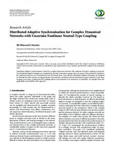
2.1. Detection Model. A network with 𝑁 sensor nodes which are spatially deployed in the ROI is considered. All sensor nodes in this network are independent on functionality. Each sensor makes a decision independently after detection. As illustrated in Figure 1, the sensor nodes which are denoted as symbol of plus are shown to be deployed on a regular grid and intensity of energy attenuated as the distance from the target that is represented as blue star increases. It is worth mentioning that the detection scheme based on harvesting energy is capable of handling any kind of deployment as long as the location information of each sensor node is available at the FC. The uniform sensor deployment shown in Figure 1 is only a special case. In any one kind of deployment, 𝑁 sensor nodes can correctly detect a target when the target intrudes at the position 𝜃 = (𝑥𝑡 , 𝑦𝑡 ), where 𝑥𝑡 and 𝑦𝑡 denote the coordinate of this target location in 2D Cartesian. We introduce an isotropic intensity of signal attenuation model as follows: 𝑎𝑖2 = 𝑃0 (
𝑛
𝑑0 ) , 𝑑E,𝑖
(1)
where 𝑎𝑖 is the signal amplitude received at ith sensor and 𝑃0 is the emitted power measured at a reference distance 𝑑0 . 𝑛 is the power decay exponent, and 𝑑E,𝑖 is the Euclidean distance between the target and ith sensor: 2
2
𝑑E,𝑖 = √(𝑥𝑡 − 𝑥𝑖 ) + (𝑦𝑡 − 𝑦𝑖 ) ,
𝑖 = 1, 2, . . . , 𝑁,
(2)
in which (𝑥𝑖 , 𝑦𝑖 ) are the coordinate of ith sensor. For simplicity but without loss of generality in this paper, we let 𝑛 = 2, 𝑑0 = 1 [10]. As a result, (1) can be expressed as 𝑎𝑖2 =
200
Y-coordinate (m)
metric is also presented. In Section 3, we determine the optimal attacking strategy in the perspective of Byzantine attackers and closed-form expression for blinding region is derived. Comparison among IMBA, CMBA, and NMBA is also performed and numerical results are provided at the same time. From the perspective of network designer, we propose a fusion scheme based on dynamic threshold to make a reliable global decision and analyze how the FC identifies Byzantine attackers to enhance the fusion performance in Section 4. The attacking power is also estimated. Finally, we present our conclusion in Section 5.
𝑃0
2
(𝑑E,𝑖 )
, 𝑖 = 1, 2, . . . , 𝑁.
(3)
Equation (3) is a quite general model for signal attenuation of electromagnetic wave that propagates isotropically in free space. However, when the signal of energy arrives at ith sensor, it has been contaminated by additive white Gaussian noise in practice. Therefore, the signal amplitude received at ith sensor is expressed as 𝑟𝑖 = 𝑎𝑖 + 𝑛𝑖 , in which 𝑛𝑖 is Gaussian noise which follows standard normal distribution. Here, we assume that all sensors in the network have the identical additive white Gaussian noise, that is, 𝑛𝑖 ∼ 𝑁(𝜇, 𝜎2 ), 𝑖 = 1, 2, . . . , 𝑁.
0
0
50
100 X-coordinate (m)
150
200
Figure 1: The sensors are deployed in a regular grid. Each sensor independently harvests the energy propagated from target.
Each sensor node needs to quantize the received signal of energy because of its limitations of bandwidth and energy and sends quantized binary measurements to the FC. Threshold of quantizers is adopted in this work for its simplicity of both easy implementation and analysis as follows: {1, 𝑟𝑖 > 𝜍𝑖 , 𝑑̃𝑖 = { 0, 𝑟𝑖 < 𝜍𝑖 , {
(4)
where 𝑑̃𝑖 and 𝜍𝑖 are local decisions made by ith sensor after quantizing the received signal and a predefined threshold adopted by ith sensor, respectively. In this paper, we assume that all of the sensors share the identical threshold; that is, 𝜍𝑖 = 𝜍, 𝑖 = 1, 2, . . . , 𝑁. In this work, the classical distribution detection model is taken into account where two hypotheses are considered. Each sensor solves hypothesis testing problem and makes a local decision on either hypothesis 𝐻0 (target is absent) or 𝐻1 (target is present). We consider the scenario that the adversary knows the complete information about the location of sensors and is capable of attacking all the sensors simultaneously. Due to the constraint of budget, the Byzantine attackers conquer only a part of nodes in the network to deteriorate capability of inference performance of network. These Byzantine sensors transmit false decision to the FC in order to deteriorate inference performance of the network. We assume that the channel between the FC and local sensors is error-free. The original or local one-bit decision generated at ith sensor node is denoted as 𝑑̃𝑖 ∈ {0, 1}, 𝑖 = 1, 2, . . . , 𝑁. Then the ith sensor reports one-bit decision 𝑑𝑖 to the FC where 𝑑𝑖 = 𝑑̃𝑖 if ith sensor is Honest. For a Byzantine sensor, the local original decision 𝑑𝑖 need not be equal to 𝑑̃𝑖 in our attacks model. Let 𝑁𝐻 and 𝑁𝐵 be the number of Honest and Byzantine sensors, respectively. The total number of sensors can be expressed as 𝑁 = 𝑁𝐻 + 𝑁𝐵 and the number of Byzantine sensor nodes 𝑁𝐵 is equal to 𝛼 ⋅ 𝑁. In the perspective of
4
International Journal of Distributed Sensor Networks
Byzantine attackers, conquering 𝑁 sensors is not a wise strategy for the adversary itself at the risk of exposed activity. The main goal of adversary is to compromise a fraction of sensors to degrade the performance of the FC instead of capturing the network with a huge cost. Therefore, we have 𝑁𝐵 < 𝑁. We use 𝑃𝑑𝐻(𝑖) = Pr(𝑑̃𝑖 = 1 | 𝐻1 , 𝐻) and 𝑃fa𝐻(𝑖) = Pr(𝑑̃𝑖 = 1 | 𝐻0 , 𝐻) to denote the probability of detection and false-alarm of ith sensor, respectively. We use 𝐻 to present a sensor node to be Honest and 𝑖 ∈ {1, 2, . . . , 𝑁𝐻}. The detection probability of ith sensor can be expressed as
(5)
𝜍𝑖 − 𝑎𝑖 − 𝜇 ). 𝜎
Similarly, the false-alarm probability of 𝑖th sensor can be expressed as 𝑃fa𝐻 (𝑖) = Pr (𝑛𝑖 > 𝜍𝑖 ) = 𝑄 (
𝜍𝑖 − 𝜇 ), 𝜎
(6)
where 𝑄(⋅) is the complementary distribution function of the standard Gaussian 𝑄 (𝑥) = ∫
∞
𝑥
1 −𝑡2 /2 𝑑𝑡. 𝑒 √2𝜋
̃1 d
̃2 d
S1
S2 d1
SN−1
···
d2
̃N d
̃ N−1 d
dN−1
SN dN
The fusion center DN×K → z
𝑃𝑑𝐻 (𝑖) = Pr (𝑑̃𝑖 = 1 | 𝐻1 , 𝐻) = Pr (𝑎𝑖 + 𝑛𝑖 > 𝜍𝑖 ) = 𝑄(
Natural state
(7)
When a target intrudes into the ROI, each sensor node starts to sense and record the energy propagated from the target using detection scheme based on harvesting energy [21]. We let each sensor perform 𝐾 observations in a small time window 𝑇 where target is assumed to be static. This is a reasonable assumption. For example, if the sampling rate of each sensor is 6000 Hz, a target with a speed of 100 km/h only moves 0.25 m during 𝑇 = 54 sampling intervals [22]. The jth observation at ith sensor node can be expressed as 𝑑̃𝑖𝑗 , 𝑖 ∈ {1, 2, . . . , 𝑁} and 𝑗 ∈ {1, 2, . . . , 𝐾}. A local/original ̃ ,d ̃ ̃ T ̃ = [d decision matrix D 1 2 , . . . , d𝑁 ] is generated where T ̃ ̃ ̃ ̃ d𝑖 = (𝑑𝑖1 , 𝑑𝑖2 , . . . , 𝑑𝑖𝐾 ) is the vector of local/original decision at the ith sensor node. And 𝑑̃𝑖𝑗 ∈ {0, 1}, 𝑖 ∈ {1, 2, . . . , 𝑁} and 𝑗 ∈ {1, 2, . . . , 𝐾}. The FC receives 𝑁 vectors of decisions from local sensors. Then, a decision matrix D = [d1 , d2 , . . . , d𝑁]T is formulated at the FC; that is, D = (𝑑𝑖𝑗 )𝑁×𝐾 , where 𝑑𝑖𝑗 ∈ {0, 1}, 𝑖 ∈ {1, 2, . . . , 𝑁} and 𝑗 ∈ {1, 2, . . . , 𝐾}. The local/original ̃ is equal to D if there is no presence of decision matrix D Byzantine attackers. In order to formulate the problem in the process of decision fusion, we divide the process into three hierarchies/stages. As illustrated in Figure 2, ith sensor makes a ̃ and sends the vector d into the FC local/original vector of d 𝑖 𝑖 ̃ after d𝑖 is probably “attacked” at the first stage. A decision matrix D is formulated from which the vector of global decision z = (𝑧1 , 𝑧2 , . . . , 𝑧𝐾 ) is mapped at the second stage. At the last stage, a global-final decision 𝑧 is mapped from vector z at the FC. 2.2. Byzantine Attacks Model. In the attacks model of NMBA, the ith Byzantine sensor has exactly 𝑀𝑖 − 1 (𝑖 = 1, 2, . . . , 𝑁𝐵 )
z→z
̃ is the vector of local decision Figure 2: Model of three hierarchies. d 𝑖 made by ith sensor 𝑆𝑖 , d𝑖 is the vector of decision sent to the FC, 𝑖 = 1, 2, . . . , 𝑁. D𝑁×𝐾 is the decision matrix formulated at the FC, z is global decision vector, and 𝑧 is global-final decision.
neighbors to consult and 𝑀𝑖 ≤ 𝑁𝐻. In order to facilitate analysis, we assume that the scenario of many Byzantine sensors flocking together does not happen. Namely, the whole Byzantine sensor nodes are deployed sparsely by intelligent adversary in the ROI. In the case of 𝑁 sensors deployed on a regular grid, NMBA has several neighborhood types including diamond type and square type. For each Byzantine sensor, its neighborhood nodes are those sensors that are the nearest and Honest around it in specific neighborhood type. We assume that each Byzantine sensor knows the identifications of the remaining compromised sensors. Each Byzantine sensor consults all of its neighborhood nodes to make a wise and tricky decision. In Figure 3, the type of square neighborhood is presented and the case of 𝑀𝑖 = 𝑀 = 9 is considered. Clearly, each Byzantine sensor node consults its eight neighbors and makes a decision based on decisions from its neighbors. We make the conditional i.i.d. assumption under which observations from sensors are conditionally independent and identically distributed. The jth observation at ith sensor then has the distributions 𝐻0 : V𝑖𝑗 (𝑘) = Pr (𝑑𝑖𝑗 = 𝑘 | 𝐻0 ) = (1 − 𝛼) Pr (𝑑𝑖𝑗 = 𝑘 | 𝐻0 , 𝐻) + 𝛼 Pr (𝑑𝑖𝑗 = 𝑘 | 𝐻0 , 𝐵) , 𝐻1 : 𝑢𝑖𝑗 (𝑘) = Pr (𝑑𝑖𝑗 = 𝑘 | 𝐻1 ) = (1 − 𝛼) Pr (𝑑𝑖𝑗 = 𝑘 | 𝐻1 , 𝐻) + 𝛼 Pr (𝑑𝑖𝑗 = 𝑘 | 𝐻1 , 𝐵) 𝑖 ∈ {1, 2, . . . , 𝑁} , 𝑗 ∈ {1, 2, . . . , 𝐾} , 𝑘 ∈ {0, 1} .
(8)
International Journal of Distributed Sensor Networks
5 𝑀 −1 is, the original local decision 𝑑̃𝑖𝑗 = IF(∑𝑙=0𝑖 𝑐𝑖𝑙 > 𝜂𝑖 ), where IF(⋅) and 𝜂𝑖 are indicator function and threshold adopted by the ith Byzantine sensor, respectively. Therefore, we have the following equations:
200 180
Y-coordinate (m)
160 140
𝑀𝑖
120
𝑚=𝜂𝑖 𝜋∈Γ 𝑖=1
100
𝑖=𝑚+1
(12)
80
𝑀𝑖
𝑀𝑖
𝑚
𝑥𝑖𝑗 (𝑘) = ∑ ∑ ∏ 𝑝𝜋(𝑖)𝑗 (𝑘) ∏ (1 − 𝑝𝜋(𝑖)𝑗 (𝑘)) ,
60
𝑚=𝜂𝑖 𝜋∈Γ 𝑖=1
40 20 0
𝑀𝑖
𝑚
𝑦𝑖𝑗 (𝑘) = ∑ ∑ ∏ 𝑞𝜋(𝑖)𝑗 (𝑘) ∏ (1 − 𝑞𝜋(𝑖)𝑗 (𝑘)) ,
0
50
100 X-coordinate (m)
150
200
Figure 3: Square type of NMBA in the case of 𝑀. The blue star is a intruding target and symbol plus is denoted as sensor. Byzantine sensors are denoted as plus symbol covered with diamond. Each Byzantine sensor has 9 decisions after consulting its 8 neighborhood nodes.
If ith sensor is Honest, its observation 𝑘 ∈ {0, 1} follows distributions 𝑝 and 𝑞 under hypotheses 𝐻0 and 𝐻1 , respectively. Therefore, we have 𝐻0 : Pr (𝑑̃𝑖𝑗 = 𝑘 | 𝐻0 , 𝐻) = 𝑞𝑖𝑗 (𝑘) ,
𝑖=𝑚+1
where 𝑀𝑖 ∈ {1, 2, . . . , 𝑁𝐻}, 1 ≤ 𝜂 ≤ 𝑀𝑖 , and Γ denotes the set of all permutations of the 𝑀𝑖 sensors. After using majority strategy to make a local decision, the ith Byzantine sensor flips confidently its decision with probability of 𝑃flip = 1. Specifically, we have {1, Pr (𝑑𝑖𝑗 = 𝑘 | 𝑑̃𝑖𝑗 = 𝑙, 𝐵) = { {0,
when 𝑙 ≠ 𝑘 when 𝑙 = 𝑘
(13)
𝑘, 𝑙 ∈ {0, 1} . Thus, we get Pr (𝑑𝑖𝑗 = 𝑘 | 𝐻0 , 𝐵) = ∑ Pr (𝑑̃𝑖𝑗 = 𝑙 | 𝐻0 , 𝐵) 𝑙=𝑘 ̸
𝐻1 : Pr (𝑑̃𝑖𝑗 = 𝑘 | 𝐻1 , 𝐻) = 𝑝𝑖𝑗 (𝑘) ,
(9)
𝑖 = 1, 2, . . . , 𝑁𝐻.
⋅ Pr (𝑑𝑖𝑗 = 𝑘 | 𝑑̃𝑖𝑗 = 𝑙, 𝐻0 , 𝐵) + ∑ Pr (𝑑̃𝑖𝑗 = 𝑙 | 𝐻0 , 𝐵)
According to (5), (6), and (7), we get
𝑙=𝑘
𝜍 − 𝑎𝑖 − 𝜇 𝑝𝑖𝑗 (1) = 𝑄 ( ), 𝜎 𝑝𝑖𝑗 (0) = 1 − 𝑝𝑖𝑗 (1) , 𝜍−𝜇 𝑞𝑖𝑗 (1) = 𝑄 ( ), 𝜎
⋅ Pr (𝑑𝑖𝑗 = 𝑘 | 𝑑̃𝑖𝑗 = 𝑙, 𝐻0 , 𝐵) , (10)
Pr (𝑑𝑖𝑗 = 𝑘 | 𝐻1 , 𝐵) = ∑ Pr (𝑑̃𝑖𝑗 = 𝑙 | 𝐻1 , 𝐵)
(14)
𝑙=𝑘 ̸
⋅ Pr (𝑑𝑖𝑗 = 𝑘 | 𝑑̃𝑖𝑗 = 𝑙, 𝐻1 , 𝐵)
𝑞𝑖𝑗 (0) = 1 − 𝑞𝑖𝑗 (1) . Similarly, we have distributions 𝑥 and 𝑦 under the same hypotheses for Byzantine sensor as follows: 𝐻0 : Pr (𝑑̃𝑖𝑗 = 𝑘 | 𝐻0 , 𝐵) = 𝑦𝑖𝑗 (𝑘) ,
+ ∑ Pr (𝑑̃𝑖𝑗 = 𝑙 | 𝐻1 , 𝐵) 𝑙=𝑘
⋅ Pr (𝑑𝑖𝑗 = 𝑘 | 𝑑̃𝑖𝑗 = 𝑙, 𝐻1 , 𝐵) .
𝐻1 : Pr (𝑑̃𝑖𝑗 = 𝑘 | 𝐻1 , 𝐵) = 𝑥𝑖𝑗 (𝑘) ,
(11) 𝑖 = 1, 2, . . . , 𝑁𝐵 .
In the attacks model of NMBA, the ith Byzantine sensor makes an initial decision 𝑐𝑖0 independently and gets the 𝑀𝑖 −1 decisions from its neighborhood sensors. As a result, a set of decisions {𝑐𝑖𝑙 : 𝑙 ∈ {0, 1, . . . , 𝑀𝑖 − 1}, 𝑐𝑖𝑙 ∈ {0, 1}} is obtained where the 𝑐𝑖𝑙 represents the decision from the lth neighbor of ith Byzantine sensor. Then, the ith Byzantine sensor makes its local or original decision using a majority strategy, that
Therefore, we have Pr (𝑑𝑖𝑗 = 0 | 𝐻0 , 𝐵) = Pr (𝑑̃𝑖𝑗 = 1 | 𝐻0 , 𝐵) = 𝑦𝑖𝑗 (1) , Pr (𝑑𝑖𝑗 = 1 | 𝐻0 , 𝐵) = Pr (𝑑̃𝑖𝑗 = 0 | 𝐻0 , 𝐵) = 𝑦𝑖𝑗 (0) , Pr (𝑑𝑖𝑗 = 0 | 𝐻1 , 𝐵) = Pr (𝑑̃𝑖𝑗 = 1 | 𝐻1 , 𝐵) = 𝑥𝑖𝑗 (1) , Pr (𝑑𝑖𝑗 = 1 | 𝐻1 , 𝐵) = Pr (𝑑̃𝑖𝑗 = 0 | 𝐻1 , 𝐵) = 𝑥𝑖𝑗 (0) .
(15)
6
International Journal of Distributed Sensor Networks
Substituting (9) and (15) in (8) and after simplification, we obtain V𝑖𝑗 (𝑘) = Pr (𝑑𝑖𝑗 = 𝑘 | 𝐻0 )
Substituting (16) in (18) and after simplification, the condition to make KLD(V𝑖𝑗 (𝑘) ‖ 𝑢𝑖𝑗 (𝑘)) = 0 is equivalent to 𝛼=
= (1 − 𝛼) [𝑘𝑞𝑖𝑗 (𝑘) + (1 − 𝑘) (1 − 𝑞𝑖𝑗 (𝑘))] =
+ 𝛼𝑦𝑖𝑗 (1 − 𝑘) ,
(16)
𝑢𝑖𝑗 (𝑘) = Pr (𝑑𝑖𝑗 = 𝑘 | 𝐻1 )
𝑝𝑖𝑗 (1) − 𝑞𝑖𝑗 (1) (𝑝𝑖𝑗 (1) − 𝑞𝑖𝑗 (1)) + (𝑥𝑖𝑗 (1) − 𝑦𝑖𝑗 (1)) (𝑝𝑖𝑗 (1) − 𝑞𝑖𝑗 (1)) + 𝑓 (𝑀𝑖 , 𝜂𝑖 , 𝑝𝑖𝑗 (1) , 𝑞𝑖𝑗 (1))
𝑓 (𝑀𝑖 , 𝜂𝑖 , 𝑝𝑖𝑗 (1) , 𝑞𝑖𝑗 (1))
+ 𝛼𝑥𝑖𝑗 (1 − 𝑘) .
𝑀𝑖
2.3. Performance Metric. In the perspective of Byzantine attackers, the primary objective is to deteriorate the inference performance of FC as much as possible. On the contrary, the FC wants to make inference performance as much highly excellent as possible in order to guarantee valid detection. In this paper, we adopt Kullback-Leibler divergence (KLD) as the network performance that characterizes inference performance at the FC. KLD is very important in probability theory and is widely employed as information-theoretic distance measure to characterize detection performance [23, 24]. The KLD between the distributions V𝑖𝑗 (𝑘) = Pr(𝑑𝑖𝑗 = 𝑘 | 𝐻0 ) and 𝑢𝑖𝑗 (𝑘) = Pr(𝑑𝑖𝑗 = 𝑘 | 𝐻1 ) for ith sensor can be expressed as
𝑘∈{0,1}
𝑢𝑖𝑗 (𝑘) V𝑖𝑗 (𝑘)
.
(17)
The FC receives ith sensor’s decisions V𝑖𝑗 (𝑘) and 𝑢𝑖𝑗 (𝑘) under 𝐻0 and 𝐻1 , respectively. In the perspective of Byzantine attackers, they try to minimize the KLD as much as possible so that the FC can hardly make a right decision between 𝐻0 and 𝐻1 . On the other hand, network designer wants to maximize KLD of each sensor’s decision to mitigate the negative effect caused by Byzantine attackers. In the next section, we explore the optimal strategy of Byzantine attacks that impair the detection performance as much as possible by minimizing KLD.
3. Optimal Strategy for Byzantine Attackers
𝑢𝑖𝑗 (𝑘) = Pr (𝑑𝑖𝑗 = 𝑘 | 𝐻1 ) = Pr (𝑑𝑖𝑗 = 𝑘 | 𝐻0 )
(18)
𝑀𝑖
𝑚
= ∑ ∑ ∏ 𝑝𝜋(𝑖)𝑗 (1) ∏ (1 − 𝑝𝜋(𝑖)𝑗 (1)) 𝑚=𝜂𝑖 𝜋∈Γ 𝑖=1 𝑀𝑖
(20)
𝑖=𝑚+1
𝑀𝑖
𝑚
− ∑ ∑ ∏ 𝑞𝜋(𝑖)𝑗 (1) ∏ (1 − 𝑞𝜋(𝑖)𝑗 (1)) , 𝑚=𝜂𝑖 𝜋∈Γ 𝑖=1
𝑖=𝑚+1
where 𝑀𝑖 and 𝜂𝑖 are the number of neighborhood nodes and threshold adopted by ith Byzantine sensor, respectively. As mentioned above, the KL distance between V𝑖𝑗 (𝑘) and 𝑢𝑖𝑗 (𝑘) is equal to zero; that is, KLD(V𝑖𝑗 ‖ 𝑢𝑖𝑗 ) = 0, if and only if V𝑖𝑗 (𝑘) = 𝑢𝑖𝑗 (𝑘). The FC is incapable of distinguishing the two distributions under 𝐻0 and 𝐻1 when KLD is equal to zero. The attackers then project interests in the minimum attacking power that can just make the ability of inference of the FC destroyed. Thus, the minimum attacking power in the context of NMBA is denoted as 𝛼blind = min {𝛼; 𝛼 that make KLD (𝑢𝑖𝑗 ‖ V𝑖𝑗 ) = 0} .
(21)
For the sake of minimizing 𝛼 to reach 𝛼blind , we have the following equation depending on operating point (𝑝𝑖𝑗 (1), 𝑞𝑖𝑗 (1)): 𝛼blind =
𝑝𝑖𝑗 (1) − 𝑞𝑖𝑗 (1) (𝑝𝑖𝑗 (1) − 𝑞𝑖𝑗 (1)) + max {𝑓 (𝑀𝑖 , 𝜂𝑖 , 𝑝𝑖𝑗 (1) , 𝑞𝑖𝑗 (1))}
.
(22)
Because of 0 < 𝑝𝑖𝑗 (1) − 𝑞𝑖𝑗 (1) ≤ 1, we have the following inequality: 𝛼blind ≤
3.1. Optimal Strategy for Byzantine Attacks. As explored in Section 2, the Byzantine attackers attempt to make the nodes that have been compromised have small KL divergence as much as possible. Byzantine attackers have the optimal superiority on degrading inference performance of FC when KLD is equal to zero. In the case of KLD = 0, the FC cannot distinguish the distributions under 𝐻0 or 𝐻1 . In other words, the data from sensors conveys no information. We refer to this case as the FC being blinded completely when
= V𝑖𝑗 (𝑘) .
,
where the close-form expression of function 𝑓(⋅) is denoted as the following equation:
= (1 − 𝛼) [𝑘𝑝𝑖𝑗 (𝑘) + (1 − 𝑘) (1 − 𝑝𝑖𝑗 (𝑘))]
KLD (𝑢𝑖𝑗 ‖ V𝑖𝑗 ) = ∑ 𝑢𝑖𝑗 (𝑘) log
(19)
𝑝𝑖𝑗 (1) − 𝑞𝑖𝑗 (1)
1 1 + max {𝑓 (𝑀𝑖 , 𝜂𝑖 , 𝑝𝑖𝑗 (1) , 𝑞𝑖𝑗 (1))}
.
(23)
To prove inequality (23), we apply the monotonic property of the function of 𝑥/(𝑥 + 1). Due to the function possessing differentiability, we have the following inequality: 𝑑 𝑥 1 > 0. ( )= 𝑑𝑥 𝑥 + 1 (𝑥 + 1)2
(24)
Therefore, 𝑥/(𝑥 + 1) is a monotonically increasing function when 0 ≤ 𝑥 ≤ 1. As a result, inequality (23) is certified. After certifying (23), we have the following equation: 𝜂𝑖 opt = ceil (
𝑀𝑖 ), 2
(25)
International Journal of Distributed Sensor Networks
7
0.9
5
0.8
4.5 4
0.7
3.5
0.6
3 𝜂opt
𝛼
0.5 0.4
2.5 2
0.3
1.5
0.2
1
0.1
0.5
0
0 1
2
3
4
5
6
7
8
9
Figure 4: Attacking power 𝛼 versus 𝜂 when 𝑀 = 9, 𝜂 varying from 1 to 9. Byzantine sensors have the smallest 𝛼 when 𝜂 = 5.
where ceil(⋅) is the ceiling function. Therefore, function 𝑓(⋅) in (19) reaches the maximum value point only when 𝜂𝑖 = 𝜂𝑖 opt . Therefore, for a pair of fixed operating points (𝑝𝑖𝑗 (1), 𝑞𝑖𝑗 (1)), we have max 𝑓 = 𝑓 (𝑀𝑖 , ceil (
𝑀𝑖 ) , 𝑝𝑖𝑗 (1) , 𝑞𝑖𝑗 (1)) 2
(26)
and (22) can be represented as 𝛼blind =
𝑝𝑖𝑗 (1) − 𝑞𝑖𝑗 (1) (𝑝𝑖𝑗 (1) − 𝑞𝑖𝑗 (1)) + max 𝑓
1
2
3
4
5
6
7
8
9
M
𝜂
.
(27)
When the intelligent adversary poses attacking power 𝛼 which is greater than 𝛼blind , the FC is trapped into a dilemma where the decider cannot utilize any information from sensors to make a correct decision. The situation refers to the fusion center’s entering into the blinding region where the FC is blinded completely. 3.2. Numerical Results. In this subsection, numerical results are presented to support our analysis of optimal attacking strategy for Byzantine attackers. We consider the network where 𝑁 = 100 sensors are deployed on regular grid in the ROI under the Byzantine attacks model of NMBA. We set the power at the reference point (𝑑0 = 1) as 200 and the signal amplitude arriving at the local sensor is contaminated by AWGN with mean value 𝜇 = 0 and standard deviation 𝜎 = 3. A target intrudes at position 𝜃 = (90, 90). We consider the square type of NMBA where all the Byzantine sensors adopt identical number of neighborhood nodes and optimal threshold; that is, 𝑀 = 𝑀𝑖 and 𝜂 = 𝜂𝑖 opt , 𝑖 = 1, 2, . . . , 𝑁𝐵 . Attacking power 𝛼 is observed in the case of square type of NMBA over 𝑀 ∈ {1, 2, . . . , 𝑁𝐻} and 𝜂 ∈ {1, 2, . . . , 𝑀}. In the blinding region, the FC is incapable of utilizing any information to make a decision to determine whether there is a target in the ROI. Byzantine users try to pay as much low cost as possible when the FC has been completely blinded by them. Attacking power 𝛼 in blinding region is a convex function of threshold 𝜂
Figure 5: Optimal threshold 𝜂 versus 𝑀, 𝑀 varying from 1 to 9. The optimal threshold increases with the increment of 𝑀 and it is always equal to ceil(𝑀/2).
under the NMBA attacking model. Therefore, it is possible for Byzantine attackers to adopt the least attacking power to blind the FC. From the numerical results presented in Figure 4, we see that the attacking power 𝛼 reaches minimum value only when 𝜂 = 5 in the case of NMBA when 𝑀 = 9. The minimum value of 𝛼 is equal to 0.3844. The result is intuitive and also indicates that the optimal threshold associates with the number of neighborhood nodes, 𝑀. The other cases of NMBA are presented in Table 1. We observe that the minimum value of 𝛼blind is just obtained at the point where the optimal threshold 𝜂 is got. In Figure 5, we present that optimal threshold increases with the increase in the value of 𝑀. We observe that 𝜂opt is always equivalent to 𝑀/2 when 𝑀 is even and 𝜂opt is equal to the maximum integer that is not larger than 𝑀/2 when 𝑀 is odd. It is clear that optimal threshold Byzantine attacker associates with the number of its neighborhood. In Figures 6 and 7, it is shown that 𝛼blind is the monotonically decreasing function of 𝑀 in the condition that 𝜂 is always equal to 𝜂opt . As illustrated in Figures 5 and 6, IMBA is a particular case when 𝑀 = 1. Under condition of 𝑀 = 1, each Byzantine sensor makes a judgement only depending on its own observation and flips its decision confidently prior to sending to the FC. When 𝑀 = 2, each Byzantine sensor consults with two neighborhood nodes around it before making a decision and the minimum attacking power in the blinding region is equal to 0.5. When 𝑀 is equal to 2, the attacking effect brought by NMBA matches with IMBA. 𝛼blind of NMBA decreases monotonically with the increase of 𝑀 and it reaches 0.3844 when 𝑀 increases to 9. 𝛼blind decreases to 0.3752 when 𝑀 increases to 25. The exact value of 𝛼blind corresponding to 𝑀 and 𝜂opt is presented in Table 2. In addition, as we can see from Figures 6 and 7, the number of neighborhood nodes that each Byzantine sensor node consults including itself should be odd for better attacking efficiency. To further analyze the attacks of NMBA, we compare it with IMBA and CMBA in terms of KL distance about attacking power. As we discussed above, IMBA is a special case of NMBA when 𝑀 = 1.
8
International Journal of Distributed Sensor Networks Table 1: 𝛼 at (𝑀, 𝜂), 𝑀 ∈ {1, 2, . . . , 9} and 𝜂 ≤ 𝑀.
1 2 3 4 5 6 7 8 9
1 0.5000 0.5000 0.5434 0.5952 0.6469 0.6959 0.7410 0.7814 0.8171
2
3
4
𝜂 5
6
7
8
9
0.5000 0.4310 0.4310 0.4509 0.4785 0.5100 0.5438 0.5790
0.5434 0.4310 0.4042 0.4042 0.4145 0.4298 0.4484
0.5952 0.4509 0.4042 0.3913 0.3913 0.3970
0.6469 0.4785 0.4145 0.3913 0.3844
0.6959 0.5100 0.4298 0.3970
0.7410 0.5438 0.4484
0.7814 0.5790
0.8171
𝐿 out of 𝑁𝐵 fusion rule has been used for CMBA among the Byzantine sensors. And Byzantine sensors collaborate together to make decisions about the presence of target. If the attacking power is greater than 0.5, the FC can be blinded completely by any kinds of attacking strategies adopted by Byzantine attackers. Therefore, our analysis about detection performance is under the condition of 𝛼 ≤ 0.5. In Figures 8 and 9, we plot the KLD of three attacking models against 𝛼 in the case 𝑀 = 9 and 𝑀 = 25, respectively. From the numerical results presented in Figures 8 and 9, we can see that the KLD of NMBA is very close to CMBA and outperforms IMBA significantly. Though the performance of NMBA is very close to CMBA, the difference of KL distance between them varies with attacking power. In Figures 8 and 9, KL distance of CMBA is greater than that of NMBA in the region of 𝛼 ∈ [0, 0.09] and 𝛼 ∈ [0, 0.25], respectively. However, CMBA performs better when 𝛼 meets the condition of 𝛼 ≥ 0.09 and 𝛼 ≥ 0.025 in Figures 8 and 9, respectively. For CMBA, the blinding point C which is marked by black-square in Figures 8 and 9 is determined by the total number of Byzantine sensor nodes instead of 𝑀. For NMBA, the blinding point B which is marked by blue-square in Figures 8 and 9 is determined by the number of neighborhood nodes. For NMBA, 𝑀 is larger and 𝛼blind is smaller. Furthermore, 𝛼blind = 0.3844 and 𝛼blind = 0.3751 when 𝑀 is equal to 9 and 25, respectively.
0.5 0.45 0.4 0.35 0.3 𝛼blind
𝑀/𝛼
0.2 0.15 0.1 0.05 0
1
2
3
4
5
6
7
8
9
M
Figure 6: 𝛼blind versus 𝑀, 𝑀 varying from 1 to 9 in condition of 𝜂 = 𝜂opt . 𝛼blind monotonically decreases with 𝑀. It is clear that Byzantine attacker more easily blinds the FC when each Byzantine sensor has more neighborhood nodes.
0.5 0.45 0.4
4. Fusion Center Decision Strategy
0.35 0.3 𝛼blind
In this section, let us solve the problem of identifying Byzantine attackers to enhance inference performance of the FC. In order to explain the problem well, we have defined three types of decision which include local/original decision, global decision, and global-final decision. As we discussed in Section 2, a decision matrix D𝑡𝑁×𝐾 = (𝑑𝑖𝑗 (𝑡))𝑁×𝐾 is formulated at the FC after 𝐾 observations in a time window 𝑇 at tth global-final decision making, 𝑡 ∈ 𝑁+ . We let the FC make a corresponding global decision 𝑧𝑗 (𝑡) over vector of decision d𝑡𝑗 at jth observation. And a vector of global decision z(𝑡) = (𝑧1 (𝑡), 𝑧2 (𝑡), . . . , 𝑧𝐾 (𝑡)) is formulated over {d𝑡1 , d𝑡2 , . . . , d𝑡𝐾 }, 𝑧𝑗 (𝑡) ∈ {0, 1} for any 𝑡 ∈ 𝑁+ , 𝑗 = 1, 2, . . . , 𝐾. Majority vote which is simple and effective scheme is adopted to make a global-final decision 𝑧(𝑡) ∈ {0, 1} over the vector z(𝑡), where “1” represents the presence of target and “0”
0.25
0.25 0.2 0.15 0.1 0.05 0
1
3
5
7
9 11 13 15 17 19 21 23 25 M
Figure 7: 𝛼blind versus 𝑀, 𝑀 varying from 1 to 25 in condition of 𝜂 = 𝜂opt . 𝛼blind monotonically decreases with 𝑀. It is clear that Byzantine attacker more easily blinds the FC when each Byzantine sensor has more neighborhood nodes.
International Journal of Distributed Sensor Networks
9
Table 2: 𝛼blind at (𝑀, 𝜂opt ), 𝑀 ∈ {1, 2, . . . , 9} and 𝜂opt = ceil(𝑀/2). 1/1 0.5000
2/1 0.5000
3/2 0.4310
4/2 0.4310
5/3 0.4042
1.4
1.4
1.2
1.2
1
1
0.8
0.8
KLD(𝛼)
KLD(𝛼)
𝑀/𝜂opt 𝛼blind
0.6
0.4
0.2
0.2 C 0
0.1
0.2
0.3
B 0.4
A 0.5
7/4 0.3913
8/4 0.3913
9/5 0.3844
0.6
0.4
0
6/3 0.4042
0
C 0
0.1
0.2
0.3
B 0.4
A 0.5
Attacking power: 𝛼
Attacking power: 𝛼
IMBA NMBA CMBA
IMBA NMBA CMBA
Figure 8: KLD decreases monotonically with attacking power 𝛼 when 𝑀 = 9. KLD of IMBA decreases to 0 when 𝛼 = 0.5. KLD of NMBA decreases to 0 when 𝛼 = 0.3844 in the condition of 𝜂 = 𝜂opt . KLD of CMBA decreases to 0 when 𝛼 = 0.35.
represents the absence of target, respectively. However, we project our focus on designing a rule to construct vector of global decision z(𝑡). We propose a scheme of making global decision that the FC can adaptively adjust its threshold 𝜂fc (𝑡, 𝑗) for d𝑡𝑗 to make a corresponding global decision 𝑧𝑗 (𝑡). The information of elements in decision matrix D𝑡𝑁×𝐾 is also utilized to estimate probability of miss detection and false alarm, respectively. In order to evaluate the fusion scheme, performance metric introduced in this work is the accuracy of fusion scheme in terms of identifying Byzantine sensors. We define an intuitive distance between the global-final decision and local/original decisions as 𝑡 𝑁 d𝑗 = ∑ 𝑑𝑖𝑗 (𝑡) − 𝑧 (𝑡) .
(28)
𝑖=1
Similarly, another intuitive distance is also defined as the following equation: 𝑡 𝐾 d𝑖 = ∑ 𝑑𝑖𝑗 (𝑡) − 𝑧 (𝑡) .
(29)
𝑗=1
In (29), |d𝑡𝑖 | measures the degree of discrepancy between the global-final decision and 𝐾 local/original decisions that are from ith sensor. Similarly, |d𝑡𝑗 | in (28) measures the degree of discrepancy between the global-final decision and 𝑁 local/original decisions generated at jth observation. The
Figure 9: KLD decreases monotonically with attacking power 𝛼 when 𝑀 = 25. KLD of IMBA decreases to 0 when 𝛼 = 0.5. KLD of NMBA decreases to 0 when 𝛼 = 0.3752 in the condition of 𝜂 = 𝜂opt . KLD of CMBA decreases to 0 when 𝛼 = 0.35.
distance |d𝑡𝑖 | is larger and the ith sensor is closer to behavior of Byzantine. On the contrary, the distance of |d𝑡𝑖 | is smaller and the probability of ith sensor being tagged as Byzantine attacker by the FC is lower. Similarly, when the distance of |d𝑡𝑗 | is larger, the decision generated at jth observation is worse. The FC regards the jth observation as excellent and we believe that the network performs well when |d𝑡𝑗 | is small. For simplicity, we let probability of miss detection equal probability of false alarm; that is, 𝑃𝑚 = 𝑃fa in the context of the attacks model of NMBA. 4.1. Scheme of Identifying Byzantine Attackers. If one sensor’s local/original decision is different from global-final decision, it is labeled as Byzantine. It is worth mentioning that Honest sensors are classified probably into Byzantine group when they behave like Byzantine. Similarly, the Byzantine attackers can also be probably labeled as Honest. We use 𝑁0 (𝑡, 𝑗) and 𝑁1 (𝑡, 𝑗) to denote the total effective number of elements “0” and “1” in decision matrix, respectively. 𝑁0 (𝑡, 𝑗) and 𝑁1 (𝑡, 𝑗) vary with the order of 𝑗 and take part in making global decision. Here, we represent (28) and (29) again as follows: d𝑡 = ∑ 𝑑 (𝑡) − 𝑧 (𝑡) , 𝑖𝑗 𝑗 𝑖∈𝐼(𝑡,𝑗)
𝑡 𝐾 d𝑖 = ∑ 𝑑𝑖𝑘 (𝑡) − 𝑧 (𝑡) , 𝑘=1
where 𝐼(𝑡, 𝑗) is defined at (37).
(30) 𝑖 ∈ 𝐼 (𝑡, 𝑗) ,
10
International Journal of Distributed Sensor Networks
Proposition 1. Suppose the network with 𝑁 sensors including Byzantine and Honest, where the probability of miss detection and false-alarm is zero, that is, 𝑃𝑚 = 𝑃𝑓𝑎 = 0, and Byzantine attackers always know the true natural state. Attacking power brought by the attackers is estimated through the following expression: 𝛼̂ (𝑡) =
min {𝑁0 (𝑡) , 𝑁1 (𝑡)} , 𝑁
(31)
where 𝑁0 (𝑡) and 𝑁1 (𝑡) are denoted as the total number of “0” and “1,” respectively. Proof. See Appendix A. Based on Proposition 1 and constrained by its conditions, we have the following equation for estimating the attacking power at the global decision making: 𝛼̂ (𝑡, 𝑗) =
min {𝑁0 (𝑡, 𝑗) , 𝑁1 (𝑡, 𝑗)} . 𝑁0 (𝑡, 𝑗) + 𝑁1 (𝑡, 𝑗)
(32)
Taking the scenario of Byzantine attackers without knowledge about true natural state into consideration in practical application, we have the following. Proposition 2. Suppose the network of size 𝑁 containing both Honest sensors and Byzantine sensor nodes, where decision matrix D𝑡𝑁×𝐾 is made at tth global-final decision after 𝑁 sensors taking 𝐾 observations in the time window 𝑇. The network is not completely blinded by adversary. The estimation of least attacking power has a lower bound which can be expressed as 𝛼̂ (𝑡, 𝑗) ≥
min {𝑁0 (𝑡, 𝑗) , 𝑁1 (𝑡, 𝑗)} − 𝐾 ⋅ [max𝑘 (d𝑡𝑘 ) − min𝑘 (d𝑡𝑘 )] , (33) 𝑛 (𝑡, 𝑗) ⋅ 𝐾 𝑘 ∈ {1, 2, . . . , 𝐾} .
It is clear that 𝛼̂(𝑡, 0) = 0 and 𝑛(𝑡, 0) = 𝑁, 𝑡 ∈ 𝑁+ . In (33), [max𝑘 (|d𝑡𝑘 |) − min𝑘 (|d𝑡𝑘 |)] is used to compute the maximum distance of decisions between two certain vectors of observation which are from two sensors tagged as Honest at the (𝑗 − 1)th global decision making. Proof. See Appendix B. Here, we let 𝛼̂ (𝑡, 𝑗) min {𝑁0 (𝑡, 𝑗) , 𝑁1 (𝑡, 𝑗)} − 𝐾 ⋅ [max𝑗 (d𝑡𝑗 ) − min𝑗 (d𝑡𝑗 )] (34) = 𝑛 (𝑡, 𝑗) ⋅ 𝐾
during the process of identifying Byzantine sensors. After estimating the attacking power, 𝛼̂(𝑡, 𝑗), the FC approximately knows how many sensors have been compromised by an adversary among 𝑛(𝑡, 𝑗) sensors that participate in the jth global decision making. The FC then takes an action to identify 𝛼̂(𝑡, 𝑗) ⋅ 𝑛(𝑡, 𝑗) Byzantine sensors to help the next global decision making. 𝐿(𝑡, 𝑗) is defined as the set of identities of
sensors that are tagged as Honest at the (𝑗−1)th. These sensors will participate in the jth global decision making. It is clear that 𝐿(𝑡, 0) = {𝑖 ‖ 𝑖 = 1, 2, . . . , 𝑁}, 𝑡 ∈ 𝑁+ . We define a sequence 𝐼𝑁(𝑡, 𝑗) over {|d𝑡𝑖 | | 𝑖 ∈ 𝐿(𝑡, 𝑗 − 1)}, in which |d𝑡𝑖 |𝑚 is used for presenting the element with order 𝑚, 𝑚 ∈ {1, 2, . . . , 𝑛(𝑡, 𝑗)}. If |d𝑡𝑖 |𝑚 > |d𝑡𝑙 |𝑛 , then 𝑚 > 𝑛. The identity 𝑖 is greater than 𝑙 when 𝑚 > 𝑛 if |d𝑡𝑖 |𝑚 = |d𝑡𝑙 |𝑛 or 𝑖 < 𝑙 when 𝑚 < 𝑛; otherwise, 𝑖, 𝑙 ∈ 𝐿(𝑡, 𝑗 − 1), 𝑚, 𝑛 ∈ {1, 2, . . . , 𝑛(𝑡, 𝑗)}. The sequence can be expressed as 𝐼𝑁 (𝑡, 𝑗) (35) 1 𝑛(𝑡,𝑗) 𝑡 𝑛(𝑡,𝑗)−1 , d𝑖 , . . . , d𝑡𝑖 | 𝑖 ∈ 𝐿 (𝑡, 𝑗 − 1)} , = {d𝑡𝑖 where ∀𝑚 ∈ {1, 2, . . . , 𝑛(𝑡, 𝑗)}, |d𝑡𝑖 |𝑚 matches only a specific identity. There are 𝑛(𝑡, 𝑗) identities and |𝐼𝑁(𝑡, 𝑗)| = 𝑛(𝑡, 𝑗). In order to find the sequence of d𝑡𝑖 , we define a function ID(⋅) over 𝐼𝑁(𝑡, 𝑗): 𝑛 = ID (d𝑡𝑖 ) =
∑ 𝑙∈𝐿(𝑡,𝑗−1)
+
𝑛 IF (d𝑡𝑙 > d𝑡𝑖 )
∑ 𝑙∈𝐿(𝑡,𝑗−1)
𝑛 IF (d𝑡𝑙 = d𝑡𝑖 | 𝑙 > 𝑗) ,
(36)
𝑛 ∈ {1, 2, . . . , 𝑛 (𝑡, 𝑗)} , where IF(⋅) is an indicator function, and IF(true) = 1 and IF(false) = 0. The FC have obtained the approximate knowledge about the attacking power posed by the adversary at jth global decision making. The FC has also known each sensor’s sequence in 𝐼𝑁(𝑡, 𝑗). Therefore, sensors whose sequences are dropped into the region from 𝑛(𝑡, 𝑗) to {𝑛(𝑡, 𝑗) ⋅ [1 − 𝛼̂(𝑡, 𝑗)] + 1} are judged to be Byzantine attackers. The decisions from Byzantine attackers are removed at the (𝑗 + 1)th global decision making. The identities of remaining sensors which are trusted by the FC at jth global decision making can be expressed as 𝐼 (𝑡, 𝑗) = {𝑖 | ID (d𝑡𝑖 ) < 𝛼̂ (𝑡, 𝑗) ⋅ 𝑛 (𝑡, 𝑗) , 𝑖 ∈ 𝐿 (𝑡, 𝑗 − 1)}
(37)
and 𝐼(𝑡, 𝑗) ⊆ 𝐿(𝑡, 𝑗−1). The attacking power at tth global-final decision making is estimated by the following equation: 𝛼̂ (𝑡) =
𝑁 − 𝑛 (𝑡, 𝐾) . 𝑁
(38)
4.2. Rule of Decision Fusion Based on Dynamic Threshold. As we described in Section 2, the process of making a globalfinal decision is divided into three stages. A local/origĩ𝑡 nal decision matrix D 𝑁×𝐾 is generated at the first stage. A 𝑡 ̃𝑡 decision matrix D𝑁×𝐾 is formulated after D 𝑁×𝐾 being probably attacked. A vector of global decision z(𝑡) = (𝑧1 (𝑡), 𝑧2 (𝑡), . . . , 𝑧𝐾 (𝑡)) is computed and obtained over vectors of decision {d𝑡1 , d𝑡2 , . . . , d𝑡𝐾 } through applying a policy of fusion
International Journal of Distributed Sensor Networks
11
at the middle stage. At last, the decider at the FC has a global-final decision 𝑧(𝑡). In this paper, we put our focus on proposing an effective method of decision fusion to get an excellent vector of global decision z(𝑡), which can easily help to make a global-final decision 𝑧(𝑡) at the last stage. The rule of decision fusion based on dynamic threshold is that threshold (𝜂fc (𝑡, 𝑗)) for jth global decision making varies with 𝑗. The number of sensors which participate in jth global decision making is denoted as 𝑛(𝑡, 𝑗). In addition, 𝑛(𝑡, 𝑗) always associates with 𝑛(𝑡, 𝑗 − 1) tightly, which is expressed as 𝑛 (𝑡, 𝑗) = 𝑛 (𝑡, 𝑗 − 1) ⋅ [1 − 𝛼̂ (𝑡, 𝑗 − 1)] .
(39)
Here, 𝑞 out of 𝑚 fusion rule in [13] has been used for designing threshold 𝜂fc (𝑡, 𝑗), which is given by 𝜂fc (𝑡, 𝑗) = floor (𝑎 ⋅ 𝑛 (𝑡, 𝑗) + √𝑏 ⋅ 𝑛 (𝑡, 𝑗)𝑄−1 (1 − 𝛽)) ,
(40)
where floor(⋅) is a floor function and 𝑄−1 (⋅) is the inverse function of 𝑄(⋅) which has been introduced in Section 2. 𝛽 is a predefined constraint of miss detection. 𝑎 and 𝑏 are given by 𝑎 = [1 − 𝛼̂ (𝑡, 𝑗)] ⋅ 𝑝𝑖𝑗 (1) + 𝛼̂ (𝑡, 𝑗) ⋅ 𝑥𝑖𝑗 (1) , 𝑏 = [1 − 𝛼̂ (𝑡, 𝑗)] ⋅ 𝑝𝑖𝑗 (1) ⋅ (1 − 𝑝𝑖𝑗 (1)) + 𝛼̂ (𝑡, 𝑗) ⋅ 𝑦𝑖𝑗 (1) ⋅ (1 − 𝑦𝑖𝑗 (1)) ,
(41) (42)
respectively. Therefore, we get the jth global decision 𝑧𝑗 (𝑡): 𝑧𝑗 (𝑡) = IF (∑ 𝑑𝑖𝑗 (𝑡) > 𝜂fc (𝑡, 𝑗) | 𝑖 ∈ 𝐿 (𝑡, 𝑗 − 1)) .
(43)
𝑖
In order to evaluate the identifying scheme, we define 𝛾𝐻𝐻, 𝛾𝐻𝐵 , 𝛾𝐵𝐻, and 𝛾𝐵𝐵 as the accuracy of identifying Byzantine attackers. 𝛾𝐻𝐻 and 𝛾𝐻𝐵 are formulated as accuracy of Honest sensors tagged as Honest and Byzantine, respectively. Similarly, 𝛾𝐵𝐻 and 𝛾𝐵𝐵 are defined as accuracy of Byzantine sensors identified as Honest and Byzantine, respectively. We have the equations as follows: 𝛾𝐻𝐵 =
𝑁𝐻𝐵 , 𝑁
𝛾𝐻𝐻 =
𝑛 (𝑡, 𝐾) − 𝑁𝐵𝐻 , 𝑁
𝛾𝐵𝐻
𝑁 = 𝐵𝐻 , 𝑁
𝛾𝐵𝐵 =
(44)
𝑁 − 𝑛 (𝑡, 𝐾) − 𝑁𝐻𝐵 . 𝑁
Therein, 𝑁𝐻𝐵 is the number of Honest sensors identified as Byzantine and the number of Byzantine sensors identified as Honest is denoted as 𝑁𝐵𝐻. 𝑁𝐻 and 𝑁𝐵 have been described in Section 2.
4.3. Numerical Results. In this subsection, we analyze the performance of scheme of identifying Byzantine attackers through numerical results. There are also 100 sensor nodes that contain Byzantine and Honest nodes which are considered in our simulation. Meanwhile, global-final decision making is performed 100 times in our simulation. The power at the reference point (𝑑0 = 1) is set as 200 and the signal amplitude arriving at the local sensor has been contaminated by AWGN with mean value 𝜇 = 0 and standard deviation 𝜎 = 3. A target intrudes at position 𝜃 = (90, 90). The true attacking power is fixed to 0.3 and 𝛽 = 0.2. In Figures 10, 11, 12, and 13, we show that 𝑛(𝑡, 𝑗) decreases following the increase of 𝑗 and has stable tendency to a fixed level. The sum of 𝑁0 (𝑡, 𝑗) and 𝑁1 (𝑡, 𝑗) is always equal to 𝐾 ⋅ 𝑛(𝑡, 𝑗) and 𝑁1 (𝑡, 𝑗) is greater than 𝑁0 (𝑡, 𝑗). 𝑁0 (𝑡, 𝑗) and 𝑁1 (𝑡, 𝑗) verge to 𝐾⋅𝑁𝐵 and 𝐾⋅𝑁𝐻, respectively. And 𝛼̂(𝑡, 𝑗) → 0 when 𝑗 exceeds a certain number and 𝛼̂(𝑡, 𝑗) = 0 when 𝑗 ≥ 7 in the scheme of identifying Byzantine attackers. Threshold for global decision making varies with 𝑗 and 𝜂fc (𝑡, 𝑗) verges to constant value when 𝛼̂(𝑡, 𝑗) is equal to zero. The attacking power is estimated after each global decision making. Part of sensors is judged to be Byzantine from 𝑛(𝑡, 𝑗) sensors. The left sensors then participate in next global decision making. With the conducting of global decision making, there are no sensors tagged as Byzantine until jth reaches a certain number. At the FC, the total number of sensors tagged as Byzantine is computed as 𝑁 − 𝑛(𝑡, 𝐾). We plot 𝛾𝐻𝐻, 𝛾𝐵𝐵 , 𝛾𝐻𝐵 , and 𝛾𝐵𝐻 versus 𝑡 in Figures 14 and 15 under different cases. As illustrated in Figures 14 and 15, 𝛾𝐵𝐵 is close to 0.3, which is black line with cross. And 𝛾𝐻𝐻 is close to 0.7, which is denoted as blue line with cross. 𝛾𝐵𝐻 and 𝛾𝐻𝐵 are presented as black line with star and blue line with star in the Figures 14 and 15, respectively. It is clear that few Byzantine sensors are judged to be Honest by this identifying scheme. In other words, the Byzantine attackers are almost found out. We also can find that the scheme performs well at identifying Byzantine attackers.
5. Conclusion We have divided the process of data fusion into three hierarchies/stages in this paper. In addition, two problems have been put forward at the first and second stage, respectively. At the first stage, we proposed neighborhood malicious Byzantine attacks model. Distributed detection under neighborhood malicious Byzantine attacks has been taken into consideration. We have shown that NMBA is an intelligent strategy adopted by an adversary. The attacking performance of NMBA has also been analyzed. We have also proved that attacking effect of NMBA matches with CMBA’s when the attacking power is lower 0.3844 and NMBA always outperforms IMBA in any case. It has been analyzed that data fusion is incapable when the attacking power enters the blinding region and the closed-form expression for blinding region has been derived. At the second stage, a data fusion rule based on dynamic threshold has been put forward and we have proposed an effective way of identifying Byzantine attackers. Consequently, we have shown that most Byzantine attackers are identified through the scheme and significant improvement of performance of this scheme in terms of
12
International Journal of Distributed Sensor Networks 100
600
90 500
80 70
400 N1 (t, j)
n(t, j)
60 50 40
300 200
30 20
100
10 0
1
2
3
4
5
6
7
8
9
0
10
1
2
3
4
5
j
6
7
8
9
10
j
(a) 𝑛(𝑡, 𝑗) decreases with the increment of 𝑗 and converges to a stable level when 𝑗 ≥ 6
(b) 𝑁1 (𝑡, 𝑗) decreases with 𝑗 and converges to a stable level when 𝑗 ≥ 6
450
70
400
60
350 50 𝜂fc (t, j)
N0 (t, j)
300 250 200 150
40 30 20
100 10
50 0
1
2
3
4
5
6
7
8
9
0
10
1
2
3
4
5
j
6
7
8
9
(c) 𝑁0 (𝑡, 𝑗) decreases with 𝑗 and converges to a stable level when 𝑗 ≥ 6
(d) 𝜂fc (𝑡, 𝑗) decreases with 𝑗 and converges to stable level when 𝑗 ≥ 6
0.35 0.3 0.25 𝛼(t, j)
10
j
0.2 0.15 0.1 0.05 0
1
2
3
4
5
6
7
8
9
10
j (e) 𝛼(𝑡, 𝑗) versus 𝑗. The attacking power 𝛼 estimated at jth global decision making decreases with 𝑗. 𝛼(𝑡, 𝑗) converges to 0 when 𝑗 ≥ 6. It is clear that more and more Byzantine sensors are identified with increase of 𝑗
Figure 10: 𝑛(𝑡, 𝑗), 𝑁0 (𝑡, 𝑗), 𝑁1 (𝑡, 𝑗), 𝛼(𝑡, 𝑗), and 𝜂fc (𝑡, 𝑗) are plotted versus 𝑗 when 𝑁 = 100, 𝐾 = 10, 𝑀 = 9.
International Journal of Distributed Sensor Networks
13
100
600
90 500
80 70
400 N1 (t, j)
n(t, j)
60 50 40
300 200
30 20
100
10 0
1
2
3
4
5
6
7
8
9
0
10
1
2
3
4
5
j
6
7
8
9
10
j
(a) 𝑛(𝑡, 𝑗) decreases with the increment of 𝑗 and converges to a stable level when 𝑗 ≥ 7
(b) 𝑁1 (𝑡, 𝑗) decreases with 𝑗 and converges to a stable level when 𝑗 ≥ 7
450
70
400
60
350 50
250
𝜂fc (t, j)
N0 (t, j)
300
200 150
40 30 20
100 10
50 0
1
2
3
4
5
6
7
8
9
0
10
1
2
3
4
5
j
6
7
8
9
(c) 𝑁0 (𝑡, 𝑗) decreases with 𝑗 and converges to a stable level when 𝑗 ≥ 7
(d) 𝜂fc (𝑡, 𝑗) decreases with 𝑗 and converges to stable level when 𝑗 ≥ 7
0.35 0.3 0.25 𝛼(t, j)
10
j
0.2 0.15 0.1 0.05 0
1
2
3
4
5
6
7
8
9
10
j (e) 𝛼(𝑡, 𝑗) versus 𝑗. The attacking power 𝛼 estimated at jth global decision making decreases with 𝑗. 𝛼(𝑡, 𝑗) converges to 0 when 𝑗 ≥ 7. It is clear that more and more Byzantine sensors are identified with increase of 𝑗
Figure 11: 𝑛(𝑡, 𝑗), 𝑁0 (𝑡, 𝑗), 𝑁1 (𝑡, 𝑗), 𝛼(𝑡, 𝑗), and 𝜂fc (𝑡, 𝑗) are plotted versus 𝑗 when 𝑁 = 100, 𝐾 = 10, 𝑀 = 25.
14
International Journal of Distributed Sensor Networks 100
900
90
800
80
700
70
600 N1 (t, j)
n(t, j)
60 50 40
500 400 300
30 20
200
10
100
0
1
2
3
4
5
6
7
8
0
9 10 11 12 13 14 15
1
2
3
4
5
6
7
j
70
600
60
500
50
400
40
𝜂fc (t, j)
N0 (t, j)
(b) 𝑁1 (𝑡, 𝑗) decreases with 𝑗 and converges to a stable level when 𝑗 ≥ 6
700
300
30
200
20
100
10
1
2
3
4
5
6
7
9 10 11 12 13 14 15
j
(a) 𝑛(𝑡, 𝑗) decreases with the increment of 𝑗 and converges to a stable level when 𝑗 ≥ 6
0
8
8
0
9 10 11 12 13 14 15
1
2
3
4
5
6
j
7
8
9 10 11 12 13 14 15
j
(c) 𝑁0 (𝑡, 𝑗) decreases with 𝑗 and converges to a stable level when 𝑗 ≥ 6
(d) 𝜂fc (𝑡, 𝑗) decreases with 𝑗 and converges to stable level when 𝑗 ≥ 6
0.35 0.3
𝛼(t, j)
0.25 0.2 0.15 0.1 0.05 0
1
2
3
4
5
6
7
8
9 10 11 12 13 14 15
j (e) 𝛼(𝑡, 𝑗) versus 𝑗. The attacking power 𝛼 estimated at jth global decision making decreases with 𝑗. 𝛼(𝑡, 𝑗) converges to 0 when 𝑗 ≥ 6. It is clear that more and more Byzantine sensors are identified with increase of 𝑗
Figure 12: 𝑛(𝑡, 𝑗), 𝑁0 (𝑡, 𝑗), 𝑁1 (𝑡, 𝑗), 𝛼(𝑡, 𝑗), and 𝜂fc (𝑡, 𝑗) are plotted versus 𝑗 when 𝑁 = 100, 𝐾 = 15, 𝑀 = 9.
International Journal of Distributed Sensor Networks
15
100
900
90
800
80
700
70
600 N1 (t, j)
n(t, j)
60 50 40
500 400 300
30 20
200
10
100
0
1
2
3
4
5
6
7
8
0
9 10 11 12 13 14 15
1
2
3
4
5
6
7
j
70
600
60
500
50
400
40
𝜂fc (t, j)
N0 (t, j)
(b) 𝑁1 (𝑡, 𝑗) decreases with 𝑗 and converges to a stable level when 𝑗 ≥ 7
700
300
30
200
20
100
10
1
2
3
4
5
6
7
9 10 11 12 13 14 15
j
(a) 𝑛(𝑡, 𝑗) decreases with the increment of 𝑗 and converges to a stable level when 𝑗 ≥ 7
0
8
8
0
9 10 11 12 13 14 15
1
2
3
4
5
6
j
7
8
9 10 11 12 13 14 15
j
(c) 𝑁0 (𝑡, 𝑗) decreases with 𝑗 and converges to a stable level when 𝑗 ≥ 7
(d) 𝜂fc (𝑡, 𝑗) decreases with 𝑗 and converges to stable level when 𝑗 ≥ 7
0.4 0.35 0.3
𝛼(t, j)
0.25 0.2 0.15 0.1 0.05 0
1
2
3
4
5
6
7
8
9 10 11 12 13 14 15
j (e) 𝛼(𝑡, 𝑗) versus 𝑗. The attacking power 𝛼 estimated at jth global decision making decreases with 𝑗. 𝛼(𝑡, 𝑗) converges to 0 when 𝑗 ≥ 7. It is clear that more and more Byzantine sensors are identified with increase of 𝑗
Figure 13: 𝑛(𝑡, 𝑗), 𝑁0 (𝑡, 𝑗), 𝑁1 (𝑡, 𝑗), 𝛼(𝑡, 𝑗), and 𝜂fc (𝑡, 𝑗) are plotted versus 𝑗 when 𝑁 = 100, 𝐾 = 15, 𝑀 = 25.
16
International Journal of Distributed Sensor Networks 0.7
0.7
0.6
0.6
0.5
0.5
0.4
0.4
0.3
0.3
0.2
0.2
0.1
0.1
0
0
20
40
60
80
100
0
0
20
(a) 𝐾 = 10, 𝑀 = 9
40
60
80
100
(b) 𝐾 = 10, 𝑀 = 25
Figure 14: 𝛾𝐻𝐻 , 𝛾𝐵𝐵 , 𝛾𝐻𝐵 , and 𝛾𝐵𝐻 versus 𝑡. 𝛾𝐻𝐻 , 𝛾𝐵𝐵 , 𝛾𝐻𝐵 , and 𝛾𝐵𝐻 vibrate with 𝑡 in different cases of 𝑀 and 𝐾. 𝛾𝐵𝐵 is very close to 0.3 and 𝛾𝐻𝐻 vibrates under 0.7. 𝛾𝐵𝐻 is very close to 0 and 𝛾𝐻𝐵 vibrates above 0.
0.7
0.7
0.6
0.6
0.5
0.5
0.4
0.4
0.3
0.3
0.2
0.2
0.1
0.1
0
0
20
40
60
80
100
(a) 𝐾 = 15, 𝑀 = 9
0
0
20
40
60
80
100
(b) 𝐾 = 15, 𝑀 = 25
Figure 15: 𝛾𝐻𝐻 , 𝛾𝐵𝐵 , 𝛾𝐻𝐵 , and 𝛾𝐵𝐻 versus 𝑡. 𝛾𝐻𝐻 , 𝛾𝐵𝐵 , 𝛾𝐻𝐵 , and 𝛾𝐵𝐻 vibrate with 𝑡 in different cases of 𝑀 and 𝐾. 𝛾𝐵𝐵 is very close to 0.3 and 𝛾𝐻𝐻 vibrates under 0.7. 𝛾𝐵𝐻 is very close to 0 and 𝛾𝐻𝐵 vibrates above 0.
accuracy is obtained. Based on the scheme of identifying Byzantine attackers, a data fusion scheme with dynamic threshold has been explored at this stage.
Appendices
Byzantine sensors. Therefore, the attacking power can be estimated through expression 𝛼̂ (𝑡) =
min {𝑁0 (𝑡) , 𝑁1 (𝑡)} . 𝑁
(A.1)
A. Proof for Proposition 1 If Byzantine attackers always know the true hypothesis, each decision is flipped by Byzantine attacker with probability of 1 prior to sending it to the FC [8, 9]. Because of 𝑃𝑚 = 𝑃fa = 0, each Honest sensor can detect the natural state correctly. It is clear that the attacking power is 𝑁0 (𝑡)/𝑁 when global-final decision is “1.” Similarly, the attacking power is 𝑁1 (𝑡)/𝑁 when global-final decision is “0.” In other words, min{𝑁0 (𝑡), 𝑁1 (𝑡)} is always the number of decisions from
B. Proof for Proposition 2 The way that attacking power is estimated through the ratio between the number of decisions that are different from global-final decision to the total number of decisions is adopted. Under the condition that the network has not been blinded completely, several Byzantine sensor nodes may have made mistakes and then behaved like Honest sensors. Similarly, some Honest sensors may have behaved
International Journal of Distributed Sensor Networks
17
like Byzantine, for example, situation of 𝑃𝑚 = 𝑃fa ≠ 0. Therefore, we have min {𝑁0 (𝑡, 𝑗) , 𝑁1 (𝑡, 𝑗)} 𝑛 (𝑡, 𝑗) ⋅ 𝐾 𝑁𝐵 (𝑡, 𝑗) 𝑁𝐻 (𝑡, 𝑗) = 𝛼 (𝑡, 𝑗) + 01 + 01 . 𝑛 (𝑡, 𝑗) ⋅ 𝐾 𝑛 (𝑡, 𝑗) ⋅ 𝐾
(B.1)
𝑁𝐵 (𝑡, 𝑗) + 𝑞𝑖𝑗 (1) = 𝛼 (𝑡, 𝑗) + 01 𝑛 (𝑡, 𝑗) ⋅ 𝐾
(B.2)
in the absence of target or min {𝑁0 (𝑡, 𝑗) , 𝑁1 (𝑡, 𝑗)} 𝑛 (𝑡, 𝑗) ⋅ 𝐾 = 𝛼 (𝑡, 𝑗) +
𝐵 (𝑡, 𝑗) 𝑁01 + 1 − 𝑝𝑖𝑗 (1) 𝑛 (𝑡, 𝑗) ⋅ 𝐾
𝐻 𝑁01 (𝑡, 𝑗) 𝑛 (𝑡, 𝑗) ⋅ 𝐾
𝑁𝐻 (𝑡, 𝑗) . or 𝑝𝑖𝑗 (1) = 1 − 01 𝑛 (𝑡, 𝑗) ⋅ 𝐾
(B.4)
In the perspective of decider at the FC, it is unknown which sensor is Byzantine. However, all the Byzantine attackers possess high efficiency of attacking according to (14) in the context of adopting strategy of NMBA. Therefore, we have min {𝑁0 (𝑡, 𝑗) , 𝑁1 (𝑡, 𝑗)} − 𝑞𝑖𝑗 (1) 𝑛 (𝑡, 𝑗) ⋅ 𝐾
(B.5)
min {𝑁0 (𝑡, 𝑗) , 𝑁1 (𝑡, 𝑗)} + 𝑝𝑖𝑗 (1) − 1. 𝑛 (𝑡, 𝑗) ⋅ 𝐾
(B.6)
𝛼̂ (𝑡, 𝑗) = or 𝛼̂ (𝑡, 𝑗) = Because of
𝑝𝑖𝑗 (1) ≥ 1 −
max𝑘 (d𝑡𝑘 ) − min𝑘 (d𝑡𝑘 ) 𝑛 (𝑡, 𝑗)
(B.8)
we get
≥
min {𝑁0 (𝑡, 𝑗) , 𝑁1 (𝑡, 𝑗)} − 𝐾 ⋅ [max𝑗 (d𝑡𝑗 ) − min𝑗 (d𝑡𝑗 )] (B.9) . 𝑛 (𝑡, 𝑗) ⋅ 𝐾
Conflict of Interests The authors declare that there is no conflict of interests regarding the publication of this paper.
Acknowledgments The authors specifically acknowledge the financial support through the National Science Foundation of China (Grant no. 61001086), the Fundamental Research Funds for the Central University (Grant no. ZYGX2011X004), and the project Sponsored by Academic Training Funds, University of Electronic Science and Technology of China (Grant no. 201506075013).
References (B.3)
in the presence of target, where 𝑝𝑖𝑗 (1) and 𝑞𝑖𝑗 (1) are the estimation of probability of detection and false alarm, respectively. Therefore, they are given by 𝑞𝑖𝑗 (1) =
max𝑘 (d𝑡𝑘 ) − min𝑘 (d𝑡𝑘 ) 𝑞𝑖𝑗 (1) ≤ , 𝑛 (𝑡, 𝑗)
𝛼̂ (𝑡, 𝑗)
𝐵 (𝑡, 𝑗) is denoted as the total number of decisions In (B.1), 𝑁01 that come from Byzantine attackers and are identical with 𝐻 (𝑡, 𝑗) in (B.1) is denoted as the FC’s global-final decision. 𝑁01 the total number of decisions that come from Honest sensors and are different from the FC’s global-final decision. 𝛼(𝑡, 𝑗) is the ratio of the number of decisions that are from Byzantine attackers which have attacked successfully to the total number of decisions. Equation (B.1) can be represented as
min {𝑁0 (𝑡, 𝑗) , 𝑁1 (𝑡, 𝑗)} 𝑛 (𝑡, 𝑗) ⋅ 𝐾
or
(B.7)
[1] J.-F. Chamberland and V. V. Veeravalli, “Wireless sensors in distributed detection applications,” IEEE Signal Processing Magazine, vol. 24, no. 3, pp. 16–25, 2007. [2] L. Lamport, R. Shostak, and M. Pease, “The byzantine generals problem,” ACM Transactions on Programming Languages and Systems, vol. 4, no. 3, pp. 382–401, 1982. [3] H. Chen, V. P. Jilkov, and X. R. Li, “Optimizing decision fusion in the presence of byzantine data,” in Proceedings of the 17th International Conference on Information Fusion, pp. 1–8, July 2014. [4] P. Stoica and A. Nehorai, “Performance study of conditional and unconditional direction-of-arrival estimation,” IEEE Transactions on Acoustics, Speech, and Signal Processing, vol. 38, no. 10, pp. 1783–1795, 1990. [5] D. Liu, K. Liu, Y. Ma, and J. Yu, “Joint TOA and DOA localization in indoor environment using virtual stations,” IEEE Communications Letters, vol. 18, no. 8, pp. 1423–1426, 2014. [6] S. Althunibat and F. Granelli, “An objection-based collaborative spectrum sensing for cognitive radio networks,” IEEE Communications Letters, vol. 18, no. 8, pp. 1291–1294, 2014. [7] X. Lu, P. Wang, D. Niyato, and E. Hossain, “Dynamic spectrum access in cognitive radio networks with RF energy harvesting,” IEEE Wireless Communications, vol. 21, no. 3, pp. 102–110, 2014. [8] S. Marano, V. Matta, and L. Tong, “Distributed detection in the presence of Byzantine attacks,” IEEE Transactions on Signal Processing, vol. 57, no. 1, pp. 16–29, 2009. [9] S. Marano, V. Matta, and L. Tong, “Distributed inference in the presence of byzantine sensors,” in Proceedings of the 40th Asilomar Conference on Signals, Systems, and Computers (ACSSC ’06), pp. 281–284, Pacific Grove, Calif, USA, November 2006.
18 [10] A. Vempaty, O. Ozdemir, K. Agrawal, H. Chen, and P. K. Varshney, “Localization in wireless sensor networks: byzantines and mitigation techniques,” IEEE Transactions on Signal Processing, vol. 61, no. 6, pp. 1495–1508, 2013. [11] A. S. Rawat, P. Anand, H. Chen, and P. K. Varshney, “Collaborative spectrum sensing in the presence of byzantine attacks in cognitive radio networks,” IEEE Transactions on Signal Processing, vol. 59, no. 2, pp. 774–786, 2011. [12] X. F. He, H. Y. Dai, and P. Ning, “A Byzantine attack defender: the conditional frequency check,” in Proceedings of the IEEE International Symposium on Information Theory (ISIT ’12), pp. 975–979, IEEE, Cambridge, Mass, USA, July 2012. [13] M. Abdelhakim, L. E. Lightfoot, J. Ren, and T. Li, “Distributed detection in mobile access wireless sensor networks under byzantine attacks,” IEEE Transactions on Parallel and Distributed Systems, vol. 25, no. 4, pp. 950–959, 2013. [14] E. Soltanmohammadi, M. Orooji, and M. Naraghi-Pour, “Decentralized hypothesis testing in wireless sensor networks in the presence of misbehaving nodes,” IEEE Transactions on Information Forensics and Security, vol. 8, no. 1, pp. 205–215, 2012. [15] B. Kailkhura, S. Brahma, Y. S. Han, and P. K. Varshney, “Distributed detection in tree topologies with byzantines,” IEEE Transactions on Signal Processing, vol. 62, no. 12, pp. 3208–3219, 2014. [16] S. Talarico, N. A. Schmid, M. Alkhweldi, and M. C. Valenti, “Distributed estimation of a parametric field: algorithms and performance analysis,” IEEE Transactions on Signal Processing, vol. 62, no. 5, pp. 1041–1053, 2014. [17] P. Zhang, J. Y. Koh, S. Lin, and I. Nevat, “Distributed event detection under byzantine attack in wireless sensor networks,” in Proceedings of the 9th IEEE International Conference on Intelligent Sensors, Sensor Networks and Information Processing (ISSNIP ’14), pp. 1–6, IEEE, Singapore, April 2014. [18] Q. Liu, X. Wang, and N. S. V. Rao, “Fusion of state estimates over long-haul sensor networks with random loss and delay,” IEEE/ACM Transactions on Networking, vol. 23, no. 2, pp. 644– 656, 2015. [19] M. H. El-Ayadi, “Nonstochastic adaptive decision fusion in distributed-detection systems,” IEEE Transactions on Aerospace and Electronic Systems, vol. 38, no. 4, pp. 1158–1171, 2002. [20] R. Laxhammar and G. Falkman, “Online learning and sequential anomaly detection in trajectories,” IEEE Transactions on Pattern Analysis and Machine Intelligence, vol. 36, no. 6, pp. 1158–1173, 2013. [21] Y. Chen, J. Yang, W. Trappe, and R. P. Martin, “Detecting and localizing identity-based attacks in wireless and sensor networks,” IEEE Transactions on Vehicular Technology, vol. 59, no. 5, pp. 2418–2434, 2010. [22] R. Niu and P. K. Varshney, “Target location estimation in sensor networks with quantized data,” IEEE Transactions on Signal Processing, vol. 54, no. 12, pp. 4519–4528, 2006. [23] T. M. Cover and J. A. Thomas, Elements of Information Theory, John Wiley & Sons, New York, NY, USA, 1991. [24] S. Kullback, Information Theory and Statistics, Dover, New York, NY, USA, 1997.
International Journal of Distributed Sensor Networks
International Journal of
Rotating Machinery
Engineering Journal of
Hindawi Publishing Corporation http://www.hindawi.com
Volume 2014
The Scientific World Journal Hindawi Publishing Corporation http://www.hindawi.com
Volume 2014
International Journal of
Distributed Sensor Networks
Journal of
Sensors Hindawi Publishing Corporation http://www.hindawi.com
Volume 2014
Hindawi Publishing Corporation http://www.hindawi.com
Volume 2014
Hindawi Publishing Corporation http://www.hindawi.com
Volume 2014
Journal of
Control Science and Engineering
Advances in
Civil Engineering Hindawi Publishing Corporation http://www.hindawi.com
Hindawi Publishing Corporation http://www.hindawi.com
Volume 2014
Volume 2014
Submit your manuscripts at http://www.hindawi.com Journal of
Journal of
Electrical and Computer Engineering
Robotics Hindawi Publishing Corporation http://www.hindawi.com
Hindawi Publishing Corporation http://www.hindawi.com
Volume 2014
Volume 2014
VLSI Design Advances in OptoElectronics
International Journal of
Navigation and Observation Hindawi Publishing Corporation http://www.hindawi.com
Volume 2014
Hindawi Publishing Corporation http://www.hindawi.com
Hindawi Publishing Corporation http://www.hindawi.com
Chemical Engineering Hindawi Publishing Corporation http://www.hindawi.com
Volume 2014
Volume 2014
Active and Passive Electronic Components
Antennas and Propagation Hindawi Publishing Corporation http://www.hindawi.com
Aerospace Engineering
Hindawi Publishing Corporation http://www.hindawi.com
Volume 2014
Hindawi Publishing Corporation http://www.hindawi.com
Volume 2014
Volume 2014
International Journal of
International Journal of
International Journal of
Modelling & Simulation in Engineering
Volume 2014
Hindawi Publishing Corporation http://www.hindawi.com
Volume 2014
Shock and Vibration Hindawi Publishing Corporation http://www.hindawi.com
Volume 2014
Advances in
Acoustics and Vibration Hindawi Publishing Corporation http://www.hindawi.com
Volume 2014