Hindawi Publishing Corporation Journal of Applied Mathematics Volume 2014, Article ID 486171, 11 pages http://dx.doi.org/10.1155/2014/486171
Research Article Implicit Damping Iterative Algorithm to Solve Elastoplastic Static and Dynamic Equations Huaifa Ma,1,2 Jikai Zhou,3 and Guoping Liang4 1
State Key Laboratory of Simulation and Regulation of Water Cycle in River Basin, China Institute of Water Resources and Hydropower Research, Beijing 100038, China 2 Earthquake Engineering Research Center, China Institute of Water Resources and Hydropower Research, Beijing 100048, China 3 College of Civil and Transportation Engineering, Hohai University, Jiangsu, Nanjing 210098, China 4 Academy of Mathematics and Systems Science, Chinese Academy of Sciences, Beijing 100190, China Correspondence should be addressed to Huaifa Ma;
[email protected] Received 26 May 2014; Revised 6 August 2014; Accepted 6 August 2014; Published 31 August 2014 Academic Editor: Giuseppe Marino Copyright © 2014 Huaifa Ma et al. This is an open access article distributed under the Creative Commons Attribution License, which permits unrestricted use, distribution, and reproduction in any medium, provided the original work is properly cited. This paper presents an implicit damping iterative algorithm to simultaneously solve equilibrium equations, yield function, and plastic flow equations, without requiring an explicit expression of elastoplastic stiffness matrices and local iteration for “return mapping” stresses to the yield surface. In addition, a damping factor is introduced to improve the stiffness matrix conformation in the nonlinear iterative process. The incremental iterative scheme and whole amount iterative scheme are derived to solve the dynamical and static and dynamical elastoplastic problems. To validate the proposed algorithms, computation procedures are designed and the numerical tests are implemented. The computational results verify the correctness and reliability of the proposed implicit iteration algorithms.
1. Introduction The solution of the nonlinear problem using FEM eventually boils down to solving discretized nonlinear equations. FEM uses a series of modified linear approximate solutions to approach the solution of a nonlinear problem based on an iterative process. There are many methods available for solving nonlinear equations [1, 2], which may be divided into two categories: the direct iteration method and the Newton-Raphson method, or simply Newton method. The convergence rate of the direct iteration method is highly dependent on the choice of initial values. For problems with many degrees of freedom, instability may occur. In addition, for problems related to deformation history, the application of this method is quite limited. For these reasons, the direct method is rarely used. The Newton-Raphson method is probably the most popular method for solving nonlinear equations, and extensive researches and investigations have been performed. There are many derivatives of these methods, including the modified Newton-Raphson method, Quasi-Newton method, and incremental method (which can
be regarded as the incremental form of the Newton-Raphson method). Researches on the Newton-Raphson method are focused on two aspects, namely, the computational efficiency and the stability of the solution. The Aitken acceleration method [3] and linear-search method [4, 5] are used in conjunction with Newton’s method to reduce the number of computational iterations. Wempner [6] and Riks [7] proposed the arc-length method, and Forde and Stiemer [8], M¨uller [9], and others improved it. These improvements made it possible to analyze and solve the ultimate load of structure as well as the material weakening problems. The elastoplastic problem is a typical nonlinear problem. In the loading and unloading processes, elastoplastic materials show different deformation characteristics: plastic hardening or weakening when loading, but elastic deformation when unloading. Two basic issues must be addressed for solving elastoplastic problems using FEM, namely, the linear scheme of nonlinear equations and its solution algorithm and the material constitutive relationship and its integration. The linear scheme of nonlinear equations and its solution process often depend on the material properties, load magnitude,
2
Journal of Applied Mathematics
loading history, and loading method. Therefore, the method of incremental stress-strain constitutive equations combined with iterative schemes is widely used, but the iterative operations will inevitably cause the effective stress to deviate from the yield surface, that is, the “drift” phenomenon. At present, the Newton-Raphson method is still an effective way to solve plasticity problems. In particular for serious nonlinear processes involving material softening, it is more effective to combine the Newton-Raphson method with the arc-length method or displacement controlled method. In order to describe the complex deformation processes of elastoplastic problems, a variety of constitutive equation integration methods [10] have been proposed, and the most widely used one is the return-mapping algorithm [11–16]. The return-mapping algorithm is actually an elastic forecast and plastic amendment process which requires the local iteration to correct the plastic parameters in the iterative process for solving nonlinear equations and return the forecast stress to the yield surface. This paper proposes a new nonlinear iteration method, that is, the implicit damping iterative method. Different from existing methods, this new method is designed to simultaneously solve equilibrium equations, yield functions, and plastic flow equations of elastoplastic static and dynamical problems. In the iterative process of certain nonlinear problems, the global stiffness matrix of a finite element formulation tends to be ill-conditioned. In order to avoid the singularity of the coefficient matrix, the authors introduce a damping factor in the numerical iterative process, which is stable, fast, and easy to use and involves no local iteration for “return mapping” stress to the yield surfaces.
2. Basic Concept of the Implicit Damping Iterative Algorithm The constitutive relation of elastoplastic material is usually given in the incremental form by the yield function and flow rule. Constitutive relations are generally expressed as an explicit form, namely, Δ𝜎 = Dep Δ𝜀, where Δ𝜎 and Δ𝜀 are the stress increment and the strain increment, respectively, and Dep is the elastoplastic matrix. The elastoplastic matrix will be adjusted according to the stress-strain state. Here the displacement (strain) will be obtained by simultaneously solving the equilibrium equations, yield function, and plastic flow equations. The explicit form of elastoplastic matrix is not required in solving the plastic strain based on the loadingunloading process and the current deformation. Based on the above concepts, the implicit damping iterative method is proposed to solve the general material nonlinear problem. Supposing that 𝜀𝑛 , 𝜀p𝑛 , and 𝜎𝑛 are, respectively, the strain, plastic strain, and stress at the 𝑛th load step, and Δ𝜀𝑛 , Δ𝜀p𝑛 , and Δ𝜎𝑛 are, respectively, the strain increment, plastic strain increment, and stress increment at the 𝑛 + 1th load step, then the total strain, plastic strain, and stress are, respectively, expressed as: 𝜀𝑛+1 = 𝜀𝑛 + Δ𝜀𝑛 ; p
𝜀𝑛+1 = 𝜀p𝑛 + Δ𝜀p𝑛 ; 𝜎𝑛+1 = 𝜎𝑛 + Δ𝜎𝑛 .
(1)
In the 𝑛 + 1th load step, the equations are (𝜎𝑛+1 , 𝛿𝜀) = (F𝑛+1 , 𝛿u)
Equalibrium equations,
𝑓 (𝜎𝑛+1 , 𝜅𝑛+1 ) = 0 p
Δ𝜀𝑛+1
𝜕𝑓 = Δ𝜆 𝑛 𝜕𝜎
Yield function,
(2a)
Flow rules.
In the above formulas, the plastic potential function is the same as the yield function. Assuming that the yield function is a function of the stress and internal variable 𝜅, then F is the external distributed load, and 𝑓𝑛+1 , 𝜆 𝑛+1 , and 𝜅𝑛+1 , respectively, represent the yield function value, plastic factor, and internal plastic variable value at 𝑛 + 1th load step. The notation (∗, ∗) in the first equation of (2a) and the formulas in the following section indicate the inner product of two functions, and the vectors and matrix are expressed in bold characters. In the iterative process, the value of yield function (𝑓𝑛 ≠ 0) in the former load step is allowed to not be on the yield surface, that is, 𝑓𝑛 ≠ 0, but it can be automatically corrected by the second equation, so that the value of the yield function at 𝑛+1th load step meets the yield condition 𝑓𝑛+1 = 0 and returns to the yield surface. Equation (2a) is rewritten as follows: (𝜎𝑛 + Δ𝜎𝑛 , 𝛿𝜀) = (F𝑛+1 , 𝛿u) , 𝑓 (𝜎𝑛 + Δ𝜎𝑛 , 𝜅𝑛 + Δ𝜅𝑛 ) = 0, p
Δ𝜀𝑛+1 = Δ𝜆 𝑛
(2b)
𝜕𝑓 . 𝜕𝜎
Let Δ𝜅𝑛 = Δ𝜆 𝑛 𝐻(𝜎, 𝜅), where 𝐻(𝜎, 𝜅) is defined as the hardening function; thus the stress increment is expressed as follows: Δ𝜎𝑛 = De (Δ𝜀𝑛 − Δ𝜀p𝑛 ) = De Δ𝜀𝑛 − Δ𝜆 𝑛 De
𝜕𝑓 . 𝜕𝜎
(3)
Here De is the elastic matrix. By using these notations, we then extend 𝑓(𝜎𝑛+1 , 𝜅𝑛+1 ) at (𝜎𝑛 , 𝜅𝑛 ) to obtain 𝑓 (𝜎𝑛 + Δ𝜎𝑛 , 𝜅𝑛 + Δ𝜅𝑛 ) = 𝑓𝑛 + ( =(
𝜕𝑓 𝑇 𝜕𝑓 ) Δ𝜎𝑛 + Δ𝜅𝑛 𝜕𝜎 𝜕𝜅
𝜕𝑓 𝑇 𝜕𝑓 ) (De Δ𝜀𝑛 − Δ𝜆 𝑛 De ) 𝜕𝜎 𝜕𝜎
+ Δ𝜆 𝑛 = 𝑓𝑛 + (
𝜕𝑓 𝐻 (𝜎, 𝜅) 𝜕𝜅 𝜕𝑓 𝑇 e ) D Δ𝜀𝑛 𝜕𝜎
− Δ𝜆 𝑛 {( = 0.
𝜕𝑓 𝑇 e 𝜕𝑓 𝜕𝑓 ) D − 𝐻 (𝜎, 𝜅) } 𝜕𝜎 𝜕𝜎 𝜕𝜅
(4)
Journal of Applied Mathematics
3
Here and in the following sections the superscript 𝑇 in (∗)𝑇 indicates the transposition of a matrix: Set
𝐴0 = (
𝜕𝑓 𝑇 e 𝜕𝑓 𝜕𝑓 ) D − 𝐻 (𝜎, 𝜅) . 𝜕𝜎 𝜕𝜎 𝜕𝜅
(5)
The plastic factor can be calculated by the following formula: Δ𝜆𝑛 =
𝜕𝑓 𝑇 1 [( ) De Δ𝜀𝑛 + 𝑓𝑛 ] . 𝐴0 𝜕𝜎
(6)
Substituting (6) into (3), we obtain
In accordance with Newton iteration method, at the 𝑘 + 1th iterative step the nonlinear equation 𝑓(𝑥(𝑘+1) ) = 0, after linearization at 𝑥(𝑘) , 𝑓(𝑥(𝑘) ) + 𝑑𝑓(𝑥(𝑘) )/𝑑𝑥Δ𝑥(𝑘) = 0. Here 𝑥(𝑘+1) = 𝑥(𝑘) + Δ𝑥(𝑘) , when Δ𝑥(𝑘) → 0, 𝑥(𝑘+1) is the solution of the problem. Substituting 𝑑𝑓(𝑥(𝑘) )/𝑑𝑥 by coefficients 𝐴, the equation 𝑓(𝑥(𝑘) ) + 𝑑𝑓(𝑥(𝑘) )/𝑑𝑥Δ𝑥(𝑘) = 0 will be changed into 𝑓(𝑥(𝑘) ) + 𝐴Δ𝑥(𝑘) = 0, as long as Δ𝑥(𝑘) → 0, and 𝑥(𝑘+1) = 𝑥(𝑘) + Δ𝑥(𝑘) ; 𝑥(𝑘+1) also tends to the solution of the problem. To avoid the singularity of the coefficient matrix of the equation, the damping factor 𝜇 is introduced, so that 𝐴 = 𝐴 0 + 𝜇; that is,
Δ𝜎𝑛 = De (Δ𝜀𝑛 − Δ𝜀p𝑛 ) = De Δ𝜀𝑛 − Δ𝜆 𝑛 De = De Δ𝜀𝑛 −
𝐴=( 𝜕𝑓 𝜕𝜎
𝜕𝑓 𝑇 1 e 𝜕𝑓 D (( ) De Δ𝜀𝑛 + 𝑓𝑛 ) 𝐴 0 𝜕𝜎 𝜕𝜎
(7)
𝜕𝑓 𝑇 e 𝜕𝑓 𝜕𝑓 ) D − 𝐻 + 𝜇. 𝜕𝜎 𝜕𝜎 𝜕𝜅
The value of 𝜇 can be modified according to actual situations. We attempt to keep the absolute value of |𝐴| far from zero but not so high that it will affect the iterative convergence rate. (1) If
𝑓 𝜕𝑓 1 e 𝜕𝑓 𝜕𝑓 𝑇 e = [De − D ( ) D ] Δ𝜀𝑛 − 𝑛 De . 𝐴 0 𝜕𝜎 𝜕𝜎 𝐴 0 𝜕𝜎
𝐴0 = (
That is, (8)
(
𝜕𝑓 𝑇 e 𝜕𝑓 𝜕𝑓 ) D > 𝐻, 𝜕𝜎 𝜕𝜎 𝜕𝜅
where 1 e 𝜕𝑓 𝜕𝑓 𝑇 e D ( ) D ]. 𝐴 0 𝜕𝜎 𝜕𝜎
(Δ𝜎𝑛 , 𝛿𝜀) = (F𝑛+1 , 𝛿u) − (𝜎𝑛 , 𝛿𝜀) .
(10)
Substituting (7) into the above equation, we obtain (11)
= (F𝑛+1 , 𝛿u) − (𝜎𝑛 , 𝛿𝜀) . Eliminating Δ𝜆 𝑛 by (6), the basic equation to solve the static elastoplastic problem can be expressed in the integral weak forms as follows: (De Δ𝜀𝑛 , 𝛿𝜀) − (
𝜕𝑓 𝑇 1 𝜕𝑓 𝑇 e ( ) D Δ𝜀𝑛 , ( ) De 𝛿𝜀) 𝐴 0 𝜕𝜎 𝜕𝜎
𝜕𝑓 𝑇 1 = ( 𝑓𝑛 , ( ) De 𝛿𝜀) + (F𝑛+1 , 𝛿u) − (𝜎𝑛 , 𝛿𝜀) . 𝐴0 𝜕𝜎 (12a) Equation (12a) can be rewritten explicitly as follows: (Dep Δ𝜀𝑛 , 𝛿𝜀) = (
𝑓𝑛 𝜕𝑓 𝑇 e ( ) D , 𝛿𝜀) 𝐴 0 𝜕𝜎
+ (F𝑛+1 , 𝛿u) − (𝜎𝑛 , 𝛿𝜀) .
(14)
(12b)
(15)
(2) if 𝐴0 = (
𝜕𝑓 𝑇 e 𝜕𝑓 𝜕𝑓 ) D − 𝐻 < 0; 𝜕𝜎 𝜕𝜎 𝜕𝜅
(16)
that is, (
𝜕𝑓 , 𝛿𝜀) 𝜕𝜎
𝜕𝑓 𝑇 𝜕𝑓 𝜇 = 𝐶1 ( ) De ; 𝜕𝜎 𝜕𝜎
set
(9)
As usual, Dep is referred to as the elastoplastic matrix. If 𝑓𝑛 = 0, the stress increments are given by Δ𝜎𝑛 = Dep Δ𝜀𝑛 . The first term in (2b) can be expressed as follows:
(De Δ𝜀𝑛 , 𝛿𝜀) − (Δ𝜆 𝑛 De
𝜕𝑓 𝑇 e 𝜕𝑓 𝜕𝑓 − 𝐻 > 0, ) D 𝜕𝜎 𝜕𝜎 𝜕𝜅
that is,
𝑓 𝜕𝑓 Δ𝜎𝑛 = D Δ𝜀𝑛 − 𝑛 De , 𝐴 0 𝜕𝜎 ep
Dep = [De −
(13)
set
𝜕𝑓 𝑇 e 𝜕𝑓 𝜕𝑓 ) D < 𝐻, 𝜕𝜎 𝜕𝜎 𝜕𝜅 𝜕𝑓 𝑇 𝜕𝑓 𝜇 = −𝐶2 ( ) De . 𝜕𝜎 𝜕𝜎
(17)
Here 𝐶1 and 𝐶2 are all real numbers greater than zero. When 𝐴 0 is equal to or approach zero, then 𝜇 can be given a greater number. In this paper, 𝐶1 and 𝐶2 are taken as 2, and the damping factor 𝜇 is determined by the following formula: 𝜕𝑓 𝑇 𝜕𝑓 { { 2( ) De { { 𝜕𝜎 𝜕𝜎 𝜇={ 𝑇 { 𝜕𝑓 { {−2( ) De 𝜕𝑓 𝜕𝜎 𝜕𝜎 {
𝜕𝑓 𝜕𝑓 𝑇 𝜕𝑓 𝐻 < ( ) De 𝜕𝜅 𝜕𝜎 𝜕𝜎 𝜕𝑓 𝜕𝑓 𝑇 𝜕𝑓 𝐻 > ( ) De . 𝜕𝜅 𝜕𝜎 𝜕𝜎
(18)
The constants in (18) are dependent on actual cases. The forms of the damping factors may be different from the yield function and flow rules. It is not difficult to extend this implicit damping iterative method to solve general material nonlinear problems with stiff damage weakening (degradation), but the representation of the yield function and flow rule may be different.
4
Journal of Applied Mathematics
3. Iterative Schemes 3.1. Construction of Iterative Formulas. The unknowns in (12a) are displacement increments. In the elastic loading or plastic unloading, the plastic factor Δ𝜆 𝑛 is less than zero; then (12a) is transformed into the general linear elastic equation: (De Δ𝜀𝑛 , 𝛿𝜀) = (F𝑛+1 , 𝛿u) − (𝜎𝑛 , 𝛿𝜀); when the stress-strain falls into the plastic zone, the plastic factor Δ𝜆 𝑛 is greater than zero. Therefore, one may solve elastic equations if in the iterative process the plasticity actor value is negative or the plastic equation is positive. The following section introduces two iterative methods: one is an incremental iterative method, and the other is the full amount displacements of iteration. There are two algorithms for displacement increment iteration: (1) the iteration algorithm based on independent unknowns of strain increments and plastic factor and (2) the numerical solution based on the only unknowns of strain increment. 3.1.1. Increment Iterative Scheme (I). At each load step, the external load remains constant, by (12a) after inducing the damping factor at the 𝑘th iteration: 𝜕𝑓 𝑇 1 𝜕𝑓 𝑇 (De ΔΔ𝜀(𝑘) , 𝛿𝜀) − ( ( ) De ΔΔ𝜀(𝑘) , ( ) De 𝛿𝜀) 𝐴 𝜕𝜎 𝜕𝜎 1 (𝑘−1) 𝜕𝑓 𝑇 e = ( 𝑓𝑛+1 , ( ) D 𝛿𝜀) 𝐴 𝜕𝜎
e (𝑘) 𝜎(𝑘) 𝑛+1 = 𝜎𝑛 + D Δ𝜀𝑛 −
1 e 𝜕𝑓 𝜕𝑓 𝑇 e (𝑘) D ( ) D Δ𝜀𝑛 𝐴 0 𝜕𝜎 𝜕𝜎
1 e 𝜕𝑓 − D 𝑓 (𝜎 , 𝜅 ) . 𝐴 0 𝜕𝜎 𝑛 𝑛 𝑛
(21)
Note that when calculating the stresses by (21), 𝐴 0 is used, rather than 𝐴, to compute the real stresses. We then compute 𝜕𝑓/𝜕𝜎 by difference, and let 𝜕𝑓/𝜕𝜎𝑖𝑗 ≈ [𝑓(𝜎𝑖𝑗 + 𝛿) − 𝑓(𝜎𝑖𝑗 )]/𝛿. In this paper 𝛿 takes the 10−3 of the material ultimate stress. When the iteration converges, Δ𝜀(𝑘) 𝑛 → Δ𝜀𝑛 , (𝑘−1) (𝑘) (𝑘) = 𝜀 + Δ𝜀 → 𝜀 , and 𝜎 → 𝜎 , the external 𝜀(𝑘) 𝑛+1 𝑛+1 𝑛 𝑛+1 𝑛+1 𝑛+1 loads are in equilibrium with internal forces, and the equilibrium equations tend to the following form: (F𝑛+1 , 𝛿u) − (𝜎𝑛+1 , 𝛿𝜀) = 0.
(22)
The procedure of increment iterative scheme (I) is listed in Box 1. 3.1.2. Increment Iterative Scheme (II). Equation (6) is written in the form of weak form and associated with (11): (De Δ𝜀𝑛 , 𝛿𝜀) − (Δ𝜆 𝑛 De (𝐴 0 Δ𝜆 𝑛 , 𝛿𝜆) − ((
𝜕𝑓 , 𝛿𝜀) = (F𝑛+1 , 𝛿u) − (𝜎𝑛 , 𝛿𝜀) , 𝜕𝜎
𝜕𝑓 𝑇 e ) D Δ𝜀𝑛 , 𝛿𝜆) = (𝑓𝑛 , 𝛿𝜆) . 𝜕𝜎 (23)
+ (F𝑛+1 , 𝛿u) − (𝜎(𝑘−1) 𝑛+1 , 𝛿𝜀) . (19) We then obtain the displacement subincrements ΔΔu(𝑘) by the iterative equation (19) at the 𝑘th iteration. In fact, (19) can be converted to the following equivalent form:
The strain increments Δu and the plastic factor Δ𝜆 𝑛 are taken as an independent unknown, and these are simultaneously solved. The iterative scheme’s integral weak form is as follows: (𝑘) e (De Δ𝜀(𝑘) 𝑛 , 𝛿𝜀) − (Δ𝜆 𝑛 D
𝜕𝑓 , 𝛿𝜀) 𝜕𝜎
+ (𝐴Δ𝜆(𝑘) 𝑛 , 𝛿𝜆) − ((
1 𝜕𝑓 𝑇 e (𝑘) 𝜕𝑓 𝑇 e , 𝛿𝜀) − ( ( ) D Δ𝜀𝑛 , ( ) D 𝛿𝜀) (De Δ𝜀(𝑘) 𝑛 𝐴 𝜕𝜎 𝜕𝜎
𝜕𝑓 𝑇 e (𝑘) ) D Δ𝜀𝑛 , 𝛿𝜆) 𝜕𝜎
= (De Δ𝜀(𝑘−1) , 𝛿𝜀) − (Δ𝜆(𝑘−1) De 𝑛 𝑛
= (De Δ𝜀(𝑘−1) , 𝛿𝜀) 𝑛 𝜕𝑓 𝑇 1 𝜕𝑓 𝑇 , ( ) De 𝛿𝜀) − ( ( ) De Δ𝜀(𝑘−1) 𝑛 𝐴 𝜕𝜎 𝜕𝜎
, 𝛿𝜆) − (( + (𝐴Δ𝜆(𝑘−1) 𝑛
1 (𝑘−1) 𝜕𝑓 𝑇 e + ( 𝑓𝑛+1 , ( ) D 𝛿𝜀) 𝐴 𝜕𝜎 + (F𝑛+1 , 𝛿u) −
load step. We then compute stresses 𝜎(𝑘) 𝑛+1 by means of the following formula:
𝜕𝑓 , 𝛿𝜀) 𝜕𝜎
(24)
𝜕𝑓 𝑇 e (𝑘−1) ) D Δ𝜀𝑛 , 𝛿𝜆) 𝜕𝜎
(𝑘−1) + (𝑓𝑛+1 , 𝛿𝜆) + (F𝑛+1 , 𝛿u) − (𝜎(𝑘−1) 𝑛+1 , 𝛿𝜀) .
(𝜎(𝑘−1) 𝑛+1 , 𝛿𝜀) . (20)
From iterative equation (20), we can directly obtain the (𝑘) total displacement increments Δu(𝑘) 𝑛 and Δ𝜀𝑛 at the current
In the iterative process of (24), if the plastic factor Δ𝜆(𝑘) 𝑛 is less than zero, let it be equal to zero, and then calculate the stress increments according to the elastic matrix. In this paper, if the calculated 𝐴 is very small (e.g., 10−10 ), a large number is set (e.g., 1020 ). The main difference between the iteration scheme (II) and the program flow of the previous iteration (I) lies in the processing of the plastic factor.
Journal of Applied Mathematics
5
(i) The given initial values include u0 , Δu0 , 𝜎0 , 𝜅0 , material and iterative controlling parameters; (ii) According to the acting loads F𝑛+1 , execute iteration within 𝑛 + 1th loading step, to find displacement increments Δu(𝑘) 𝑛 by (20) until achieving convergence: (1) For the 𝑘th iteration: (0) (0) We assume u(0) 𝑛+1 = u𝑛 ; u𝑛+1 = 𝜎𝑛 ; and Δu𝑛+1 = 0, then execute the iterative loops by (20): (𝑘) , stresses 𝜎(𝑘) A Compute the strain increments Δ𝜀(𝑘) 𝑛+1 , yield function value 𝑓𝑛+1 , 𝜕𝑓/𝜕𝜎 and the other coefficients. 𝑛 𝑇 e B Compute the plastic parameter 𝑑𝜆 = (𝜕𝑓/𝜕𝜎) D Δ𝜀(𝑘) 𝑛 + 𝑓𝑛 (𝜎𝑛 , 𝜅𝑛 ), and determine the stress state: If 𝑑𝜆 > 0, the stress is located in the plastic area; if 𝑑𝜆 ≤ 0, then the stress is in the elastic area. C Update stiffness matrix by the following regulations: (a) In the elastic area, eliminate the terms containing A in (20). (b) In the plastic area, compute 𝐴 by (13) and (18). (𝑘) . Δu𝑛 − Δu(𝑘−1) D Solve Δu(𝑘) 𝑛 by (20), calculate 𝑒𝑟𝑟 = 𝑛 −9 , E Determine whether or not err is less than 𝛼 Δu(𝑘) in this paper). 𝑛 (𝛼 = 10 If not, repeat Steps A–D, and conduct the 𝑘 + 1th iteration, until achieving convergence. Then return to Step (2). (2) Re-compute the plastic parameter 𝑑𝜆 by the displacements at the final iteration, determine the stress state, compute the total stresses 𝜎𝑛+1 by (21), as well as inner variable 𝜅𝑛+1 , plastic strains, and so on. (iii) Repeat Step (ii), continue the computation of the next load step, determine whether or not failure takes place, and obtain the ultimate load. Box 1: Increment iterative scheme (I).
For the 𝑘th iteration: (0) (0) We assume that u(0) 𝑛+1 = u𝑛 , 𝜎𝑛+1 = 𝜎𝑛 and Δu𝑛+1 = 0, then execute the iterative loops by (24): (𝑘) (𝑘) A Compute the total strain increments Δ𝜀𝑛 , stresses 𝜎(𝑘) 𝑛+1 , yield function value 𝑓𝑛+1 , 𝜕𝑓/𝜕𝜎 and the other coefficients. −10 B Compute 𝐴 by (13) and (18). If 𝐴 is very small (e.g. 0, the stress is located in the plastic area; if 𝑑𝜆 ≤ 0, the stress is in the elastic area. C Update the stiffness matrix by the following regulations: (a) In the elastic area, eliminate the terms containing 𝐴 in (28). (b) In the plastic area, compute 𝐴 by (13) and (18). (𝑘) (𝑘) (𝑘) . Δu𝑡 − Δu(𝑘−1) D Find u(𝑘) 𝑡 𝑡+Δ𝑡 by (31), calculate Δu𝑡 = u𝑡+Δ𝑡 − u𝑡 , 𝑒𝑟𝑟 = (𝑘) E Determine whether or not 𝑒𝑟𝑟 is less than 𝛼 Δu𝑡 ; if not, repeat Steps A–D, conduct the 𝑘 + 1th iteration until achieving convergence, then return to Step (2). (𝑘) (2) Update u𝑡+Δ𝑡 = u(𝑘) 𝑡+Δ𝑡 , ü 𝑡+Δ𝑡 = 𝑎0 Δu𝑡 − 𝑎2 u̇ 𝑡 − 𝑎3 ü 𝑡 , and u̇ 𝑡+Δ𝑡 = u̇ 𝑡 + 𝑎6 ü 𝑡 + 𝑎7 ü 𝑡+Δ𝑡 . (3) Re-compute the plastic parameter 𝑑𝜆 by the displacements at the final iteration, determine the stress state, and compute the total stresses and inner variable 𝜅𝑡+Δ𝑡 , plastic strains and so on, for the next time step. (iii) Repeat Step (ii), continue the computation of the next load step, determine whether or not failure take places, and obtain the ultimate load.
Box 3: Whole amount iterative scheme of elastoplastic dynamical equations.
4.2. Iterative Methods of Dynamic Problems. The implicit damping iterative method proposed above can be easily expanded and applied to elastoplastic dynamic problems. By analogy with the total amount iterative algorithm (see (25)) of static problems, the total amount iterative formula of dynamic problems can be written as follows: 𝜕𝑓 𝑇 1 𝜕𝑓 𝑇 e (𝑘) ) D 𝜀𝑡+Δ𝑡 , ( ) De 𝛿𝜀) (De 𝜀(𝑘) 𝑡+Δ𝑡 , 𝛿𝜀) − ( ( 𝐴 𝜕𝜎 𝜕𝜎 + =
(𝜌ü (𝑘) 𝑡+Δ𝑡 , 𝛿u)
+
+ M [𝑎0 u𝑡𝑡 + 𝑎2 u̇ 𝑡𝑡 + 𝑎3 ü 𝑡𝑡 ]
(28)
1 (𝑘−1) 𝜕𝑓 𝑇 e + ( 𝑓𝑡+Δ𝑡 , ( ) D 𝛿𝜀) 𝐴 𝜕𝜎 + (F𝑡+Δ𝑡 , 𝛿u) − (𝜎(𝑘−1) 𝑡+Δ𝑡 , 𝛿𝜀) . The strain increments Δ𝜀𝑡(𝑘) = 𝜀𝑡+Δ𝑡(𝑘) −𝜀𝑡 at time 𝑡+Δ𝑡 up to the 𝑘th iteration. The stress is calculated by the following:
−
1 e 𝜕𝑓 𝜕𝑓 𝑇 e (𝑘) D ( ) D Δ𝜀𝑡 𝐴 0 𝜕𝜎 𝜕𝜎
1 e 𝜕𝑓 D 𝑓 (𝜎 , 𝜅 ) . 𝐴 0 𝜕𝜎 𝑡 𝑡 𝑡
(31)
+ C [𝑎1 u𝑡𝑡 + 𝑎4 u̇ 𝑡𝑡 + 𝑎5 ü 𝑡𝑡 ] .
(De 𝜀(𝑘−1) 𝑡+Δ𝑡 , 𝛿𝜀)
e (𝑘) 𝜎(𝑘) 𝑡+Δ𝑡 = 𝜎𝑡 + D Δ𝜀𝑡 −
+ 𝑎0 M + 𝑎1 C) u(𝑘) (K(𝑘−1) 𝑡 𝑡+Δ𝑡 (𝑘−1) = K(𝑘−1) u(𝑘−1) 𝑡 𝑡+Δ𝑡 + ΔF𝑡+Δ𝑡
(𝜇u̇ (𝑘) 𝑡+Δ𝑡 , 𝛿u)
𝜕𝑓 𝑇 e 1 𝜕𝑓 𝑇 , ( − ( ( ) De 𝜀(𝑘−1) ) D 𝛿𝜀) 𝑡+Δ𝑡 𝐴 𝜕𝜎 𝜕𝜎
The iterative equation (28) is discretized in the time domain using the basic assumptions of the Newmark integration method. The dynamic finite element equations are obtained as follows:
(29)
The iterative process of (25) has been rewritten as a dynamic time-dependent loading process. When 𝜀(𝑘) 𝑡+Δ𝑡 → (𝑘−1) (𝑘) 𝜀𝑡+Δ𝑡 = 𝜀𝑡+Δ𝑡 , 𝑓𝑡+Δ𝑡 → 0, (28) converges to the following kinetic equation: (𝜌ü 𝑡+Δ𝑡 , 𝛿u) + (𝜇u̇ 𝑡+Δ𝑡 , 𝛿u) = (F𝑡+Δ𝑡 , 𝛿u) − (𝜎𝑡+Δ𝑡 , 𝛿𝜀) . (30)
Here K(𝑘) 𝑡 , M, and C, respectively, represent the stiffness matrix, mass matrix, and damping matrix, and ΔF(𝑘) 𝑡+Δ𝑡 is the load increment generated by the last three terms on the right side of (28). Note that the nodal forces produced by K𝑡 u𝑡+Δ𝑡 are not necessarily equal to the nodal force caused by 𝜎𝑡+Δ𝑡 , due to possible plastic deformation. If not, K𝑡 u𝑡+Δ𝑡 + ΔF𝑡+Δ𝑡 = F𝑡+Δ𝑡 and (28) tend to be the full amount of the Newmark integral equation of a linear elastic problem. (𝑘−1) Carrying numerical iterations until u𝑡+Δ𝑡 = u(𝑘) 𝑡+Δ𝑡 ≈ u𝑡+Δ𝑡 and Δu𝑡 = u𝑡+Δ𝑡 −u𝑡 , by which one can obtain the acceleration ü 𝑡+Δ𝑡 = 𝑎0 Δu𝑡 − 𝑎2 u̇ 𝑡 − 𝑎3 ü 𝑡 at the time of 𝑡 + Δ𝑡 and velocities u̇ 𝑡+Δ𝑡 = u̇ 𝑡 + 𝑎6 ü 𝑡 + 𝑎7 ü 𝑡+Δ𝑡 , where 𝑎0 ∼ 𝑎7 indicate the Newmark integration constants, given as follows: 𝑎0 = 1/𝛾Δ𝑡2 , 𝑎1 = 𝛿/𝛾Δ𝑡, 𝑎2 = 1/𝛾Δ𝑡, 𝑎3 = 1/2𝛾 − 1, 𝑎4 = 𝛿/𝛾 − 1, 𝑎5 = (Δ𝑡/2)(𝛿/𝛾 − 2), 𝑎6 = Δ𝑡(1 − 𝛾), 𝑎7 = 𝛾Δ𝑡, and 𝛿 ≥ 0.5, 𝛾 = 0.25(0.5 + 𝛿)2 . Listed in Box 3 is the total amount iterative scheme of the elastoplastic dynamical equations. Shown in (28) is the implicit damping iteration scheme to solve the total displacements of elastoplastic dynamic problems. This creates the boundary conditions given in the form of whole amount displacements or loads, thus
8
Journal of Applied Mathematics 𝜎s
Plastic area
2he
2h
2h
q
ql
0.577l l
ql
0.577l l
𝜎s (a) Theoretical plastic area (𝑀𝑝 = 1.5𝑀𝑒 )
(b) Stress in the cross-section
Figure 3: Theoretical plastic area of flexural beam under static load.
0.06
4.3. Numerical Examples. The example is the elastoplastic bending of a simply supported beam subjected to a uniform load of intensity 𝑞 with the rectangular cross-section (𝑏 × 2ℎ), as shown in Figure 3. Using the perfectly elastoplastic model and Mises’ yield criterion, when ℎ𝑒 = ℎ, the stresses on the upper and lower edges of the middle part of the beam just reach the plastic limit. If the cross-section is in the fully elastic state, then the elastic limit moment at the middle beam is 𝑀𝑒 = (2/3)𝑏ℎ2 𝜎𝑠 ; when ℎ𝑒 = 0, the cross-section of the beam fully accesses the full plastic state, formatting a plastic hinge, and then the plastic limit moments are 𝑀𝑝 = 𝑏ℎ2 𝜎𝑠 and 𝑀𝑝 = 1.5𝑀𝑒 . The above theoretical solutions are obtained without gravity weight. For the convenience of comparison with the theoretical solutions, this study does not consider the weight of the beam and instead considers the mass of the beam material in the dynamic calculation and takes the damping proportional to mass; that is, C = 𝛼M, with the dynamic loading rate of 100.0 kN/s. We conduct static numerical simulations by exerting static distributed load with the increments of 0.01𝑞𝑠 , where 𝑞𝑠 (100 kN/m2 ) denotes the plastic limit load (𝑀𝑝 = 1.5𝑀𝑒 ). In order to verify the accuracy and efficiency of the proposed method, the numerical tests were executed, respectively, by using the Implicit Damping Iterative Algorithm (IDIA) and the Return-Mapping Algorithm provided by the ABAQUS software. The curves of deflection via the loading history are obtained as shown in Figure 4. It is shown that the two curves are almost identical. Then, by exerting static distributed load with the increments of the increments of 0.10𝑞𝑠 , 0.05𝑞𝑠 , and 0.01𝑞𝑠 , respectively, we obtain the three curves using IDIA, as shown in Figure 5, which almost completely overlap with each other. The plastic zones as shown in Figure 6, which are calculated by using both IDIA and ABAQUS, under the plastic limit moments, are all very close to the theoretical solution. Furthermore, we noted that the plastic
Deflection at beam span middle (h)
providing a great convenience to conduct the nonlinear response analyses.
0.05 0.04 0.03 0.02 0.01 0.00 0.0
0.5
1.0
1.5
Uniform load of intensity (q/qs ) ABAQUS IDIA
Figure 4: Computational results by IDIA compared with ABAQUS.
zone calculated under the plastic limit load is not affected by loading increments. Those numerical tests demonstrate that the proposed implicit iteration algorithm has both strong stability and reliability. The dynamical tests were conducted with 0.001 s of time step and 100.0 kN/s of loading rate. The curves of deflection under dynamic load (𝛼 = 30.0), obtained, respectively, by IDIA and ABAQUS, as shown in Figure 7, are completely overlapped. In addition, we have similar results when the damping coefficient 𝛼 is, respectively, taken as 0 and 10. The distributions of the plastic zones in Figure 8 show that the dynamic flexural strength is higher than the static flexural strength, and as damping coefficient increases, the corresponding plastic zone becomes smaller and smaller. Figures 8(a)(A) and 8(b)(A) show the case with no damping (𝛼 = 0) and the dynamic effect induced only by the inertia force; the plastic zone is a bit smaller than that of the static load. In general, the above computational results obtained
Journal of Applied Mathematics
9
Deflection at beam span middle (h)
0.06 0.05 0.04 0.03 0.02 0.01 0.00 0.0
0.5
1.0
1.5
Uniform load of intensity (q/qs ) Load step = 0.10 qs Load step = 0.05 qs Load step = 0.01 qs
Figure 5: Stability analysis of IDIA.
0.577l
0.577l
0.577l
Plastic area
0.577l
Plastic area
(a) The result computed by IDIA
(b) The result computed by ABAQUS
Figure 6: Plastic area under static load (𝑀𝑝 = 1.5𝑀𝑒 ).
Deflection at beam span middle (h)
0.06 0.05 0.04 0.03 0.02 0.01 0.00 0.0
0.2
0.4
0.6
0.8
1.0
1.2
1.4
1.6
Uniform load of intensity (q/qs ) ABAQUS IDIA
Figure 7: Dynamical results computed, respectively, by IDIA and ABAQUS (𝛼 = 30.0).
10
Journal of Applied Mathematics 0.577l
0.577l
(A) 𝛼 = 0.0
0.577l
0.577l
(B) 𝛼 = 10.0 0.577l
0.577l
0.577l
0.577l
(A) 𝛼 = 0.0
0.577l
0.577l
(B) 𝛼 = 10.0 0.577l
0.577l
(C) 𝛼 = 30.0
(C) 𝛼 = 30.0
(a) The result computed by IDIA
(b) The result computed by ABAQUS
Figure 8: Plastic area under dynamical load (𝑀𝑝 = 1.5𝑀𝑒 ), respectively, by IDIA and ABAQUS.
from IDIA and ABAQUS completely agree well and in line with the general rule of the dynamic effect. These numerical experiments are carried out on a PC configured as Intel Core i5-2400
[email protected] GHz, MEM 2.99 GB. In the examples given, it iterates only 3 or 4 times to converge to solution: the first example with 16,320 DOF, 80-step calculation, taking less than 20 minutes; the second example, with 4662 DOF, running 15 loading steps to form a plastic hinge, taking less than one minute. It is shown from these calculations that the iterative algorithm proposed has good computational efficiency. In addition, a series of numerical tests performed by using the above examples showed the magnitude of the constants 𝐶1 and 𝐶2 in (18) affects little the iteration convergence rate and solution accuracy.
5. Conclusion This paper first describes the basic concept of the implicit damping iterative method and then gives the displacement incremental iterative scheme as well as the whole iterative scheme to solve the static and dynamical elastoplastic problems. At the same time, the authors present the corresponding computing procedures and script files of the iterative schemes in accordance with the FEPG language rules and generate the FORTRAN programs. The circular tunnel excavation and elastoplastic bending of simply supported beam problems are numerically calculated, and the results verify the correctness and reliability of the proposed implicit iteration algorithms.
The elastoplastic damping implicit iterative algorithm will simultaneously solve equilibrium equations, yield functions, and plastic flow equations. The method does not require an explicit expression of the elastoplastic stiffness matrix and local iteration for “return mapping” stress to the yield surface. In addition, the damping factor introduced in the paper improves the stiffness matrix conformation. Although the numerical algorithm proposed is based on the elastoplastic problem, it can easily be expanded and applied to solve the general material nonlinearity problem. In particular, the whole amount implicit damping iterative scheme allows the provision of displacement or stress boundary conditions in the form of the whole amount. The method will bring great convenience to solving nonlinear dynamic response of high concrete dams with complex seismic ground motion inputs and other similar problems. The drawback of the implicit damping iterative method proposed in this paper is that it requires recalculation of the stiffness matrix in each iteration step. However, as computer processing power increases, especially with the development of high performance computers, computing speed and scale will no longer be the bottleneck of scientific computing. Therefore, the shortcomings of the proposed algorithm will not be the outstanding problems of the application. In addition, the authors only carried out the numerical experiments of the incremental loading process, but if under displacement load, the implicit damping iterative algorithm can also be employed to simulate material plastic softening processes without much additional effort.
Journal of Applied Mathematics
Conflict of Interests The authors declare that there is no conflict of interests regarding the publication of this paper.
Acknowledgments This project is supported by the National Natural Science Foundation of China (no. 51079164), China Water Resources Public Welfare Project (nos. 201201053 and 201301057), and Research Special of the China Institute of Water Resources and Hydropower Research (no. KJ1242).
References [1] O. C. Zienkiewicz, The Finite Element Method, McGraw-Hill, New York, NY, USA, 3rd edition, 1977. [2] H. Matthies and G. Strang, “The solution of nonlinear finite element equations,” International Journal for Numerical Methods in Engineering, vol. 14, no. 11, pp. 1613–1626, 1979. [3] B. M. Irons and R. C. Tuck, “A version of the Aitken accelerator for computer iteration,” International Journal for Numerical Methods in Engineering, vol. 1, no. 3, pp. 275–277, 1969. [4] M. A. Crisfield, “Arc-length Method Including Line Searches and accelerations,” International Journal for Numerical Methods in Engineering, vol. 19, no. 9, pp. 1269–1289, 1983. [5] T. Seifert and I. Schmidt, “Line-search methods in general return mapping algorithms with application to porous plasticity,” International Journal for Numerical Methods in Engineering, vol. 73, no. 10, pp. 1468–1495, 2008. [6] G. A. Wempner, “Discrete approximations related to nonlinear theories of solids,” International Journal of Solids and Structures, vol. 7, no. 11, pp. 1581–1599, 1971. [7] E. Riks, “The application of Newton’s method to the problem of elastic stability,” Journal of Applied Mechanics, vol. 39, no. 4, pp. 1060–1065, 1972. [8] B. W. R. Forde and S. F. Stiemer, “Improved arc length orthogonality methods for nonlinear finite element analysis,” Computers and Structures, vol. 27, no. 5, pp. 625–630, 1987. [9] M. M¨uller, “Passing of instability points by applying a stabilized Newton-Raphson scheme to a finite element formulation: comparison to arc-length method,” Computational Mechanics, vol. 40, no. 4, pp. 683–705, 2007. [10] J. C. Simo and T. J. W. Hughes, Computational Inelasticity, Springer, New York, NY, USA, 1998. [11] J. C. Simo and R. L. Taylor, “A return mapping algorithm for plane stress elastoplasticity,” International Journal for Numerical Methods in Engineering, vol. 22, no. 3, pp. 649–670, 1986. [12] B. Moran, M. Ortiz, and C. F. Shih, “Formulation of implicit finite element methods for multiplicative finite deformation plasticity,” International Journal for Numerical Methods in Engineering, vol. 29, no. 3, pp. 483–514, 1990. [13] D. Peirce, C. F. Shih, and A. Needleman, “A tangent modulus method for rate dependent solids,” Computers and Structures, vol. 18, no. 5, pp. 875–887, 1984. [14] B. Moran, “A finite element formulation for transient analysis of viscoplastic solids with application to stress wave propagation problems,” Computers and Structures, vol. 27, no. 2, pp. 241–247, 1987.
11 [15] Z. L. Zhang, “Explicit consistent tangent moduli with a return mapping algorithm for pressure-dependent elastoplasticity models,” Computer Methods in Applied Mechanics and Engineering, vol. 121, no. 1–4, pp. 29–44, 1995. [16] M. A. Keavey, “A simplified canonical form algorithm with application to porous metal plasticity,” International Journal for Numerical Methods in Engineering, vol. 65, no. 5, pp. 679–700, 2006. [17] G. P. Liang and Y. F. Zhou, The Finite Element Language, Science Press, Beijing, China, 2013, (Chinese). [18] G. P. Liang, “Finite element program generator and finite element language,” Advances in Mechanics, vol. 20, no. 2, pp. 199–204, 1990 (Chinese).
Advances in
Operations Research Hindawi Publishing Corporation http://www.hindawi.com
Volume 2014
Advances in
Decision Sciences Hindawi Publishing Corporation http://www.hindawi.com
Volume 2014
Journal of
Applied Mathematics
Algebra
Hindawi Publishing Corporation http://www.hindawi.com
Hindawi Publishing Corporation http://www.hindawi.com
Volume 2014
Journal of
Probability and Statistics Volume 2014
The Scientific World Journal Hindawi Publishing Corporation http://www.hindawi.com
Hindawi Publishing Corporation http://www.hindawi.com
Volume 2014
International Journal of
Differential Equations Hindawi Publishing Corporation http://www.hindawi.com
Volume 2014
Volume 2014
Submit your manuscripts at http://www.hindawi.com International Journal of
Advances in
Combinatorics Hindawi Publishing Corporation http://www.hindawi.com
Mathematical Physics Hindawi Publishing Corporation http://www.hindawi.com
Volume 2014
Journal of
Complex Analysis Hindawi Publishing Corporation http://www.hindawi.com
Volume 2014
International Journal of Mathematics and Mathematical Sciences
Mathematical Problems in Engineering
Journal of
Mathematics Hindawi Publishing Corporation http://www.hindawi.com
Volume 2014
Hindawi Publishing Corporation http://www.hindawi.com
Volume 2014
Volume 2014
Hindawi Publishing Corporation http://www.hindawi.com
Volume 2014
Discrete Mathematics
Journal of
Volume 2014
Hindawi Publishing Corporation http://www.hindawi.com
Discrete Dynamics in Nature and Society
Journal of
Function Spaces Hindawi Publishing Corporation http://www.hindawi.com
Abstract and Applied Analysis
Volume 2014
Hindawi Publishing Corporation http://www.hindawi.com
Volume 2014
Hindawi Publishing Corporation http://www.hindawi.com
Volume 2014
International Journal of
Journal of
Stochastic Analysis
Optimization
Hindawi Publishing Corporation http://www.hindawi.com
Hindawi Publishing Corporation http://www.hindawi.com
Volume 2014
Volume 2014