Hindawi Publishing Corporation e Scientific World Journal Volume 2015, Article ID 692847, 6 pages http://dx.doi.org/10.1155/2015/692847
Research Article Numerical Algorithm for Delta of Asian Option Boxiang Zhang, Yang Yu, and Weiguo Wang School of Economics, Dongbei University of Finance and Economics, 217 Jianshan Street, Dalian, Liaoning 116023, China Correspondence should be addressed to Weiguo Wang;
[email protected] Received 8 March 2015; Revised 8 May 2015; Accepted 10 June 2015 Academic Editor: Emiliano A. Valdez Copyright © 2015 Boxiang Zhang et al. This is an open access article distributed under the Creative Commons Attribution License, which permits unrestricted use, distribution, and reproduction in any medium, provided the original work is properly cited. We study the numerical solution of the Greeks of Asian options. In particular, we derive a close form solution of Δ of Asian geometric option and use this analytical form as a control to numerically calculate Δ of Asian arithmetic option, which is known to have no explicit close form solution. We implement our proposed numerical method and compare the standard error with other classical variance reduction methods. Our method provides an efficient solution to the hedging strategy with Asian options.
1. Introduction Asian options are referred to as securities with payoffs that depend on the average of the underlying stock price over a time interval. It got its name around 1987, when David Spaughton and Mark Standish worked for Bankers Trust in Tokyo, where they developed the first commercially used pricing formula for options linked to the average price of crude oil. They called the options “Asian options” since they were in Asia (see Falloon and Turner [1]). Asian options have appealing features that attract many investors. For example, end-users of energies or commodities tend to be exposed to the average prices over time, so Asian options suit their needs. Asian options are also popular among international corporations, who have ongoing currency exposures. Asian options tend to be less expensive than comparable Vanilla options, since the volatility in the average value of the underlying asset tends to be less than its spot value. Asian options also reduce the risk of price manipulation of underlying asset that is thinly traded. The payoff of Asian arithmetic average call option with strike price 𝐾 is given by Φ (𝑆) = max {
1 𝑇 ∫ 𝑆 𝑑𝑡 − 𝐾, 0} . 𝑇 0 𝑡
(1)
Since no analytical solution is known, a variety of numerical approximation techniques have been developed to analyze the Asian arithmetic average option. Many authors are devoted to the numerical approximation of the close form
formula (see Turnbull and Wakeman [2], Vorst [3], Levy [4], and Levy and Turnbull [5]). Monte Carlo simulation could be a nice approach (see Broadie and Glasserman [6] and Kemna and Vorst [7]), but it can be computational expensive without variation reduction method. It should also be noted that the discretization of the continuous process could introduce errors (see Broadie et al. [8]). Once the approximated pricing formula for the Asian arithmetic option is available, one can obtain the Greeks by applying a shock on the underlying asset price with the finite difference methods. In this paper, we study the Greeks of Asian arithmetic call option. In particular, we will implement a numerical scheme to compute Δ of Asian arithmetic call option, by Monte Carlo method with a control variate. In Section 3, we briefly introduce the general principle of Monte Carlo method with some variance reduction techniques. In Section 4, we derive a close form pricing formula for the Asian geometric average call option. As a consequence, we obtain an analytical formula for Δ of Asian geometric average call option, which will be used as a control variate in the Monte Carlo simulation. In the last section, we describe the numerical scheme to compute Δ of Asian arithmetic average call option and compare our results with other variance reduction techniques.
2. Existing Literature The Monte Carlo method can be used to price a wide range of exotic options as well as to analyze their Greeks, especially
2
The Scientific World Journal
when the close form solutions do not exist. However, due to the reason of biased estimation and high computation cost, many modified Monte Carlo methods were proposed to estimate the Greeks by simulation. Broadie and Glasserman [6] developed a method called infinitesimal perturbation analysis, which is based on the relationship between the payoffs and the Greeks of interest. Unlike the infinitesimal perturbation analysis, the likelihood ratio method is based on the probability density function of underlying price and the Greeks. Both methods mentioned above provide unbiased estimators but differ in applicability and effectiveness. Fourni´e et al. [9] suggested a framework for Greeks estimating that they showed that, under some certain circumstance, the Greeks can be represented by the product of the option payoff and a weight function, which is given by Malliavin calculus theory (see Kohatsu-Higa and Montero [10]). In order to reduce the variance of the estimators, many techniques have been introduced. The most effective variance reduction technique is the control variate method. In the case of Asian option, the payoff of geometric Asian option is set to be a control variate in order to improve the effectiveness of the payoffs of algorithm Asian option prices. Other methods include analytic method and finite difference approach. See Boyle and Potapchik [11] for an extensive survey of relevant literature.
3. The Monte Carlo Framework and Variance Reduction Techniques Nowadays the advance of financial engineering has introduced lots of demands on using Monte Carlo simulations to price the options. Monte Carlo methods are important in many situations where the option price admits a simple riskneutral valuation formula but not a tractable PDE formulation, like Asian option, for example. As a consequence, the Greeks associate with these options do not admit close form formula but can be obtained numerically by a combination of finite difference method and Monte Carlo method. Let us first outline some general principle of Monte Carlo method and variance reduction techniques. 3.1. General Principle of Monte Carlo Method. Let 𝑋 be random variable and let 𝑔(𝑥) be measurable function such that 𝜇𝑋 = E𝑔(𝑋) with E(|𝑔(𝑋)|) < ∞. Then we can numerically simulate 𝑛 independent replicas of 𝑋, denoted by 𝑋1 , . . . , 𝑋𝑛 , and approximate 𝜇𝑋 by the Monte Carlo estimator: 𝑛 = 𝜇̂𝑋
1 𝑛 ∑ 𝑔 (𝑋𝑘 ) . 𝑛 𝑘=1
(2)
a.s. as 𝑛 → ∞.
𝑠=√
1 𝑛 𝑛 2 ). ∑ (𝑔 (𝑋𝑖 ) − 𝜇̂𝑋 𝑛 − 1 𝑖=1
(3)
(4)
If the standard deviation is small, then it is a good sign that with high probability our Monte Carlo result would be close to the true value. Otherwise, the high standard deviation indicates that our result might be deviating from the true value. It is also important to observe that the standard deviation follows square root rule, which suggests that the convergence is relatively slow. As a consequence, if the standard deviation is high, obtaining a promising accuracy would require high computational cost. Next, we briefly introduce some classical variance reduction techniques. 3.2. Common Random Number Method. The Common Random Number (CRN for short) method is one of the classic variance reduction techniques. The main idea is to use the same random number sequence when the target is the difference of two random variables which depends on the underlying random number sequence. For simplicity, suppose now that we want to estimate 𝜇𝑋 = E(𝑋) = E(𝑋1 − 𝑋2 ), where 𝑋1 and 𝑋2 are two random variables. It is obvious to see that var (𝑋) = var (𝑋1 ) + var (𝑋2 ) − 2 cov (𝑋1 , 𝑋2 ) .
(5)
If 𝑋1 and 𝑋2 are positively correlated, then we could reduce the variance of the estimator. Now suppose 𝑋1 = 𝑔1 (𝑍) and 𝑋2 = 𝑔2 (𝑍), where 𝑍 is a standard normal random vector and 𝑔1 (𝑥) and 𝑔2 (𝑥) have the same monotonicity. Then the CRN estimator is defined by the following: 𝑛 = 𝜇̂CRN
1 𝑛 ∑ (𝑔 (𝑍 ) − 𝑔2 (𝑍𝑖 )) , 𝑛 𝑖=1 1 𝑖
(6)
where 𝑍𝑖 ’s are iid normal distributed. It is easily seen that the 𝑛 is less than the crude Monte Carlo estimator variance of 𝜇̂CRN 𝜇̂𝑋 . 3.3. Control Variate Method. Now let us briefly introduce the general idea of control variate method. We want to estimate 𝜇𝑋 := E(𝑋). Now if we can find another random variable 𝑌 with known mean E(𝑌), then we can construct a family of unbiased estimators of 𝜇𝑋 : 𝑛 𝑛 𝜇̂𝐶,𝑋 = 𝜇̂𝑋 + 𝛽 (𝑌 − E (𝑌)) ,
(7)
where 𝑛 = 𝜇̂𝑋
𝑛 is a good estiBy the law of large number, we know that 𝜇̂𝑋 mate of 𝜇𝑋 in the sense that 𝑛 → 𝜇𝑋 , 𝜇̂𝑋
However, it is important to understand that Monte Carlo method is never exact. The estimating error can be quantified by the so-called standard error defined by
1 𝑛 ∑𝑋 . 𝑛 𝑘=1 𝑘
(8)
𝑛 From the very definition, it is easily seen that 𝜇̂𝐶,𝑋 are unbiased estimators. Indeed, 𝑛 𝑛 ) = E𝜇̂𝑋 + 𝛽 (E (𝑌) − E (𝑌)) = 𝜇𝑋 . E (𝜇̂𝐶,𝑋
(9)
The Scientific World Journal
3
Moreover, we have
Proof. It is important to note that the average price 𝑇
𝑛 𝑛 𝑛 var (𝜇̂𝐶,𝑋 ) = var (𝜇̂𝑋 ) + 2𝛽 cov (𝜇̂𝑋 , 𝑌) + 𝛽2 var (𝑌) . (10)
log𝑆(𝑡)𝑑𝑡
𝑇
𝑛 To minimize the variance of 𝜇̂𝐶,𝑋 , we could choose
𝛽min
𝑒(1/𝑇) ∫0 have
𝑒(1/𝑇) ∫0
follows log normal distribution. Indeed, we
log 𝑆(𝑡)𝑑𝑡
2
𝑇
2
𝑛 , 𝑌) cov (𝜇̂𝑋 . =− var (𝑌)
= 𝑒log 𝑆0 +(𝑇/2)(𝑟−𝜎 /2)+(𝜎/𝑇) ∫0
(11)
𝑇
2
= 𝑆0 𝑒(𝑇/2)(𝑟−𝜎 /2)+(𝜎/𝑇) ∫0
As a consequence, to construct a good estimator, we need to choose a random variable 𝑌 that is positively correlated to 𝑋. Usually, if we could find a random variable 𝑌 with known mean E(𝑌) that is positively correlated to 𝑋, we could simply choose 𝛽 = −1. Intuitively, we could think of 𝜃𝑒 = (𝑌 − E(𝑌)) 𝑛 . If the as an error adjustment to the unadjusted estimator 𝜇̂𝑋 𝑛 standard error is high, then deviation of 𝜇̂𝑋 from E(𝑥) is large. At the same time, 𝜃𝑒 is large, by the fact that 𝑋 and 𝑌 are positively correlated. It would reduce the standard error of 𝑛 , even with a moderate size of 𝑛. 𝜇̂𝐶,𝑋
𝑊𝑡 𝑑𝑡
𝑊𝑡 𝑑𝑡
(16)
.
𝑇
Observe that the integral ∫0 𝑊𝑡 𝑑𝑡 is normal with mean 0 and variance 2
𝑇
𝑇
𝑇
0
0
E (∫ 𝑊𝑡 𝑑𝑡) = E (∫ ∫ 𝑊𝑠 𝑊𝑡 𝑑𝑠 𝑑𝑡) 0
𝑇
𝑇
0
0
𝑇
𝑇
𝑇
𝑡
0
0
0
0
= ∫ ∫ E𝑊𝑠 𝑊𝑡 𝑑𝑠 𝑑𝑡 (17)
= ∫ ∫ (𝑠 ∧ 𝑡) 𝑑𝑠 𝑑𝑡 = 2 ∫ ∫ 𝑠 𝑑𝑠 𝑑𝑡
4. Asian Geometric Option as a Control Variate
=
The payoff of Asian geometric option is given by 𝑇
(1/𝑇) ∫0 log 𝑆(𝑡)𝑑𝑡
Φ (𝑆) = max {𝑒
𝑇
= 𝑒(1/𝑇) ∫0 (log 𝑆0 +(𝑟−𝜎 /2)𝑡+𝜎𝑊𝑡 )𝑑𝑡
− 𝐾, 0} .
(12)
Under the classical Black-Scholes model, we know that the underlying asset 𝑆(𝑡) is a geometric Brownian motion given by (see Bjork [12] for more details) 2
𝑆 (𝑡) = 𝑆0 𝑒(𝑟−𝜎 /2)𝑡+𝜎𝑊𝑡 .
𝑇3 . 3
To simplify our notation, we denote 𝑍 = (𝑇/2)(𝑟 − 𝜎2 /2) + 𝑇 (𝜎/𝑇) ∫0 𝑊𝑡 𝑑𝑡. By the argument above, we know that 𝑍 ∼ N(𝑇/2(𝑟 − 𝜎2 /2), 𝜎√𝑇/3). Now by the risk-neutral valuation formula, we have 𝐶geo = 𝑒−𝑟𝑇 E𝑄 ((𝑆0 𝑒𝑍 − 𝐾)+ | F0 ) = 𝑒−𝑟𝑇 E𝑄 ((𝑆0 𝑒𝑍 − 𝐾) 1{𝑆0 𝑒𝑍 >𝐾} )
(13)
= 𝑒−𝑟𝑇 E𝑄 (𝑆0 𝑒𝑍 1{𝑆0 𝑒𝑍 >𝐾} )
Proposition 1. Let 𝐶𝑔𝑒𝑜 be the price of Asian geometric call option under Black-Scholes model. Then
(18)
− 𝐾𝑒−𝑟𝑇 P (𝑆0 𝑒𝑍 > 𝐾) .
2
𝐶𝑔𝑒𝑜 = 𝑆0 𝑒−(𝑟+𝜎 /6)(𝑇/2) 𝑁 (𝑑1 ) − 𝐾𝑒−𝑟𝑇 𝑁 (𝑑2 ) , Δ 𝑔𝑒𝑜 =
On the one hand, we have
𝜕𝐶𝑔𝑒𝑜
P (𝑆0 𝑒𝑍 > 𝐾) = P (𝑍 > log
𝜕𝑆
(14)
2
= 𝑒−(𝑟+𝜎 /6)(𝑇/2) 𝑁 (𝑑1 ) +
1 𝜎√2𝜋𝑇/3
2
2
(𝑒−(𝑟𝑇/2+𝑇𝜎 /12+𝑑1 /2) −
= P(
𝐾 −(𝑟𝑇+𝑑22 /2) ), 𝑒 𝑆
>
where 𝑑1 = 𝑑2 =
log (𝑆0 /𝐾) + (𝑇/2) (𝑟 + 𝜎2 /6) 𝜎√𝑇/3 log (𝑆0 /𝐾) + (𝑇/2) (𝑟 − 𝜎2 /2) 𝜎√𝑇/3
𝑍 − (𝑇/2) (𝑟 − 𝜎2 /2) (19)
𝜎√𝑇/3
log (𝐾/𝑆0 ) − (𝑇/2) (𝑟 − 𝜎2 /2) 𝜎√𝑇/3
) = 𝑁 (𝑑2 ) ,
where we used the fact that (𝑍 − (𝑇/2)(𝑟 − 𝜎2 /2))/𝜎√𝑇/3 follows standard normal distribution and
, (15) .
𝐾 ) 𝑆0
𝑑2 =
log (𝑆0 /𝐾) + (𝑇/2) (𝑟 − 𝜎2 /2) 𝜎√𝑇/3
.
(20)
4
The Scientific World Journal
On the other hand, we got ∞ 2 2 1 (𝑆 𝑒(𝑇/2)(𝑟−𝜎 /2)+𝜎√(𝑇/3)𝑥 𝑒−𝑥 /2 ) 𝑑𝑥 ∫ √2𝜋 (log(𝐾/𝑆0 )−(𝑇/2)(𝑟−𝜎2 /2))/𝜎√𝑇/3 0
E𝑄 (𝑆0 𝑒𝑍 1{𝑆0 𝑒𝑍 >𝐾} ) =
∞ 2 2 2 1 = (𝑆 𝑒−(1/2)(𝑥−𝜎√𝑇/3) 𝑒(𝑇/2)(𝑟−𝜎 /2)+𝜎 𝑇/6 ) 𝑑𝑥. ∫ √2𝜋 (log(𝐾/𝑆0 )−(𝑇/2)(𝑟−𝜎2 /2))/𝜎√𝑇/3 0
By change of variable 𝑢 = 𝑥 − 𝜎√𝑇/3 we have 𝑄
(𝑇/2)(𝑟−𝜎2 /6)
𝑍
E (𝑆0 𝑒 1{𝑆0 𝑒𝑍 >𝐾} ) = 𝑆0 𝑒 ∞
⋅∫
(log(𝐾/𝑆0 )−(𝑇/2)(𝑟+𝜎2 /6))/𝜎√𝑇/3 (𝑇/2)(𝑟−𝜎2 /6)
= 𝑆0 𝑒
The solution is given by the geometric Brownian motion 2
𝑆𝑡 = 𝑆0 𝑒(𝑟−𝜎 /2)𝑡+𝜎𝑊𝑡 .
1 ( √2𝜋
−(1/2)𝑢2
(𝑒
(21)
(26)
The payoff of Asian arithmetic option is given by
) 𝑑𝑢)
Φ (𝑆) = max {
(22)
𝑁 (𝑑1 ) ,
1 𝑇 ∫ 𝑆 𝑑𝑡 − 𝐾, 0} . 𝑇 0 𝑡
(27)
Then the numerical scheme follows the next several steps. 2
𝑑1 =
log (𝑆0 /𝐾) + (𝑇/2) (𝑟 + 𝜎 /6) 𝜎√𝑇/3
.
Step 1 (sample path generation). Let us first fix some parameters: time to maturity 𝑇 > 0, time steps 𝑚 ∈ N, initial price 𝑆 > 0, and initial underlying price shock 𝜖 > 0. We denote 𝑡𝑖 = (𝑇/𝑚)𝑖, and then we generate sample paths 𝑆𝑡𝑖 and 𝑆̃𝑡𝑖 by the following iterative steps:
Now putting all pieces together, we have 2
𝐶geo = 𝑆0 𝑒−(𝑟+𝜎 /6)(𝑇/2) 𝑁 (𝑑1 ) − 𝐾𝑒−𝑟𝑇 𝑁 (𝑑2 ) .
(23)
2
𝑆𝑡𝑖 = 𝑆𝑡𝑖−1 𝑒(𝑟−𝜎 /2)(𝑇/𝑛)+𝜎√(𝑇/𝑛)𝑍𝑖 ,
Now we are ready to compute Δ geo . By chain rule, we have 𝜕𝐶geo
2
= 𝑒−(𝑟+𝜎 /6)(𝑇/2) 𝑁 (𝑑1 )
𝜕𝑆
2
+ 𝑆𝑒−(𝑟+𝜎 /6)(𝑇/2) 𝜑 (𝑑1 ) 2
= 𝑒−(𝑟+𝜎 /6)(𝑇/2) 𝑁 (𝑑1 ) 2
−(𝑟+𝜎2 /6)(𝑇/2)
=𝑒 +
1
(24)
2
(𝑒−(𝑟𝑇/2+𝑇𝜎 /12+𝑑1 /2) −
1 𝑛 𝑇 1 𝑛 1 𝑇 ∫ 𝑆𝑡 𝑑𝑡 ≈ ∑𝑆𝑡𝑖 = ∑𝑆𝑡𝑖 . 𝑇 0 𝑇 𝑖=1 𝑛 𝑛 𝑖=1
𝐾 −(𝑟𝑇+𝑑22 /2) ). 𝑒 𝑆
In this part, we describe the numerical scheme of the computation of Asian arithmetic option Greeks with control variate method. Let us first remind the reader of the model. Under the risk-neutral probability measure, the dynamics of the underlying asset 𝑆𝑡 is described by the following stochastic differential equation: 𝑡
𝑆𝑡 = 𝑆0 + ∫ 𝑟𝑆𝑢 𝑑𝑢 + ∫ 𝜎𝑆𝑢 𝑑𝑊𝑢 . 0
0
(29)
Next, we simulate 𝑛 copies of the Asian arithmetic option payoff
5. Numerical Computations
𝑡
(28)
Step 2 (approximating the payoff functions of both Asian arithmetic and Asian geometric option). We first use the Riemann sum to numerically approximate the integral. Indeed,
𝑁 (𝑑1 ) 2
𝜎√2𝜋𝑇/3
1 𝑆𝜎√𝑇/3
𝑆̃0 = 𝑆 + 𝜖,
where 𝑍1 , . . . , 𝑍𝑚 are 𝑚 copies of iid normal random numbers. It is important to observe that we used the same random numbers for both paths 𝑆𝑡 and 𝑆̃𝑡 , for the purpose of variance reduction.
𝜕𝑑1 𝜕𝑑 − 𝐾𝑒−𝑟𝑇 𝜑 (𝑑2 ) 2 𝜕𝑆 𝜕𝑆
+ (𝑆𝑒−(𝑟+𝜎 /6)(𝑇/2) 𝜑 (𝑑1 ) − 𝐾𝑒−𝑟𝑇 𝜑 (𝑑2 ))
2
𝑆̃𝑡𝑖 = 𝑆̃𝑡𝑖−1 𝑒(𝑟−𝜎 /2)(𝑇/𝑛)+𝜎√(𝑇/𝑛)𝑍𝑖 ,
𝑆0 = 𝑆,
(25)
1 𝑛 (𝑗) (𝑗) Φ𝐴 (𝑆) = max { ∑𝑆𝑡𝑖 − 𝐾, 0} 𝑛 𝑖=1
𝑗 = 1, . . . , 𝑚,
1 𝑛 (𝑗) (𝑆) = max { ∑𝑆̃𝑡𝑖 − 𝐾, 0} 𝑛 𝑖=1
𝑗 = 1, . . . , 𝑚.
̃ (𝑗) Φ 𝐴
(30)
Similarly, we simulate 𝑛 copies of the Asian geometric option payoff (𝑗)
𝑛
Φ𝐺 (𝑆) = max {𝑒(1/𝑛) ∑𝑖=1 log 𝑆𝑡𝑖 − 𝐾, 0}
𝑗 = 1, . . . , 𝑚,
̃ (𝑗) (𝑆) = max {𝑒(1/𝑛) ∑𝑖=1 log 𝑆̃𝑡𝑖 − 𝐾, 0} Φ 𝐺
𝑗 = 1, . . . , 𝑚.
𝑛
(31)
The Scientific World Journal
5
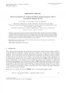
Table 1: Monte Carlo simulation comparison table: common random number method versus control variate method for Asian arithmetic option. 𝐾
𝑇
Estimated Delta of Asian arithmetic option by CRN method
Standard error by CRN method
Estimated Delta of Asian arithmetic option by control variate method
Standard error by control variate method
50
1 2 3
0.8682 0.8140 0.7795
0.1971 0.1909 0.1868
0.8806 0.8351 0.7783
0.0239 0.0240 0.0298
60
1 2 3
0.5630 0.5875 0.6030
0.1588 0.1622 0.1643
0.5687 0.5466 0.5969
0.0199 0.0380 0.0278
70
1 2 3
0.2405 0.3668 0.4228
0.1038 0.1282 0.1376
0.2514 0.3569 0.3492
0.0283 0.0311 0.0249
The table above is based on the Asian arithmetic option with the following parameters: 𝑆 = 60, 𝑟 = 0.05, sigma = 0.3, sample size 𝑛 = 5000, time step 𝑚 = 500, and initial stock price shock epsilon = 0.1.
Step 3 (finite difference approximation). Let 𝐶𝐴 (𝑆) be the Asian arithmetic option price under the Black-Scholes model, and then 𝜕𝐶𝐴 𝐶𝐴 (𝑆 + 𝜖) − 𝐶𝐴 (𝑆) ≈ 𝜕𝑆 𝜖 = 𝑒−𝑟𝑇
̃ 𝐴 (𝑆)) − E𝑄 (Φ𝐴 (𝑆)) E𝑄 (Φ 𝜖
𝑛 (1/𝑚) ∑𝑗=1 −𝑟𝑇
≈𝑒 =
̃ (𝑗) (𝑆) − (1/𝑚) ∑𝑛 Φ(𝑗) (𝑆) Φ 𝑗=1 𝐴 𝐴
(32)
𝜖
−𝑟𝑇 𝑛
𝑒 ̃ (𝑗) (𝑆) − Φ(𝑗) (𝑆)) =: Δ ̂ 𝐴. ∑ (Φ 𝐴 𝑚𝜖 𝑗=1 𝐴
Similarly, we construct the sample estimator for Asian geometric option price 𝐶𝐺(𝑆), 𝜕𝐶𝐺 𝑒−𝑟𝑇 𝑛 ̃ (𝑗) (𝑗) ̂ 𝐺. ≈ ∑ (Φ (𝑆) − Φ𝐺 (𝑆)) =: Δ 𝜕𝑆 𝑚𝜖 𝑗=1 𝐺
(33)
Step 4 (define the control sample estimator for Asian geometric option Greeks Δ). Consider ̂ Control = Δ ̂ 𝐴 − (Δ ̂ 𝐺 − Δ 𝐺) . Δ
(34)
Next, let us take a look at the results of our proposed numerical simulation and compare it with the classic Common Random Number (CRN for short) with Table 1. It is very clear that our proposed method is better than the CRN method in the sense that it introduce much smaller standard error than the classic CRN method with the same other parameters.
6. Conclusion We study the numerical solution for the Delta of Asian arithmetic option, which was known to have no explicit analytical
closed form solution. With the Delta of Asian geometric option as a control, we provided a simple, fast, intuitive, and reliable numerical solution in the sense that the standard errors of Monte Carlo simulation were reduced greatly. We also mention that, in recent years, many authors have been actively involved in the research of calculating Greeks of Asian type option using various approaches. For instance, in [13], the authors provided formulas for the Greeks of Asian arithmetic option, which involves the time integral of geometric Brownian motion. As stated in the paper, the results are consistent with the Monte Carlo simulation. In [14], with the advanced tool of Malliavin calculus, the authors give a quasiexplicit formula for the Asian option Greeks. Also, in [15], a PDE approach was utilized to understand the numerical value of the Asian option Greeks. To summarize, we believe that it is challenging but worth efforts to obtain more accurate value for the Asian arithmetic option Greeks, for the purpose of hedging strategy. Among various approximating methods, our numerical scheme provides a very neat and efficient choice when one wants to calculate hedge position of a portfolio that involves the Asian average options. Because the assumption of high correlation for the two variates needs to hold, the performance on other Greeks, however, still needs to be examined.
Conflict of Interests The authors declare that there is no conflict of interests regarding the publication of this paper.
Acknowledgments This research is supported by National Natural Science Foundation of China under Grants (nos. 71171035 and 71471030) and MOE (Ministry of Education in China) Youth Foundation Project of Humanities and Social Sciences (no. 13YJC790185).
6
References [1] W. Falloon and D. Turner, “The evolution of a market,” in Managing Energy Price Risk, Risk Books, London, UK, 1999. [2] S. M. Turnbull and L. M. Wakeman, “A quick algorithm for pricing European average options,” The Journal of Financial and Quantitative Analysis, vol. 26, no. 3, pp. 377–389, 1991. [3] T. Vorst, “Prices and hedge ratios of average exchange rate options,” International Review of Financial Analysis, vol. 1, no. 3, pp. 179–193, 1992. [4] E. Levy, “Pricing European average rate currency options,” Journal of International Money and Finance, vol. 11, no. 5, pp. 474– 491, 1992. [5] E. Levy and S. Turnbull, “Average inteligence,” Risk, vol. 5, pp. 53–59, 1992. [6] M. Broadie and P. Glasserman, “Estimating security price derivatives using simulation,” Management Science, vol. 42, no. 2, pp. 269–285, 1996. [7] A. G. Z. Kemna and A. C. F. Vorst, “A pricing method for options based on average asset values,” Journal of Banking and Finance, vol. 14, no. 1, pp. 113–129, 1990. [8] M. Broadie, P. Glasserman, and S. G. Kou, “Connecting discrete and continuous path-dependent options,” Finance and Stochastics, vol. 3, no. 1, pp. 55–82, 1999. [9] E. Fourni´e, J.-M. Lasry, J. Lebuchoux, and P.-L. Lions, “Applications of Malliavin calculus to MONte-Carlo methods in finance. II,” Finance and Stochastics, vol. 5, no. 2, pp. 201–236, 2001. [10] A. Kohatsu-Higa and M. Montero, “Malliavin calculus in finance,” in Handbook of Computational and Numerical Methods in Finance, pp. 111–174, Birkh¨auser, 2004. [11] P. Boyle and A. Potapchik, “Prices and sensitivities of Asian options: a survey,” Insurance: Mathematics & Economics, vol. 42, no. 1, pp. 189–211, 2008. [12] T. Bjork, Arbitrage Theory in Continuous Time, Oxford University Press, 2004. [13] J. Choi and K. Kim, “The derivatives of Asian call option prices,” Communications in Mathematical Sciences, vol. 6, no. 3, pp. 557– 568, 2008. [14] Z. Yang, C. O. Ewald, and O. Menkens, “Pricing and hedging of Asian options: quasi-explicit solutions via Malliavin calculus,” Mathematical Methods of Operations Research, vol. 74, no. 1, pp. 93–120, 2011. [15] Z. A. Elshegmani and R. R. Ahmed, “Analytical solution for an arithmetic asian option using Mellin transforms,” International Journal of Mathematical Analysis, vol. 5, no. 25–28, pp. 1259– 1265, 2011.
The Scientific World Journal