Hindawi Mathematical Problems in Engineering Volume 2018, Article ID 9454160, 8 pages https://doi.org/10.1155/2018/9454160
Research Article Optimal Control Based on the Polynomial Least Squares Method Constantin Bota , Bogdan C+runtu , M+d+lina Sofia Pas, ca, and Marioara L+p+dat Department of Mathematics “Politehnica” University of Timis, oara, P-ta Victoriei, 2, Timis, oara 300006, Romania Correspondence should be addressed to Constantin Bota;
[email protected] Received 23 August 2018; Accepted 17 October 2018; Published 28 October 2018 Guest Editor: Hiroaki Mukaidani Copyright © 2018 Constantin Bota et al. This is an open access article distributed under the Creative Commons Attribution License, which permits unrestricted use, distribution, and reproduction in any medium, provided the original work is properly cited. In this paper an approach for computing an optimal control law based on the Polynomial Least Squares Method (PLSM) is presented. The initial optimal control problem is reformulated as a variational problem whose corresponding Euler-Lagrange equation is solved by using PLSM. A couple of examples emphasize the accuracy of the method.
1. Introduction Optimal control problems occur in many areas of science and engineering such as system mechanics, hydrodynamics, elasticity theory, geometrical optics, and aerospace engineering, and they are one of the several applications and extensions of the calculus of variations. The beginning of optimal control is represented by the Brachistochrone problem formulated by Galileo in 1683: A mass material point m moves without friction along a vertical curve joining the points (𝑥0 , 𝑦0 ) and (𝑥1 , 𝑦1 ). There is the question of finding such a curve for which the scroll time is minimal, curve called brachistochrone. Galileo’s attempts to resolve it were incorrect [1, 2]. The problem raised great interest at that time and solutions were proposed by many mathematicians like Bernoulli, Leibnitz, l’Hopital, and Newton [1]. These results were published by Euler in 1744, who concluded “nothing at all takes place in the universe in which some rule of maximum or minimum does not appear.” Euler also formulated the problem in general terms as the problem of finding the curve 𝑦(𝑡) over the interval [𝑎, 𝑏] (with 𝑦(𝑎) and 𝑦(𝑏) known) which minimizes: 𝑏
𝐽 = ∫ 𝐹 (𝑡, 𝑦 (𝑡) , 𝑦 (𝑡)) 𝑑𝑡 𝑎
(1)
for some given function 𝐹(𝑡, 𝑦(𝑡), 𝑦 (𝑡)), where 𝑦 = 𝑑𝑦/𝑑𝑡. Euler presented a necessary condition of optimality for the curve 𝑦(𝑡): 𝑑 𝐹 (𝑡, 𝑦 (𝑡) , 𝑦 (𝑡)) = 𝐹𝑦 (𝑡, 𝑦 (𝑡) , 𝑦 (𝑡)) 𝑑𝑡 𝑦
(2)
where 𝐹𝑦 and 𝐹𝑦 represent the partial derivatives with respect to 𝑦 and 𝑦, respectively. The solution techniques proposed initially had been of a geometric nature until 1755 when Lagrange described an analytical approach, based on perturbations or “variations” of the optimal curve and using his “undetermined multipliers,” which led directly to Euler’s necessary condition, now known as the “Euler-Lagrange equation.” Euler also adopted this approach and renamed the subject “the calculus of variations” [3]. In the years to come, considerable efforts have been made to develop optimal control techniques. A classification of methods for solving optimal control problems is presented by Berkani et al. in [3]. Among the most used ones we mention the following. (i) The Dynamic Programming method, based on the principle of optimality, was first formulated by Bellman [4] and often used in the analysis and design of automatic control systems. Bellman’s partial differential equation and the boundary conditions included are necessary conditions for obtaining the minimum of the optimal control problem. (ii) The Pontryagin Minimum Principle [5] is built on defining the Hamiltonian function by introducing adjoint variables. The optimal control law is obtained by solving the canonical differential equations (the Hamilton equations) which are the necessary conditions of optimality according to the minimum principle [6]. The optimality conditions are in general not able to provide the exact optimum since the resulting two-point boundary value problem (Bellman partial differential equation) is not easy to be solved
2
Mathematical Problems in Engineering
analytically and usually computational methods are employed [7–9]. In this paper we apply the Polynomial Least Squares Method (PLSM) in order to compute approximate analytical polynomial solutions for a optimal control problems. This method was used by C. Bota and B. C˘aruntu in 2014 to compute approximate analytical solutions for the Brusselator system which is a fractional-order system of nonlinear differential equations [10]. In the following years the accuracy of the method is emphasized by its use in solving several types of differential equations [11–13]. The optimal control problem approached in this paper is the computation of the optimal control law 𝑢(𝑡) : [0, 𝑡𝑓 ] ⊂ R → R which minimizes the performance index: 𝑡𝑓
𝐽 = ∫ 𝐹 (𝑦 (𝑡) , 𝑢 (𝑡) , 𝑡) 𝑑𝑡 0
(3)
where the state equation is 𝑦 (𝑡) = 𝑓 (𝑦 (𝑡) , 𝑢 (𝑡) , 𝑡)
𝐽 = ∫ 𝐺 (𝑡, 𝑦 (𝑡) , 𝑦 (𝑡)) 𝑑𝑡 0
(5)
with 𝑦 (0) = 𝑦0 , 𝑦 (𝑡𝑓 ) = 𝑦𝑓
(6)
where the relation (5) is obtained from (3) by substituting the expression for 𝑢(𝑡) as a function of 𝑦(𝑡) (4). The necessary condition for the uniqueness of the solution to the problem (5)-(6) is that 𝑦(𝑡) satisfies the conditions (6) and the Euler-Lagrange equation: 𝜕𝐺 (𝑡, 𝑦 (𝑡) , 𝑦 (𝑡)) 𝜕𝑦 (𝑡)
𝑑 𝜕𝐺 (𝑡, 𝑦 (𝑡) , 𝑦 (𝑡)) = ( ). 𝑑𝑡 𝜕𝑦 (𝑡)
(7)
(9)
̃ an approximate solution of (8), the If we denote by 𝑦(𝑡) error obtained by replacing the exact solution 𝑦(𝑡) with the ̃ is given by the remainder: approximation 𝑦(𝑡) R (𝑡, 𝑦̃ (𝑡)) = 𝐷 (𝑦̃ (𝑡)) ,
𝑡 ∈ [0, 𝑡𝑓 ] .
(10)
Taking into account the boundary conditions (6), for 𝜖 ∈ 𝑅+, we will compute approximate polynomial solutions 𝑦̃ of the problem (8), (6) on the interval [0, 𝑡𝑓 ] as follows. Definition 1. We call an 𝜖-approximate polynomial solution of the problem (8), (6) an approximate polynomial solution 𝑦̃ satisfying the relations ̃ < 𝜖 (11) R (𝑡, 𝑦) 𝑦̃ (0) = 𝑦0 , 𝑦̃ (𝑡𝑓 ) = 𝑦𝑓
(12)
We call a weak 𝜖-approximate polynomial solution of the problem (8), (6) an approximate polynomial solution 𝑦̃ satisfying the relation 𝑡
𝑓 ̃ 𝑑𝑡 ≤ 𝜖 ∫ R (𝑡, 𝑦) 0
(13)
together with the initial conditions (6) Definition 2. Let 𝑃𝑚 (𝑡) = 𝑐0 + 𝑐1 𝑡 + 𝑐2 𝑡2 + ⋅ ⋅ ⋅ + 𝑐𝑚 𝑡𝑚 , 𝑐𝑖 ∈ R, 𝑖 = 0, 1, . . . , 𝑚, be a sequence of polynomials satisfying the conditions 𝑃𝑚 (0) = 𝑦0 , 𝑃𝑚 (𝑡𝑓 ) = 𝑦𝑓 . We call the sequence of polynomials 𝑃𝑚 (𝑡) convergent to the solution of the problem (8), (6) if lim𝑚→∞ 𝐷(𝑃𝑚 (𝑡)) = 0. We observe that from the hypothesis of the initial problem (8), (6) it follows that there exists a sequence of polynomials 𝑃𝑚 (𝑡) which converges to the solution of the problem. We will compute a weak 𝜖-approximate polynomial solution, in the sense of the Definition 1, of the type 𝑚
𝑦̃ (𝑡) = ∑ 𝑑𝑘 𝑡𝑘
(14)
𝑘=0
where 𝑑0 , 𝑑1 , . . . , 𝑑𝑚 are constants which are calculated using the following steps: (i) By substituting the approximate solution (14) in (8) we obtain the remainder:
2. Approximate Solution for an Optimal Control Problem Using the Polynomial Least Squares Method
̃ = 𝑦̃ (𝑡) − F (𝑦̃ (𝑡) , 𝑦̃ (𝑡) , 𝑡) R (𝑡, 𝑦)
2.1. The Polynomial Least Squares Method. The EulerLagrange equation associated with the optimal problem (5)(6) may have the expression: 𝑦 (𝑡) = F (𝑦 (𝑡) , 𝑦 (𝑡) , 𝑡)
𝐷 (𝑦 (𝑡)) = 𝑦 (𝑡) − F (𝑦 (𝑡) , 𝑦 (𝑡) , 𝑡)
(4)
and the state variable 𝑦(𝑡) satisfies the constraints 𝑦(0) = 𝑦0 and 𝑦(𝑡𝑓 ) = 𝑦𝑓 . We will assume that F is of class 𝐶1 , so the solution of the optimal control problem exists and is unique for the given conditions. The state equation (4) may be linear or nonlinear but we also assume that 𝑢(𝑡) can be explicitly obtained from (4) as a function of 𝑦(𝑡). In this case solving the optimal control problem is equivalent to solving the variational problem of finding the minimum of functional: 𝑡𝑓
where F may be linear or nonlinear. We associate with this equation the following operator:
(8)
(15)
We remark that if we could find 𝑑0 , 𝑑1 , . . . , 𝑑𝑚 such ̃ = 0, 𝑦(0) ̃ ̃ 𝑓 ) = 𝑦𝑓 , then that R(𝑡, 𝑦) = 𝑦0 , 𝑦(𝑡 by substituting 𝑑0 , 𝑑1 , . . . , 𝑑𝑚 in (14) we would obtain the exact solution of the problem (8), (6). This is not generally possible, unless the exact solution is actually a polynomial
Mathematical Problems in Engineering
3
(16)
2.2. Application of the Polynomial Least Squares Method for an Optimal Control Problem. We will find the approximate solution of the optimal control problem (3)-(4) using the following steps:
where 𝑑0 , 𝑑1 are computed as functions of 𝑑2 , 𝑑3 ⋅ ⋅ ⋅ 𝑑𝑚 using the conditions (6).
(i) We transform the optimal control problem (3)-(4) in a variational problem (5)-(6) as described in the introduction.
(ii) We attach to the problem (8), (6) the following functional: 𝑡𝑓
J (𝑑2 , 𝑑3 ⋅ ⋅ ⋅ , 𝑑𝑚 ) = ∫ R2 (𝑡, 𝑦̃ (𝑡)) 𝑑𝑡 0
(iii) We compute the values 𝑑02 , 𝑑03 , ⋅ ⋅ ⋅ 𝑑0𝑚 as the values which give the minimum of the functional J and the values of 𝑑00 and 𝑑01 as functions of 𝑑02 , 𝑑03 , ⋅ ⋅ ⋅ 𝑑0𝑚 using the conditions (6). (iv) Using the constants 𝑑02 , 𝑑03 , ⋅ ⋅ ⋅ 𝑑0𝑚 previously determined we compute the polynomial 𝑚
∑ 𝑑0𝑘 𝑡𝑘 𝑘=0
𝑀𝑚 (𝑡) =
(17)
Theorem 3. The sequence of polynomials 𝑀𝑚 (𝑡) from (17) satisfies the property
(ii) We attach to the variational problem (5)-(6) the corresponding Euler-Lagrange equation (7), (8). ̃ of the (iii) We compute the approximate solution 𝑦(𝑡) Euler-Lagrange equation using PLSM as described in ̃ is an approximation of the previous section. Thus 𝑦(𝑡) the state variable 𝑦(𝑡) of the optimal control problem. ̃ of the opti(iv) Finally we compute an approximation 𝑢(𝑡) mal control law 𝑢(𝑡) by means of the state equation (4).
3. Applications
(18)
In this section we apply the Polynomial Least Squares Method in order to compute analytical approximate optimal control laws for three optimal control problems.
Moreover, if ∀𝜖 > 0, ∃𝑚𝑜 ∈ N, 𝑚 > 𝑚0 , it follows that 𝑀𝑚 (𝑡) is a weak 𝜖-approximate polynomial solution of the problem (8), (6)
3.1. Application 1. We consider the following optimal control problem [3]:
𝑡𝑓
lim ∫ R2 (𝑡, 𝑀𝑚 (𝑡)) 𝑑𝑡 = 0
𝑡→∞ 0
Proof. Based on the way the polynomials 𝑀𝑚 (𝑡) are computed and taking into account the relations (15)-(17), the following inequalities are satisfied: 𝑡f
𝑡𝑓
0
0
0 ≤ ∫ R2 (𝑡, 𝑀𝑚 (𝑡)) 𝑑𝑡 ≤ ∫ R2 (𝑡, 𝑃𝑚 (𝑡)) 𝑑𝑡,
1
𝑢(𝑡)
1 𝑦 (𝑡) = 𝑢 (𝑡) − √𝑦 (𝑡) 4
𝑦 (0) = 0, 𝑦 (1) = 2
𝑡𝑓
0 ≤ lim ∫ R2 (𝑡, 𝑀𝑚 (𝑡)) 𝑑𝑡 𝑡𝑓
(20)
≤ lim ∫ R (𝑡, 𝑃𝑚 (𝑡)) 𝑑𝑡 = 0.
(24)
𝑦 (𝑡)
𝑡→∞ 0
=
We obtain 𝑏
(23)
The exact solution of this problem is [3]
2
lim ∫ R2 (𝑡, 𝑀𝑚 (𝑡)) 𝑑𝑡 = 0.
(22)
and the boundary conditions are
where 𝑃𝑚 (𝑡) is the sequence of polynomials introduced in Definition 2. It follows that 𝑡→∞ 0
0
where the state equation is
(19)
∀𝑚 ∈ N,
2
min ∫ [(2 − 𝑦 (𝑡)) + 𝑢2 (𝑡)] 𝑑𝑡
𝑒−𝑡 (−𝑒 − 63𝑒2 − 63𝑒𝑡 + 63𝑒2𝑡 + 63𝑒2+𝑡 + 𝑒1+2𝑡 )
(25)
32 (−1 + 𝑒2 )
(21)
In order to apply PLSM we follow the steps presented in the previous section:
From this limit we obtain that ∀𝜖 > 0, ∃𝑚𝑜 ∈ N, 𝑚 > 𝑚0 and it follows that 𝑀𝑚 (𝑡) is a weak 𝜖-approximate polynomial solution of the problem (8), (6).
(i) From the state equation (23) we obtain the optimal control law 𝑢(𝑡) as a function of the state variable 𝑦(𝑡):
𝑡→∞ 𝑎
Remark 4. In order to find 𝜖-approximate polynomial solutions of the problem (8), (6) by using the Polynomial Least Squares Method we will first determine weak approximate ̃ If |R(𝑡, 𝑦)| ̃ < 𝜖 then 𝑦̃ is also an 𝜖polynomial solutions, 𝑦. approximate polynomial solution of the problem.
1 𝑢 (𝑡) = 𝑦 (𝑡) + √𝑦 (𝑡) 4
(26)
Replacing this expression of 𝑢(𝑡) in the performance index (22) we transform the initial optimal control problem into the following variational problem:
4
Mathematical Problems in Engineering (a) Find the minimum of the functional 1 2 1 2 ∫ [(2 − 𝑦 (𝑡)) + (𝑦 (𝑡) + √𝑦 (𝑡)) (𝑡)] 𝑑𝑡 4 0
(27)
subject to the boundary conditions (24). (ii) The corresponding Euler-Lagrange equation is 𝑦 (𝑡) − 𝑦 (𝑡) +
63 =0 32
(28)
(iii) We compute using PLSM an approximate analytical solution of the type 𝑦̃ (𝑡) = 𝑑0 + 𝑑1 ⋅ 𝑡 + 𝑑2 ⋅ 𝑡2 + 𝑑3 ⋅ 𝑡3 + 𝑑4 ⋅ 𝑡4 + 𝑑5 ⋅ 𝑡5 + 𝑑6 ⋅ 𝑡6 + 𝑑7 ⋅ 𝑡7 + 𝑑8 ⋅ 𝑡8 + 𝑑9 ⋅ 𝑡9 .
(29)
From the boundary conditions (24) we obtain 𝑑̃0 = 0 and 𝑑1 = 2 − 𝑑2 − 𝑑3 − 𝑑4 − 𝑑5 − 𝑑6 − 𝑑7 − 𝑑8 − 𝑑9 . The corresponding remainder (15) is R (𝑡) = −
63 − 2 ⋅ (2 ⋅ 𝑑2 + 6 ⋅ 𝑑3 ⋅ 𝑡 + 12 ⋅ 𝑑4 ⋅ 𝑡2 + 20 16
(30)
⋅ 𝑡7 + 𝑑8 ⋅ 𝑡8 + 𝑑9 ⋅ 𝑡9 ) . By minimizing the functional (16) J(𝑑2 , 𝑑3 ⋅ ⋅ ⋅ , 𝑑9 ) (too large to be included here) we obtain the values for 𝑑2 , 𝑑3 ⋅ ⋅ ⋅ , 𝑑9 . We compute the corresponding values of 𝑑0 and 𝑑1 using again the conditions (24) and ̃ to obtain our we replace all these values in 𝑦(𝑡) approximation: 𝑦̃ (𝑡) = 2.6116294098342876 ⋅ 𝑡 + 0.9843749991096482 ⋅ 𝑡
+ 0.43527154661696676 ⋅ 𝑡3 + 0.08203105649571096 ⋅ 𝑡4
+ 0.0000454584242327247 ⋅ 𝑡8 + 0.000005327350329483319 ⋅ 𝑡9 .
2.×10−10 1.5×10⁻¹⁰
0.2
0.4
0.6
0.8
1.0
Figure 1: The absolute errors corresponding to the approximations ̃ in Application 1: approximate solution from of the state variable 𝑦(𝑡) [3] given by VIM (red curve) and approximate solution given by PLSM (blue curve).
(iv) Finally we can easily compute an approximation for 𝑢̃(𝑡) (also not included here because of its large size) by means of (26): 1 𝑢̃ (𝑡) = 𝑦̃ (𝑡) + √𝑦̃ (𝑡) 4
2
+ 0.0005146366961518619 ⋅ 𝑡7
𝑢̃(𝑡) 4.440892099 ⋅ 10−16 2.194910920 ⋅ 10−11 1.921662829 ⋅ 10−11 7.726264073 ⋅ 10−12 2.682920552 ⋅ 10−11 1.299405028 ⋅ 10−12 2.589484183 ⋅ 10−11 9.465761508 ⋅ 10−12 1.677147310 ⋅ 10−11 2.004618693 ⋅ 10−11 0
Error of y VIM Error of y PLSM
+ 𝑑2 ⋅ 𝑡2 + 𝑑3 ⋅ 𝑡3 + 𝑑4 ⋅ 𝑡4 + 𝑑5 ⋅ 𝑡5 + 𝑑6 ⋅ 𝑡6 + 𝑑7
+ 0.0027321111314777993 ⋅ 𝑡6
̃ 𝑦(𝑡) 0 2.317035452 ⋅ 10−13 6.393774399 ⋅ 10−13 1.423638984 ⋅ 10−12 7.804867863 ⋅ 10−14 1.620037438 ⋅ 10−12 2.264854970 ⋅ 10−13 1.334266031 ⋅ 10−12 6.727951529 ⋅ 10−13 1.718625242 ⋅ 10−13 2.220446049 ⋅ 10−16
5.×10−11
⋅ ((2 − 𝑑2 − 𝑑3 − 𝑑4 − 𝑑5 − 𝑑6 − 𝑑7 − 𝑑8 − 𝑑9 ) ⋅ 𝑡
+ 0.021762704663334236 ⋅ 𝑡5
𝑡 0 0.1 0.2 0.3 0.4 0.5 0.6 0.7 0.8 0.9 1.0
1.×10−10
⋅ 𝑑5 ⋅ 𝑡3 + 30 ⋅ 𝑑6 ⋅ 𝑡4 + 42 ⋅ 𝑑7 ⋅ 𝑡5 + 56 ⋅ 𝑑8 ⋅ 𝑡6 + 72 ⋅ 𝑑9 ⋅ 𝑡7 ) + 2
Table 1: Absolute errors of the approximations of the state variable ̃ and the optimal control law 𝑢̃(𝑡) obtained by using PLSM for 𝑦(𝑡) Application 1.
(31)
(32)
Table 1 presents the absolute errors (as differences in absolute value between the exact value and the approximate one) corresponding to our approximations of the state varĩ and of the optimal control law 𝑢(𝑡) ̃ obtained by using able 𝑦(𝑡) PLSM. Figures 1 and 2 present the comparison between our results and previous ones computed in [3] by using the Variational Iteration Method (VIM). It can be easily observed that not only is our approximation more precise, but while the error function corresponding to the VIM approximations shows a sizeable increase with 𝑡, the error function corresponding to PLSM does not. Moreover, another advantage of PLSM is the fact that, evidently, the approximation has the
Mathematical Problems in Engineering
5
2.5×10⁻¹⁰
2.×10−12
2.×10−10
1.5×10⁻¹²
1.5×10⁻¹⁰ 1.×10
1.×10−12
−10
5.×10−13
5.×10−11 0.2
0.4
0.6
0.8
1.0
Error of u VIM Error of u PLSM
simplest possible form, namely, a polynomial, and thus is very easy to use in any further computations. Finally, we mention ̃ the fact that by increasing the degree of the polynomial 𝑦(𝑡) we can obtain higher accuracy: for example, using a 10-th degree polynomial we obtain an overall error of 10−14 . 3.2. Application 2. Our second application is the optimal control problem: min ∫ 𝑢(𝑡)
0
2
1 + 𝑦 (𝑡) 𝑑𝑡 𝑢2 (𝑡)
(33)
𝑦 (𝑡) = 𝑢 (𝑡)
(34)
and the boundary conditions are 𝑦 (0) = 0, 𝑦 (1) = 0.5
(35)
(i) Replacing the expression of 𝑢(𝑡) from (34) in the performance index (33) we obtain the variational problem [6]: 1
𝑦(𝑡)
0
0.6
0.8
1.0
1 + 𝑦2 (𝑡) 𝑑𝑡 𝑦2 (𝑡)
(36)
with the same boundary conditions 𝑦(0) = 0, 𝑦(1) = 0.5. The exact solution of this problem is [6] 1 𝑦 (𝑡) = sinh (𝑡 ⋅ sinh−1 ( )) 2
Figure 3: The absolute error corresponding to the approximation of ̃ in Application 2: approximate solution given the state variable 𝑦(𝑡) by PLSM.
(ii) The corresponding nonlinear Euler Lagrange equation is 𝑦 (𝑡) (1 + 𝑦2 (𝑡)) − 𝑦 (𝑡) 𝑦 (𝑡) = 0
(38)
(iii) We compute using PLSM an approximate analytical solution of the type 𝑦̃ (𝑡) = 𝑑0 + 𝑑1 ⋅ 𝑡 + 𝑑2 ⋅ 𝑡2 + 𝑑3 ⋅ 𝑡3 + 𝑑4 ⋅ 𝑡4 + 𝑑5 ⋅ 𝑡5 + 𝑑6 ⋅ 𝑡6 + 𝑑7 ⋅ 𝑡7 .
(39)
From the boundary conditions (35) we obtain 𝑑̃0 = 0 and 𝑑1 = 1/2 − 𝑑2 − 𝑑3 − 𝑑4 − 𝑑5 − 𝑑6 − 𝑑7 .
where there state equation is
min ∫
0.4
Error of y PLSM
Figure 2: The absolute errors corresponding to the approximations of the optimal control law 𝑢̃(𝑡) in Application 1: approximate solution from [3] given by VIM (red curve) and approximate solution given by PLSM (blue curve).
1
0.2
(37)
We apply the same steps as in the previous application:
We compute again the corresponding reminder (15) and by minimizing the functional (16) J(𝑑2 , 𝑑3 ⋅ ⋅ ⋅ , 𝑑7 ) we obtain the values for 𝑑2 ⋅ ⋅ ⋅ 𝑑7 . Using the ̃ our conditions (35) and replacing all the values in 𝑦, approximation of the state variable is 𝑦̃ = 0.4812118250596084 ⋅ 𝑡 − 5.310800720418878 ⋅ 10−10 ⋅ 𝑡2 + 0.018571962082159076 ⋅ 𝑡3 − 3.347040175284603 ⋅ 10−8 ⋅ 𝑡4 + 0.00021510474426296038 ⋅ 𝑡5
(40)
− 8.131321771683893 ⋅ 10−8 ⋅ 𝑡6 + 1.2234286690670117 ⋅ 10−6 ⋅ 𝑡7 (iv) Using the state equation (34) we compute an approximation for the optimal control law 𝑢̃(𝑡). In Figures 3 and 4 we present the absolute errors cor̃ responding to our approximations of the state variable 𝑦(𝑡) and of the optimal control law 𝑢̃(𝑡) for the problem (33)-(35) obtained by using PLSM.
6
Mathematical Problems in Engineering Approximate solutions for this problem were proposed in [14] using the Homotopy Analysis Method and in [15] using the Optimal Homotopy Analysis Method. The exact solution of the problem is 𝑦 (𝑡) =
𝑒−2𝑡 ((5 + 45𝑒2 + 72𝑒4 ) 𝑒4𝑡 + 𝑒2 (−40 − 45𝑒2 + 27𝑒4 )) (47) (1 + 𝑒2 ) (9𝑒4 − 5)
The corresponding expression of the control is 𝑢 (𝑡) Figure 4: The absolute error corresponding to the approximation of the optimal control law 𝑢̃(𝑡) in Application 2: approximate solution given by PLSM.
3.3. Application 3. Our third application is the well-known linear quadratic regulator (LQR), more precisely the finitehorizon, continuous-time LQR. LQRs have a wide range of applications in engineering such as trajectory tracking and optimization in robotics, control system design for various types of vehicles, automatic voltage regulators in electrical generators, and optimal controls for various types of motors. The corresponding optimal control problem may be formulated as 𝐽=
𝑇 1 𝑥 (𝑡𝑓 ) 𝑆𝑥 (𝑡𝑓 ) 2
=
𝑒−2𝑡 ((5 + 45𝑒2 + 72𝑒4 ) 𝑒4𝑡 + 3𝑒2 (40 + 45𝑒2 − 27𝑒4 )) (48) (1 + 𝑒2 ) (9𝑒4 − 5)
Using the same steps presented in the previous examples we computed the following approximation of the state variable: 𝑦̃ (𝑡) = 3.041119828603783 − 1.8976676950657474 ⋅ 𝑡 + 6.08223965125759 ⋅ 𝑡2 − 1.2651116099552036 ⋅ 𝑡3 + 2.027411010322069 ⋅ 𝑡4 − 0.2530087549866359 ⋅ 𝑡5 + 0.2702720790557366 ⋅ 𝑡6
1 𝑡𝑓 + ∫ (𝑥𝑇 𝑃𝑥 + 2𝑥𝑇 𝑄𝑢 + 𝑢𝑇𝑅𝑢) 𝑑𝑡 2 𝑡0
𝑥 (𝑡) = 𝐴𝑥 (𝑡) + 𝐵𝑢 (𝑡)
(41)
− 0.02398312502575098
(49)
⋅ 𝑡7 0.01913989850290996 ⋅ 𝑡8 (42)
𝑥 (𝑡0 ) = 𝑥0 ,
− 0.0011806615481455588 ⋅ 𝑡9 + 0.0007696532612724977 ⋅ 𝑡10
𝑥 (𝑡𝑓 ) = 𝑥𝑓 ,
(43) 𝑡 ∈ [𝑡0 , 𝑡𝑓 ] .
+ 0.000022587123028528187 ⋅ 𝑡12 .
We consider the following particular case of the problem (41)-(43) corresponding to the values A=1, B=1, S=8, P=3, Q=0, R=1, and 𝑡𝑓 =1 [14, 15]: The performance index is 𝐽 = 4 ⋅ 𝑦2 (1) +
1 1 ∫ (3 ⋅ 𝑦2 (𝑡) + 𝑢2 (𝑡)) 𝑑𝑡 2 0
(44)
the state equation is 𝑦 (𝑡) = 𝑢 (𝑡)
(45)
and the boundary conditions are 𝑦 (0) = 3 + 𝑦 (1) = 8
20 , 9𝑒4 − 5
− 0.00002286154490479068 ⋅ 𝑡11
In Figures 5 and 6 we present the absolute errors cor̃ responding to our approximations of the state variable 𝑦(𝑡) and of the optimal control law 𝑢̃(𝑡) for the problem (44)-(46) obtained by using PLSM. The accuracy of our method is emphasized by a comparison with approximate solutions for Application 3 previously computed by means of other well-known methods. Table 2 presents a comparison of the absolute errors corresponding ̃ obtained to the approximations of the state variable 𝑦(𝑡) by using the Homotopy Analysis Method (HAM [14]) and by using the Optimal Homotopy Analysis Method (OHAM [15]).
4. Conclusion (46)
In this paper the application of the Polynomial Least Squares Method to optimal control problems is presented.
Mathematical Problems in Engineering
7
̃ obtained by using HAM, OHAM, Table 2: Comparison of the absolute errors corresponding to the approximations of the state variable 𝑦(𝑡) and PLSM for Application 3. ̃ 𝑂𝐻𝐴𝑀 𝑦(𝑡) 2.2926 ⋅ 10−7 8.7067 ⋅ 10−7 3.1004 ⋅ 10−7 6.0923 ⋅ 10−8 7.4523 ⋅ 10−9 3.7303 ⋅ 10−14
̃ 𝐻𝐴𝑀 𝑦(𝑡) 3.8034 ⋅ 10−4 3.7677 ⋅ 10−4 1.2227 ⋅ 10−4 1.5453 ⋅ 10−4 2.1309 ⋅ 10−4 0
𝑡 0 0.2 0.4 0.6 0.8 1.0
̃ 𝑃𝐿𝑆𝑀 𝑦(𝑡) 4.4409 ⋅ 10−16 1.7306 ⋅ 10−12 3.8681 ⋅ 10−12 9.6811 ⋅ 10−13 1.6227 ⋅ 10−12 0
The numerical examples included clearly illustrate the accuracy of the method by means of a comparison with solutions previously computed by other methods.
4.×10−12 3.×10−12
Data Availability 2.×10−12
The data used to support the findings of this study are included within the article.
1.×10−12
Conflicts of Interest 0.2
0.4
0.6
0.8
1.0
Error of y PLSM
Figure 5: The absolute error corresponding to the approximation of ̃ in Application 3: approximate solution given the state variable 𝑦(𝑡) by PLSM.
Figure 6: The absolute error corresponding to the approximation of the optimal control law 𝑢̃(𝑡) in Application 3: approximate solution given by PLSM.
In order to apply PLSM the optimal problem is transformed to a variational problem by substituting in the performance index the expression of the control variable given by the state equation. PLSM is able to find accurate approximations of the state variable by computing approximate analytical polynomial solutions of the Euler-Lagrange equation corresponding to the variational problem. The optimal control law is then computed by using the state equation.
The authors declare that they have no conflicts of interest.
References [1] R. W. Sargent, “Optimal control,” Journal of Computational and Applied Mathematics, vol. 124, no. 1-2, pp. 361–371, 2000. [2] H. J. Sussmann and J. C. Willems, “300 years of optimal control: from the brachystochrone to the maximum principle,” IEEE Control Systems Magazine, vol. 17, no. 3, pp. 32–44, 1997. [3] S. Berkani, F. Manseur, and A. Maidi, “Optimal control based on the variational iteration method,” Computers & Mathematics with Applications. An International Journal, vol. 64, no. 4, pp. 604–610, 2012. [4] R. Luus, “On the application of iterative dynamic programming to singular optimal control problems,” Institute of Electrical and Electronics Engineers Transactions on Automatic Control, vol. 37, no. 11, pp. 1802–1806, 1992. [5] M. J. Sewell, Maximum and Minimum Principles. A Unified Approach, with Applications, Cambridge University Press, New York, NY, USA, 1987. [6] M. Tatari and M. Dehghan, “Solution of problems in calculus of variations via He’s variational iteration method,” Physics Letters A, vol. 362, no. 5-6, pp. 401–406, 2007. [7] B. van Brunt, The Calculus of Variations, Springer, New York, NY, USA, 2004. [8] J.-H. He, “Variational iteration method for autonomous ordinary differential systems,” Applied Mathematics and Computation, vol. 114, no. 2-3, pp. 115–123, 2000. [9] I. Kucuk, “Active Optimal Control of the KdV Equation Using the Variational Iteration Method,” Mathematical Problems in Engineering, vol. 2010, Article ID 929103, 10 pages, 2010. [10] C. Bota and B. C˘aruntu, “Approximate Analytical Solutions of the Fractional-Order Brusselator System Using the Polynomial Least Squares Method,” Advances in Mathematical Physics, vol. 2015, Article ID 450235, 5 pages, 2015. [11] C. Bota and B. Caruntu, “Analytic approximate solutions for a class of variable order fractional differential equations using
8
[12]
[13]
[14]
[15]
Mathematical Problems in Engineering the polynomial least squares method,” Fractional Calculus and Applied Analysis, vol. 20, no. 4, pp. 1043–1050, 2017. C. Bota and B. Caruntu, “Analytical approximate solutions for quadratic Riccati differential equation of fractional order using the polynomial least squares method,” Chaos, Solitons & Fractals, vol. 102, pp. 339–345, 2017. B. Caruntu and C. Bota, “Approximate Analytical Solutions of the Regularized Long Wave Equation Using the Optimal Homotopy Perturbation Method,” The Scientific World Journal, vol. 201, Article ID 721865, 6 pages, 2014. M. S. Zahedi and H. S. Nik, “On homotopy analysis method applied to linear optimal control problems,” Applied Mathematical Modelling: Simulation and Computation for Engineering and Environmental Systems, vol. 37, no. 23, pp. 9617–9629, 2013. W. Jia, X. He, and L. Guo, “The optimal homotopy analysis method for solving linear optimal control problems,” Applied Mathematical Modelling: Simulation and Computation for Engineering and Environmental Systems, vol. 45, pp. 865–880, 2017.
Advances in
Operations Research Hindawi www.hindawi.com
Volume 2018
Advances in
Decision Sciences Hindawi www.hindawi.com
Volume 2018
Journal of
Applied Mathematics Hindawi www.hindawi.com
Volume 2018
The Scientific World Journal Hindawi Publishing Corporation http://www.hindawi.com www.hindawi.com
Volume 2018 2013
Journal of
Probability and Statistics Hindawi www.hindawi.com
Volume 2018
International Journal of Mathematics and Mathematical Sciences
Journal of
Optimization Hindawi www.hindawi.com
Hindawi www.hindawi.com
Volume 2018
Volume 2018
Submit your manuscripts at www.hindawi.com International Journal of
Engineering Mathematics Hindawi www.hindawi.com
International Journal of
Analysis
Journal of
Complex Analysis Hindawi www.hindawi.com
Volume 2018
International Journal of
Stochastic Analysis Hindawi www.hindawi.com
Hindawi www.hindawi.com
Volume 2018
Volume 2018
Advances in
Numerical Analysis Hindawi www.hindawi.com
Volume 2018
Journal of
Hindawi www.hindawi.com
Volume 2018
Journal of
Mathematics Hindawi www.hindawi.com
Mathematical Problems in Engineering
Function Spaces Volume 2018
Hindawi www.hindawi.com
Volume 2018
International Journal of
Differential Equations Hindawi www.hindawi.com
Volume 2018
Abstract and Applied Analysis Hindawi www.hindawi.com
Volume 2018
Discrete Dynamics in Nature and Society Hindawi www.hindawi.com
Volume 2018
Advances in
Mathematical Physics Volume 2018
Hindawi www.hindawi.com
Volume 2018