Research Article Parametric Rough Sets with

Hindawi Publishing Corporation Mathematical Problems in Engineering Volume 2013, Article ID 461363, 13 pages http://dx.doi.org/10.1155/2013/461363

Research Article Parametric Rough Sets with Application to Granular Association Rule Mining Xu He,1 Fan Min,1,2 and William Zhu1 1 2

Lab of Granular Computing, Minnan Normal University, Zhangzhou 363000, China School of Computer Science, Southwest Petroleum University, Chengdu 610500, China

Correspondence should be addressed to Fan Min; [email protected] Received 2 August 2013; Accepted 12 October 2013 Academic Editor: Gerhard-Wilhelm Weber Copyright © 2013 Xu He et al. This is an open access article distributed under the Creative Commons Attribution License, which permits unrestricted use, distribution, and reproduction in any medium, provided the original work is properly cited. Granular association rules reveal patterns hidden in many-to-many relationships which are common in relational databases. In recommender systems, these rules are appropriate for cold-start recommendation, where a customer or a product has just entered the system. An example of such rules might be “40% men like at least 30% kinds of alcohol; 45% customers are men and 6% products are alcohol.” Mining such rules is a challenging problem due to pattern explosion. In this paper, we build a new type of parametric rough sets on two universes and propose an efficient rule mining algorithm based on the new model. Specifically, the model is deliberately defined such that the parameter corresponds to one threshold of rules. The algorithm benefits from the lower approximation operator in the new model. Experiments on two real-world data sets show that the new algorithm is significantly faster than an existing algorithm, and the performance of recommender systems is stable.

1. Introduction Relational data mining approaches [1–4] look for patterns that include multiple tables in the database. These works generate rules through two measures, namely, support and confidence. Granular association rule mining [5, 6], combined with the granules [7–14], is a new approach to look for patterns hidden in many-to-many relationships. This approach generates rules with four measures to reveal connections between granules in two universes. A complete example of granular association rules might be “40% men like at least 30% kinds of alcohol; 45% customers are men and 6% products are alcohol.” Here 45%, 6%, 40%, and 30% are the source coverage, the target coverage, the source confidence, and the target confidence, respectively. With these four measures, the strength of the rule is well defined. Therefore, granular association rules are semantically richer than other relational association rules. Granular association rules [5, 6] are appropriate to solve the cold-start problem for recommender systems [15, 16]. Recommender systems [17–20] suggest products of interest to customers; therefore, they have gained much

success in E-commerce and similar applications. The coldstart problem [15, 16] is difficult in recommender systems. Recently, researchers have addressed the cold-start problem where either the customer or the product is new. Naturally, content-based filtering approaches [17, 21] are used for these problems. However, the situation with both new customer and new product has seldom been considered. A cold-start recommendation approach has been proposed based on granular association rules for the new situation. First, both customers and products are described through a number of attributes, thus forming different granules [8, 10, 22–24]. Then we generate rules between customers and products through satisfying four measures of granular association rules. Examples of granular association rules include “men like alcohol” and “Chinese men like France alcohol.” They are proposed at different degrees of granularity. Finally, we match the suitable rules to recommend products to customers. A granular association rule mining problem is defined as finding all granular association rules given thresholds on four measures [5]. Similar to other relational association rule mining problems (see, e.g., [25–27]), this problem is challenging due to pattern explosion. A straightforward

2 sandwich algorithm has been proposed in [5]. It starts from both entities and proceeds to the relation. Unfortunately, the time complexity is rather high and the performance is not satisfactory. In this paper, we propose a new type of parametric rough sets on two universes to study the granular association rule mining problem. We borrow some ideas from variable precision rough sets [28] and rough sets on two universes [29–31] to build the new model. The model is deliberately adjusted such that the parameter coincides with the target confidence threshold of rules. In this way, the parameter is semantic and can be specified by the user directly. We compare our definitions with alternative ones and point out that they should be employed in different applications. Naturally, our definition is appropriate for cold-start recommendation. We also study some properties, especially the monotonicity of the lower approximation, of our new model. With the lower approximation of the proposed parametric rough sets, we design a backward algorithm for rule mining. This algorithm starts from the second universe and proceeds to the first one; hence it is called a backward algorithm. Compared with an existing sandwich algorithm [5], the backward algorithm avoids some redundant computation. Consequently, it has a lower time complexity. Experiments are undertaken on two real-world data sets. One is the course selection data from Minnan Normal University during the semester between 2011 and 2012. The other is the publicly available MovieLens data set. Results show that (1) the backward algorithm is more than 2 times faster than the sandwich algorithm; (2) the run time is linear with respect to the data set size; (3) sampling might be a good choice to decrease the run time; and (4) the performance of recommendation is stable. The rest of the paper is organized as follows. Section 2 reviews granular association rules through some examples. The rule mining problem is also defined. Section 3 presents a new model of parametric rough sets on two universes. The model is defined to cope with the formalization of granular association rules. Then Section 4 presents a backward algorithm for the problem. Experiments on two real-world data sets are discussed in Section 5. Finally, Section 6 presents some concluding remarks and further research directions.

2. Preliminaries In this section, we revisit granular association rules [6]. We discuss the data model, the definition, and four measures of such rules. A rule mining problem will also be represented. 2.1. The Data Model. The data model is based on information systems and binary relations. Definition 1. 𝑆 = (𝑈, 𝐴) is an information system, where 𝑈 = {𝑥1 , 𝑥2 , . . . , 𝑥𝑛 } is the set of all objects, 𝐴 = {𝑎1 , 𝑎2 , . . . , 𝑎𝑚 } is the set of all attributes, and 𝑎𝑗 (𝑥𝑖 ) is the value of 𝑥𝑖 on attribute 𝑎𝑗 for 𝑖 ∈ {1, 2, . . . , 𝑛} and 𝑗 ∈ {1, 2, . . . , 𝑚}. An example of information system is given by Table 1(a), where 𝑈 = {𝑐1, 𝑐2, 𝑐3, 𝑐4, 𝑐5} and 𝐴 = {Age, Gender, Married,

Mathematical Problems in Engineering Country, Income, NumCars}. Another example is given by Table 1(b). In an information system, any 𝐴󸀠 ⊆ 𝐴 induces an equivalence relation [32, 33] 𝐸𝐴󸀠 = {(𝑥, 𝑦) ∈ 𝑈 × 𝑈 | ∀𝑎 ∈ 𝐴󸀠 , 𝑎 (𝑥) = 𝑎 (𝑦)}

(1)

and partitions 𝑈 into a number of disjoint subsets called blocks or granules. The block containing 𝑥 ∈ 𝑈 is 𝐸𝐴󸀠 (𝑥) = {𝑦 ∈ 𝑈 | ∀𝑎 ∈ 𝐴󸀠 , 𝑎 (𝑦) = 𝑎 (𝑥)} .

(2)

The following definition was employed by Yao and Deng [23]. Definition 2. A granule is a triple [23] 𝐺 = (𝑔, 𝑖 (𝑔) , 𝑒 (𝑔)) ,

(3)

where 𝑔 is the name assigned to the granule, 𝑖(𝑔) is a representation of the granule, and 𝑒(𝑔) is a set of objects that are instances of the granule. 𝑔 = 𝑔(𝐴󸀠 , 𝑥) is a natural name to the granule. The representation of 𝑔(𝐴󸀠 , 𝑥) is 𝑖 (𝑔 (𝐴󸀠 , 𝑥)) = ⋀ ⟨𝑎 : 𝑎 (𝑥)⟩ . 𝑎∈𝐴󸀠

(4)

The set of objects that are instances of 𝑔(𝐴󸀠 , 𝑥) is 𝑒 (𝑔 (𝐴󸀠 , 𝑥)) = 𝐸𝐴󸀠 (𝑥) .

(5)

The support of the granule is the size of 𝑒(𝑔) divided by the size of the universe, namely, supp (𝑔 (𝐴󸀠 , 𝑥)) = supp ( ⋀ ⟨𝑎 : 𝑎 (𝑥)⟩) 𝑎∈𝐴󸀠

󵄨 󵄨󵄨 󵄨𝐸 󸀠 (𝑥)󵄨󵄨󵄨 = supp (𝐸𝐴󸀠 (𝑥)) = 󵄨 𝐴 . |𝑈|

(6)

Definition 3. Let 𝑈 = {𝑥1 , 𝑥2 , . . . , 𝑥𝑛 } and 𝑉 = {𝑦1 , 𝑦2 , . . . , 𝑦𝑘 } be two sets of objects. Any 𝑅 ⊆ 𝑈×𝑉 is a binary relation from 𝑈 to 𝑉. The neighborhood of 𝑥 ∈ 𝑈 is 𝑅 (𝑥) = {𝑦 ∈ 𝑉 | (𝑥, 𝑦) ∈ 𝑅} .

(7)

When 𝑈 = 𝑉 and 𝑅 is an equivalence relation, 𝑅(𝑥) is the equivalence class containing 𝑥. From this definition we know immediately that, for 𝑦 ∈ 𝑉, 𝑅−1 (𝑦) = {𝑥 ∈ 𝑈 | (𝑥, 𝑦) ∈ 𝑅} .

(8)

A binary relation is more often stored in the database as a table with two foreign keys. In this way the storage is saved. For the convenience of illustration, here we represented it with an 𝑛 × 𝑘 Boolean matrix. An example is given in Table 1(c), where 𝑈 is the set of customers as indicated in Table 1(a) and 𝑉 is the set of products as indicated in Table 1(b). With Definitions 1 and 3, we propose the following definition.

Mathematical Problems in Engineering

3

Table 1: A many-to-many entity-relationship system. (a) Customer

CID 𝑐1 𝑐2 𝑐3 𝑐4 𝑐5

Name Ron Michelle Shun Yamago Wang

Age 20–29 20–29 20–29 30–39 30–39

Gender Male Female Male Female Male

Married No Yes No Yes Yes

Country USA USA China Japan China

Income 60 k–69 k 80 k–89 k 40 k–49 k 80 k–89 k 90 k–99 k

NumCars 0-1 0-1 0-1 2 2

(b) Product

PID 𝑝1 𝑝2 𝑝3 𝑝4 𝑝5 𝑝6

Name Bread Diaper Pork Beef Beer Wine

Country Australia China China Australia France France

Category Staple Daily Meat Meat Alcohol Alcohol

Color Black White Red Red Black White

Price 1–9 1–9 1–9 10–19 10–19 10–19

(c) Buys

𝑝1 1 1 0 0 1

CID\PID 𝑐1 𝑐2 𝑐3 𝑐4 𝑐5

𝑝2 1 0 1 1 0

𝑝3 0 0 0 0 0

Definition 4. A many-to-many entity-relationship system (MMER) is a 5-tuple ES = (𝑈, 𝐴, 𝑉, 𝐵, 𝑅), where (𝑈, 𝐴) and (𝑉, 𝐵) are two information systems and 𝑅 ⊆ 𝑈 × 𝑉 is a binary relation from 𝑈 to 𝑉. An example of MMER is given in Tables 1(a), 1(b), and 1(c). 2.2. Granular Association Rules with Four Measures. Now we come to the central definition of granular association rules. Definition 5. A granular association rule is an implication of the form (GR) : ⋀ ⟨𝑎 : 𝑎 (𝑥)⟩ 󳨐⇒ ⋀ ⟨𝑏 : 𝑏 (𝑦)⟩ , 𝑎∈𝐴󸀠

𝑏∈𝐵󸀠

(9)

where 𝐴󸀠 ⊆ 𝐴 and 𝐵󸀠 ⊆ 𝐵. According to (6), the set of objects meeting the left-hand side of the granular association rule is LH (GR) = 𝐸𝐴󸀠 (𝑥) ,

(10)

while the set of objects meeting the right-hand side of the granular association rule is RH (GR) = 𝐸𝐵󸀠 (𝑦) .

(11)

From the MMER given in Tables 1(a), 1(b), and 1(c), we may obtain the following rule.

𝑝4 1 1 0 1 1

𝑝5 1 0 1 1 1

𝑝6 0 1 1 0 1

Rule 1. One has ⟨Gender: Male⟩ 󳨐⇒ ⟨Category: Alcohol⟩ .

(12)

Rule 1 can be read as “men like alcohol.” There are some issues concerning the strength of the rule. For example, we may ask the following questions on Rule 1. (1) How many customers are men? (2) How many products are alcohol? (3) Do all men like alcohol? (4) Do all kinds of alcohol favor men? An example of complete granular association rules with measures specified is “40% men like at least 30% kinds of alcohol; 45% customers are men and 6% products are alcohol.” Here 45%, 6%, 40%, and 30% are the source coverage, the target coverage, the source confidence, and the target confidence, respectively. These measures are defined as follows. The source coverage of a granular association rule is scov (GR) =

|LH (GR)| . |𝑈|

(13)

The target coverage of GR is tcov (GR) =

|RH (GR)| . |𝑉|

(14)

4

Mathematical Problems in Engineering

There is a tradeoff between the source confidence and the target confidence of a rule. Consequently, neither value can be obtained directly from the rule. To compute any one of them, we should specify the threshold of the other. Let tc be the target confidence threshold. The source confidence of the rule is sconf (GR, tc) =

|{𝑥 ∈ LH (GR) | |𝑅 (𝑥) ∩ RH (GR)| / |RH (GR)| ≥ tc}| . |LH (GR)| (15) Let sc be the source confidence threshold, and |{𝑥 ∈ LH (GR) | |𝑅 (𝑥) ∩ RH (GR)| ≥ 𝐾 + 1}| < sc × |LH (GR)|

(16)

≤ |{𝑥 ∈ LH (GR) | |𝑅 (𝑥) ∩ RH (GR)| ≥ 𝐾}| . This equation means that sc×100% elements in LH(GR) have connections with at least 𝐾 elements in RH(GR), but less than sc × 100% elements in LH(GR) have connections with at least 𝐾 + 1 elements in RH(GR). The target confidence of the rule is tconf (GR, sc) =

𝐾 . |RH (GR)|

(17)

In fact, the computation of 𝐾 is nontrivial. First, for any 𝑥 ∈ LH(GR), we need to compute tc(𝑥) = |𝑅(𝑥) ∩ RH(GR)| and obtain an array of integers. Second, we sort the array in a descending order. Third, let 𝑘 = ⌊sc × | LH(GR)|⌋; 𝐾 is the kth element in the array. The relationships between rules are interesting to us. As an example, let us consider the following rule. Rule 2. One has ⟨Gender: Male⟩ ∧ ⟨Country: China⟩ 󳨐⇒ ⟨Category: Alcohol⟩ ∧ ⟨Country: France⟩ .

(18)

Rule 2 can be read as “Chinese men like France alcohol.” One may say that we can infer Rule 2 from Rule 1 since the former one has a finer granule. However, with the four measures we know that the relationships between these two rules are not so simple. A detailed explanation of Rule 2 might be “60% Chinese men like at least 50% kinds of France alcohol; 15% customers are Chinese men and 2% products are France alcohol.” Comparing Rules 1 and 2 is stronger in terms of source/target confidence; however it is weaker in terms of source/target coverage. Therefore if we need rules covering more people and products, we prefer Rule 1; if we need more confidence on the rules, we prefer Rule 2. For example, if the source confidence threshold is 55%, Rule 2 might be valid while Rule 1 is not; if the source coverage is 20%, Rule 1 might be valid while Rule 2 is not. 2.3. The Granular Association Rule Mining Problem. A straightforward rule mining problem is as follows.

Input. An ES = (𝑈, 𝐴, 𝑉, 𝐵, 𝑅), a minimal source coverage threshold ms, a minimal target coverage threshold mt, a minimal source confidence threshold sc, and a minimal target confidence threshold tc. Output. All granular association rules satisfying scov(GR) ≥ ms, tcov(GR) ≥ mt, sconf(GR) ≥ sc, and tconf(GR) ≥ tc. Since both sc and tc are specified, we can choose either (15) or (17) to decide whether or not a rule satisfies these thresholds. Equation (15) is a better choice.

3. Parametric Rough Sets on Two Universes In this section, we first review rough approximations [32] on one universe. Then we present rough approximations on two universes. Finally we present parametric rough approximations on two universes. Some concepts are dedicated to granular association rules. We will explain in detail the way they are defined from semantic point of view. 3.1. Classical Rough Sets. The classical rough sets [32, 34] are built upon lower and upper approximations on one universe. We adopt the ideas and notions introduced in [35] and define these concepts as follows. Definition 6. Let 𝑈 be a universe and 𝑅 ⊆ 𝑈 × 𝑈 an indiscernibility relation. The lower and upper approximations of 𝑋 ⊆ 𝑈 with respect to 𝑅 are 𝑅 (𝑋) = {𝑥 ∈ 𝑋 | 𝑅 (𝑥) ⊆ 𝑋} ,

(19)

𝑅 (𝑋) = {𝑥 ∈ 𝑋 | 𝑅 (𝑥) ∩ 𝑋 ≠ 0} ,

(20)

respectively. These concepts can be employed for set approximation or classification analysis. For set approximation, the interval [𝑅(𝑋), 𝑅(𝑋)] is called rough set of 𝑋, which provides an approximate characterization of 𝑋 by the objects that share the same description of its members [35]. For classification analysis, the lower approximation operator helps finding certain rules, while the upper approximation helps finding possible rules. 3.2. Existing Parametric Rough Sets. Ziarko [28] pointed out that the classical rough sets cannot handle classification with a controlled degree of uncertainty or a misclassification error. Consequently, he proposed variable precision rough sets [28] with a parameter to indicate the admissible classification error. Let 𝑋 and 𝑌 be nonempty subsets of a finite universe 𝑈, and 𝑌 ⊆ 𝑋. The measure 𝑐(𝑋, 𝑌) of the relative degree of misclassification of the set 𝑋 with respect to set 𝑌 is defined as {1 − 𝑐 (𝑋, 𝑌) = { {0,

|𝑋 ∩ 𝑌| , |𝑋| > 0, |𝑋| |𝑋| = 0,

where | ⋅ | denotes set cardinality.

(21)

Mathematical Problems in Engineering

5

The equivalence relation 𝑅 corresponds to a partitioning of 𝑈 into a collection of equivalence classes or elementary sets 𝑅∗ = {𝐸1 , 𝐸2 , . . . , 𝐸𝑛 }. The 𝛼-lower and 𝛼-upper approximation of the set 𝑈 ⊇ 𝑋 are defined as 𝑅𝛼 (𝑋) = ⋃ {𝐸 ∈ 𝑅∗ | 𝑐 (𝐸, 𝑋) ≤ 𝛼} , 𝑅𝛼 (𝑋) = ⋃ {𝐸 ∈ 𝑅∗ | 𝑐 (𝐸, 𝑋) < 1 − 𝛼} ,

(22)

where 0 ≤ 𝛼 < 0.5. For the convenience of discussion, we rewrite his definition as follows. Definition 7. Let 𝑈 be a universe and 𝑅 ⊆ 𝑈 × 𝑈 an indiscernibility relation. The lower and upper approximations of 𝑋 ⊆ 𝑈 with respect to 𝑅 under precision 𝛽 are |𝑅 (𝑥) ∩ 𝑋| ≥ 𝛽} , 𝑅𝛽 (𝑋) = {𝑥 ∈ 𝑈 | |𝑅 (𝑥)| 𝑅𝛽 (𝑋) = {𝑥 ∈ 𝑈 |

|𝑅 (𝑥) ∩ 𝑋| > 1 − 𝛽} , |𝑅 (𝑥)|

(23)

respectively. 𝑅(𝑥) is the equivalence class containing 𝑥. Note that 0.5 < 𝛽 ≤ 1 indicate the classification accuracy (precision) threshold rather than the misclassification error threshold as employed in [28]. Wong et al. [31] extended the definition to an arbitrary binary relation which is at least serial. Ziarko [28] introduced variable precision rough sets with a parameter. The model had seldom explanation about the parameter. Yao and Wong [36] studied the condition of parameter and introduced the decision theoretic rough set (DTRS) model. DTRS model is a probabilistic rough sets in the framework of Bayesian decision theory. It requires a pair of thresholds (𝛼, 𝛽) instead of only one in variable precision rough sets. Its main advantage is the solid foundation based on Bayesian decision theory. (𝛼, 𝛽) can be systematically computed by minimizing overall ternary classification cost [36]. Therefore this theory has drawn much research interests in both theory (see, e.g., [37, 38]) and application (see, e.g., [39–41]). Gong and Sun [42] firstly defined the concept of the probabilistic rough set over two universes. Ma and Sun [43] presented the parameter dependence or the continuous of lower and upper approximations about two parameters 𝛼 and 𝛽 for every type probabilistic rough set model over two universes in detail. Moreover, a new model of probabilistic fuzzy rough set over two universes [44] is proposed. These theories have broad and wide application prospects. 3.3. Rough Sets on Two Universes for Granular Association Rules. Since our data model is concerned with two universes, we should consider computation models for this type of data. Rough sets on two universes have been defined in [31]. Some later works adopt the same definitions (see, e.g., [29, 30]). We will present our definitions which cope with granular association rules. Then we discuss why they are different from existing ones.

Definition 8. Let 𝑈 and 𝑉 be two universes and 𝑅 ⊆ 𝑈 × 𝑉 a binary relation. The lower and upper approximations of 𝑋 ⊆ 𝑈 with respect to 𝑅 are 𝑅 (𝑋) = {𝑦 ∈ 𝑉 | 𝑅−1 (𝑦) ⊇ 𝑋} ,

(24)

𝑅 (𝑋) = {𝑦 ∈ 𝑉 | 𝑅−1 (𝑦) ∩ 𝑋 ≠ 0} ,

(25)

respectively. From this definition we know immediately that, for 𝑌 ⊆ 𝑉, 𝑅−1 (𝑌) = {𝑥 ∈ 𝑈 | 𝑅 (𝑥) ⊇ 𝑌} , 𝑅−1 (𝑌) = {𝑥 ∈ 𝑈 | 𝑅 (𝑥) ∩ 𝑌 ≠ 0} .

(26)

Now we explain these notions through our example. 𝑅(𝑋) contains products that favor all people in 𝑋, 𝑅−1 (𝑌) contains people who like all products in 𝑌, 𝑅(𝑋) contains products that favor at least one person in 𝑋, and 𝑅−1 (𝑌) contains people who like at least one product in 𝑌. We have the following property concerning the monotonicity of these approximations. Property 1. Let 𝑋1 ⊂ 𝑋2 : 𝑅 (𝑋1 ) ⊇ 𝑅 (𝑋2 ) ,

(27)

𝑅 (𝑋1 ) ⊆ 𝑅 (𝑋2 ) .

(28)

That is, with the increase of the object subset, the lower approximation decreases while the upper approximation increases. It is somehow ad hoc to people in the rough set society that the lower approximation decreases in this case. In fact, according to Wong et al. [31], Liu [30], and Sun et al. [44], (24) should be rewritten as 𝑅󸀠 (𝑋) = {𝑦 ∈ 𝑉 | 𝑅−1 (𝑦) ⊆ 𝑋} ,

(29)

where the prim is employed to distinguish between two definitions. In this way, 𝑅󸀠 (𝑋1 ) ⊆ 𝑅󸀠 (𝑋2 ). Moreover, it would coincide with (19) when 𝑈 = 𝑉. We argue that different definitions of the lower approximation are appropriate for different applications. Suppose that there is a clinic system where 𝑈 is the set of all symptoms and 𝑉 is the set of all diseases [31]. 𝑋 ⊆ 𝑈 is a set of symptoms. According to (29), 𝑅󸀠 (𝑋) contains diseases that induced by symptoms only in 𝑋. That is, if a patient has no symptom in 𝑋, she never has any diseases in 𝑅󸀠 (𝑋). This type of rules is natural and useful. In our example presented in Section 2, 𝑋 ⊆ 𝑈 is a group of people. 𝑅󸀠 (𝑋) contains products that favor people only in 𝑋. That is, if a person does not belong to 𝑋, she never likes products in 𝑅󸀠 (𝑋). Unfortunately, this type of rules is not interesting to us. This is why we employ equation (24) for lower approximation. We are looking for very strong rules through the lower approximation indicated in Definition 8. For example, “all men like all alcohol.” This kind of rules are called complete match rules [6]. However, they seldom exist in applications.

6

Mathematical Problems in Engineering

On the other hand, we are looking for very weak rules through the upper approximation. For example, “at least one man like at least one kind of alcohol.” Another extreme example is “all people like at least one kind of product,” which hold for any data set. Therefore this type of rules is useless. These issues will be addressed through a more general model in the next section. 3.4. Parametric Rough Sets on Two Universes for Granular Association Rules. Given a group of people, the number of products that favor all of them is often quite small. On the other hand, the number of products that favor at least one of them is not quite meaningful. Similar to probabilistic rough sets, we need to introduce one or more parameters to the model. To cope with the source confidence measure introduced in Section 2.2, we propose the following definition. Definition 9. Let 𝑈 and 𝑉 be two universes, 𝑅 ⊆ 𝑈 × 𝑉 a binary relation, and 0 < 𝛽 ≤ 1 a user-specified threshold. The lower approximation of 𝑋 ⊆ 𝑈 with respect to 𝑅 for threshold 𝛽 is 󵄨󵄨󵄨𝑅−1 (𝑦) ∩ 𝑋󵄨󵄨󵄨 󵄨 󵄨󵄨 (30) ≥ 𝛽} . 𝑅𝛽 (𝑋) = {𝑦 ∈ 𝑉 | 󵄨 |𝑋| We do not discuss the upper approximation in the new context due to lack of semantic. From this definition we know immediately that the lower approximation of 𝑌 ⊆ 𝑉 with respect to 𝑅 is 𝑅−1 𝛽 (𝑌) = {𝑥 ∈ 𝑈 |

|𝑅 (𝑥) ∩ 𝑌| ≥ 𝛽} . |𝑌|

(31)

Here 𝛽 corresponds with the target confidence instead. In our example, 𝑅𝛽 (𝑋) are products that favor at least 𝛽 × 100% people in 𝑋, and 𝑅−1 𝛽 (𝑌) are people who like at least 𝛽×100% products in 𝑌. The following property indicates that 𝑅𝛽 (𝑋) is a generalization of both 𝑅(𝑋) and 𝑅(𝑋). Property 2. Let 𝑈 and 𝑉 be two universes and 𝑅 ⊆ 𝑈 × 𝑉 a binary relation: 𝑅1 (𝑋) = 𝑅 (𝑋) ,

(32)

𝑅𝜀 (𝑋) = 𝑅 (𝑋) ,

(33)

where 𝜀 ≈ 0 is a small positive number. Proof. One has 󵄨󵄨 −1 󵄨 󵄨󵄨𝑅 (𝑦) ∩ 𝑋󵄨󵄨󵄨 󵄨 󵄨 ≥ 1 ⇐⇒ 󵄨󵄨󵄨𝑅−1 (𝑦) ∩ 𝑋󵄨󵄨󵄨 = |𝑋| ⇐⇒ 𝑅−1 (𝑦) ⊇ 𝑋, 󵄨󵄨 󵄨󵄨 |𝑋| 󵄨󵄨 −1 󵄨 󵄨󵄨𝑅 (𝑦) ∩ 𝑋󵄨󵄨󵄨 󵄨 󵄨 ≥ 𝜀 ⇐⇒ 󵄨󵄨󵄨𝑅−1 (𝑦) ∩ 𝑋󵄨󵄨󵄨 > 0 ⇐⇒ 𝑅−1 (𝑦) ∩ 𝑋 ≠ 0. 󵄨󵄨 󵄨󵄨 |𝑋| (34) The following property shows the monotonicity of 𝑅𝛽 (𝑋).

Property 3. Let 0 < 𝛽1 < 𝛽2 ≤ 1: 𝑅𝛽2 (𝑋) ⊆ 𝑅𝛽1 (𝑋) .

(35)

However, given 𝑋1 ⊂ 𝑋2 , we obtain neither 𝑅𝛽 (𝑋1 ) ⊆ 𝑅𝛽 (𝑋2 ) nor 𝑅𝛽 (𝑋1 ) ⊇ 𝑅𝛽 (𝑋2 ). The relationships between 𝑅𝛽 (𝑋1 ) and 𝑅𝛽 (𝑋2 ) depend on 𝛽. Generally, if 𝛽 is big, 𝑅𝛽 (𝑋1 ) tends to be bigger; otherwise 𝑅𝛽 (𝑋1 ) tends to be smaller. Equation (27) indicates the extreme case for 𝛽 ≈ 0, and (28) indicates the other extreme case for 𝛽 = 1. 𝛽 is the coverage of 𝑅(𝑥) (or 𝑅−1 (𝑦)) to 𝑌 (or 𝑋). It does not mean precision of an approximation. This is why we call this model parametric rough sets instead of variable precision rough sets [28] or probabilistic rough sets [45]. Similar to the discussion in Section 3.3, in some cases, we would like to employ the following definition: 󵄨󵄨 −1 󵄨 󵄨󵄨𝑅 (𝑦) ∩ 𝑋󵄨󵄨󵄨 󸀠 󵄨 󵄨 (36) 𝑅𝛽 (𝑋) = {𝑦 ∈ 𝑉 | 󵄨󵄨 −1 󵄨 ≥ 𝛽} . 󵄨󵄨𝑅 (𝑦)󵄨󵄨󵄨 It coincides with 𝑅𝛽 (𝑋) defined in Definition 7 if 𝑈 = 𝑉. Take the clinic system again as the example. 𝑅𝛽󸀠 (𝑋) is the set of diseases that are caused mainly (with a probability no less than 𝛽 × 100%) by symptoms in 𝑋.

4. A Backward Algorithm to Granular Association Rule Mining In our previous work [5], we have proposed an algorithm according to (15). The algorithm starts from both sides and checks the validity of all candidate rules. Therefore it was named a sandwich algorithm. To make use of the concept proposed in the Section 3, we should rewrite (15) as follows: sconf (GR, tc) |{𝑥 ∈ LH (GR) | |𝑅 (𝑥) ∩ RH (GR)| / |RH (GR)| ≥ tc}| |LH (GR)| 󵄨󵄨 󵄨󵄨 |𝑅 (𝑥) ∩ RH (GR)| 󵄨 󵄨 ≥ tc} ∩ LH (GR)󵄨󵄨󵄨 = 󵄨󵄨󵄨{𝑥 ∈ 𝑈 | 󵄨󵄨 󵄨󵄨 |RH (GR)|

=

× (|LH (GR)|)−1 󵄨󵄨 −1 󵄨 󵄨󵄨𝑅 tc (RH (GR)) ∩ LH (GR)󵄨󵄨󵄨 󵄨 󵄨. = |LH (GR)|

(37)

With this equation, we propose an algorithm to deal with Problem 1. The algorithm is listed in Algorithm 1. It essentially has four steps. Step 1. Search in (𝑈, 𝐴) all granules meeting the minimal source coverage threshold ms. This step corresponds to Line 1 of the algorithm, where SG stands for source granule. Step 2. Search in (𝑉, 𝐵) all granules meeting the minimal target coverage threshold mt. This step corresponds to Line 2 of the algorithm, where TG stands for target granule.

Mathematical Problems in Engineering

7

Input: ES = (𝑈, 𝐴, 𝑉, 𝐵, 𝑅), ms, mt. Output: All complete match granular association rules satisfying given constraints. Method: complete-match-rules-backward (1) SG(ms) = {(𝐴󸀠 , 𝑥) ∈ 2𝐴 × 𝑈 | |𝐸𝐴󸀠 (𝑥)|/|𝑈| ≥ ms}; //Candidate source granules (2) TG(mt) = {(𝐵󸀠 , 𝑦) ∈ 2𝐵 × 𝑉 | |𝐸𝐵󸀠 (𝑦)|/|𝑉| ≥ mt}; //Candidate target granules (3) for each 𝑔󸀠 ∈ TG(ms) do (4) 𝑌 = 𝑒(𝑔󸀠 ); (5) 𝑋 = 𝑅−1 tc (𝑌); (6) for each 𝑔 ∈ SG(mt) do (7) if (𝑒(𝑔) ⊆ 𝑋) then (8) output rule 𝑖(𝑔) ⇒ 𝑖(𝑔󸀠 ); (9) end if (10) end for (11) end for Algorithm 1: A backward algorithm.

Step 3. For each granule obtained in Step 1, construct a block in 𝑈 according to 𝑅. This step corresponds to Line 4 of the algorithm. The function 𝑒 has been defined in (5). According to Definition 9, in our example, 𝑅−1 tc (𝑌) are people who like at least tc × 100% products in 𝑌. 󸀠

Step 4. Check possible rules regarding 𝑔 and 𝑋, and output all rules. This step corresponds to Lines 6 through 10 of the algorithm. In Line 7, since 𝑒(𝑔) and 𝑋 could be stored in sorted arrays, the complexity of checking 𝑒(𝑔) ⊆ 𝑋 is 󵄨 󵄨 𝑂 (󵄨󵄨󵄨𝑒 (𝑔)󵄨󵄨󵄨 + |𝑋|) = 𝑂 (|𝑈|) , (38)

5. Experiments on Two Real-World Data Sets The main purpose of our experiments is to answer the following questions. (1) Does the backward algorithm outperform the sandwich algorithm? (2) How does the number of rules change for different number of objects? (3) How does the algorithm run time change for different number of objects?

where | ⋅ | denotes the cardinality of a set.

(4) How does the number of rules vary for different thresholds?

Because the algorithm starts from the right-hand side of the rule and proceeds to the left-hand side, it is called a backward algorithm. It is necessary to compare the time complexities of the existing sandwich algorithm and our new backward algorithm. Both algorithms share Steps 1 and 2, which do not incur the pattern explosion problem. Therefore we will focus on the remaining steps. The time complexity of the sandwich algorithm is [5]

(5) How does the performance of cold-start recommendation vary for the training and testing sets?

𝑂 (|SC (ms)| × |TC (𝑚𝑡)| × |𝑈| × |𝑉|) ,

(39)

where | ⋅ | denotes the cardinality of a set. According to the loops, the time complexity of Algorithm 1 is 𝑂 (|SG (ms)| × |TG (mt)| × |𝑈|) ,

(40)

which is lower than the sandwich algorithm. Intuitively, the backward algorithm avoids computing 𝑅(𝑥) ∩ RH(GR) for different rules with the same righthand side. Hence it should be less time consuming than the sandwich algorithm. We will compare the run time of these algorithms in the next section through experimentation. The space complexities of these two algorithms are also important. To store the relation 𝑅, a |𝑈| × |𝑉| Boolean matrix is needed.

5.1. Data Sets. We collected two real-world data sets for experimentation. One is course selection, and the other is movie rating. These data sets are quite representative for applications. 5.1.1. A Course Selection Data Set. The course selection system often serves as an example in textbooks to explain the concept of many-to-many entity-relationship diagrams. Hence it is appropriate to produce meaningful granular association rules and test the performance of our algorithm. We obtained a data set from the course selection system of Minnan Normal University. (The authors would like to thank Mrs. Chunmei Zhou for her help in the data collection.) Specifically, we collected data during the semester between 2011 and 2012. There are 145 general education courses in the university. 9,654 students took part in course selection. The database schema is as follows. (i) Student (student ID, name, gender, birth-year, politics-status, grade, department, nationality, and length of schooling).

8

Mathematical Problems in Engineering (ii) Course (course ID, credit, class-hours, availability, and department).

5.2. Results. We undertake five sets of experiments to answer the questions proposed at the beginning of this section.

(iii) Selects (student ID, course ID). Our algorithm supports only nominal data at this time. For this data set, all data are viewed nominally and directly. In this way, no discretization approach is employed to convert numeric ones into nominal ones. Also we removed student names and course names from the original data since they are useless in generating meaningful rules. 5.1.2. A Movie Rating Data Set. The MovieLens data set assembled by the GroupLens project is widely used in recommender systems (see, e.g., [15, 16] (GroupLens is a research lab in the Department of Computer Science and Engineering at the University of Minnesota. (http://www.grouplens.org/))). We downloaded the data set from the Internet Movie Database (http://www.movielens.org/). Originally, the data set contains 100,000 ratings (1–5) from 943 users on 1,682 movies, with each user rating at least 20 movies [15]. Currently, the available data set contains 1,000,209 anonymous ratings of 3,952 movies made by 6,040 MovieLens users who joined MovieLens in 2000. In order to run our algorithm, we preprocessed the data set as follows. (1) Remove movie names. They are not useful in generating meaningful granular association rules. (2) Use release year instead of release date. In this way the granule is more reasonable. (3) Select the movie genre. In the original data, the movie genre is multivalued since one movie may fall in more than one genre. For example, a movie can be both animation and children’s. Unfortunately, granular association rules do not support this type of data at this time. Since the main objective of this work is to compare the performances of algorithms, we use a simple approach to deal with this issue, that is, to sort movie genres according to the number of users they attract and only keep the highest priority genre for the current movie. We adopt the following priority (from high to low): comedy, action, thriller, romance, adventure, children, crime, sci-Fi, horror, war, mystery, musical, documentary, animation, western, filmnoir, fantasy, and unknown. Our database schema is as follows. (i) User (user ID, age, gender, and occupation), (ii) Movie (movie ID, release year, and genre), (iii) Rates (user ID, movie ID). There are 8 user age intervals, 21 occupations, and 71 release years. Similar to the course selection data set, all these data are viewed nominally and processed directly. We employ neither discretization nor symbolic value partition [46, 47] approaches to produce coarser granules. The genre is a multivalued attribute. Therefore we scale it to 18 Boolean attributes and deal with it using the approach proposed in [48].

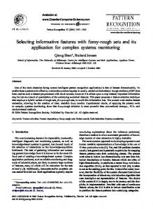
5.2.1. Efficiency Comparison. We compare the efficiencies of the backward and the sandwich algorithms. We look at only the run time of Lines 3 through 11, since these codes are the difference between two algorithms. For the course selection data set, when ms = mt = 0.06, sc = 0.18, and tc = 0.11, we obtain only 40 rules. For higher thresholds, no rule can be obtained. Therefore we use the following settings: sc = 0.18, tc = 0.11, ms = mt, and ms ∈ {0.02, 0.03, 0.04, 0.05, 0.06}. Figure 1(a) shows the actual run time in miniseconds. Figure 2(a) shows the number of basic operations, including addition and comparison of numbers. Here we observe that, for different settings, the backward algorithm is more than 2 times faster than the sandwich algorithm; it only takes less than 1/3 operations than the sandwich algorithm. For the MovieLens data set, we employ the data set with 3,800 users and 3,952 movies. We use the following settings: sc = 0.15, tc = 0.14, ms = mt, and ms ∈ {0.01, 0.02, 0.03, 0.04, 0.05}. Figure 1(b) shows the actual run time in miniseconds. Figure 2(b) shows the number of basic operations, including addition and comparison of numbers. Here we observe that, for different settings, the backward algorithm is more than 3 times faster than the sandwich algorithm; it only takes less than 1/4 operations than the sandwich algorithm. 5.2.2. Change of Number of Rules for Different Data Set Sizes. Now we study how the number of rules changes with the increase of the data set size. The experiments are undertaken only on the MovieLens data set. We use the following settings: sc = 0.15, tc = 0.14, ms ∈ {0.01, 0.02}, and |U| ∈ {500, 1, 000, 1, 500, 2, 000, 2, 500, 3, 000, 3, 500}. The number of movies is always 3,952. While selecting 𝑘 users, we always select from the first user to the 𝑘th user. First we look at the number of concepts satisfying the source confidence threshold ms. According to Figure 3(a), the number of source concepts decreases with the increase of the number of users. However, Figure 3(b) indicates that this trend may not hold. In fact, from Figure 3, the most important observation is that the number of source concepts does not vary much with the change of the number of objects. When the number of users is more than 1,500, this variation is no more than 3, which is less than 5% of the total number of concepts. Second we look at the number of granular association rules satisfying all four thresholds. Figure 4 indicates that the number of rules varies more than the number of source concepts. However, this variation is less than 20% when there are more than 1,500 users or less than 10% when there are more than 2,500 users. 5.2.3. Change of Run Time for Different Data Set Sizes. We look at the run time change with the increase of the number of users. The time complexity of the algorithm is given by (40). Since the number of movies is not changed, |SG(mt)| is fixed.

Mathematical Problems in Engineering

9

×104 4

1500

3.5

Run time (ms)

Run time (ms)

3 2.5 2 1.5

1000

500

1 0.5 0

0 0.02

0.03

0.04

0.05

0.06

0.01

0.02

0.03

0.04

0.05

0.04

0.05

ms(mt)

ms(mt)

Sandwich Backward

Sandwich Backward (a)

(b)

×109 5

×108 2

4.5

1.8

4

1.6

3.5

1.4 Basic operations

Basic operations

Figure 1: Run time information: (a) course selection, (b) MovieLens (3,800 users).

3 2.5 2

1.2 1 0.8

1.5

0.6

1

0.4

0.5

0.2

0

0 0.02

0.03

0.04 ms(mt)

0.05

0.06

0.01

0.02

0.03 ms(mt)

Sandwich Backward

Sandwich Backward (a)

(b)

Figure 2: Basic operations information: (a) course selection, (b) MovieLens (3,800 users).

Moreover, according to our earlier discussion, |SC(ms)| does not vary much for different number of users. Therefore the time complexity is nearly linear with respect to the number of users. Figure 5 validates this analysis. 5.2.4. Number of Rules for Different Thresholds. Figure 6(a) shows the number of rules decreases dramatically with the increase of 𝑚𝑠 and 𝑚𝑡. For the course selection data set, the number of rules would be 0 when ms = mt = 0.07. For the

MovieLens data set, the number of rules would be 0 when ms = mt = 0.06. 5.2.5. Performance of Cold-Start Recommendation. Now we study how the performance of cold-start recommendation varies for the training and testing sets The experiments are undertaken only on the MovieLens data set. Here we employ two data sets. One is with 1,000 users and 3,952 movies, and the other is with 3,000 users and 3,952 movies. We divide

Mathematical Problems in Engineering 136

76

134

75.5

132

75

Number of source granules

Number of source granules

10

130 128 126 124 122 500

74.5 74 73.5 73 72.5

1000

1500

2000 Users

2500

3000

72 500

3500

1000

1500

(a)

2000 Users

2500

3000

3500

2500

3000

3500

(b)

Figure 3: Number of concepts on users for MovieLens: (a) ms = 0.01, (b) ms = 0.02. 290

1250

280 270

1150

Number of rules

Number of rules

1200

1100 1050

250 240

1000 950 500

260

230

1000

1500

2000 Users

2500

3000

3500

(a)

220 500

1000

1500

2000 Users (b)

Figure 4: Number of granular association rules for MovieLens: (a) ms = 0.01, (b) ms = 0.02.

user into two parts as the training and testing set. The other settings are as follows: the training set percentage is 60%, sc = 0.15, and tc = 0.14. Each experiment is repeated 30 times with different sampling of training and testing sets, and the average accuracy is computed. Figure 7 shows that with the variation of ms and mt, the recommendation performs different. Now we observe some especially interesting phenomena from this figure as follows. (1) Figures 7(a) and 7(b) are similar in general. As the user number increases, the accuracy of recommender also increases. The reason is that we get more information from the training sets to generate much better rules for the recommendation. (2) When ms and mt are suitably set (0.03), the recommender of both data sets has the maximal accuracy. With the increase or decrease of these thresholds,

the performance of the recommendation increases or decreases rapidly. (3) The performance of the recommendation does not change much on the training and the testing sets. This phenomenon figures out that the recommender is stable. 5.3. Discussions. Now we can answer the questions proposed at the beginning of this section. (1) The backward algorithm outperforms the sandwich algorithm. The backward algorithm is more than 2 times and 3 times faster than the sandwich algorithm on the course selection and MovieLens data sets, respectively. Therefore our parametric rough sets on two universes are useful in applications.

Mathematical Problems in Engineering

11

1200

900 800 700 Run time (ms)

Run time (ms)

1000

8000

600

600 500 400 300

400

200 200 500

1000

1500

2000 Users

2500

3000

100 500

3500

1000

1500

2000

2500

3000

3500

Users

(a)

(b)

3000

1200

2500

1000

2000

800

Number of rules

Number of rules

Figure 5: Run time on MovieLens: (a) ms = 0.01, (b) ms = 0.02.

1500 1000 500

600 400 200

0 0.02

0.03

0.04 ms(mt)

0.05

0 0.01

0.06

0.02

0.03

0.04

0.05

ms(mt)

(a)

(b)

0.08

0.085

0.075

0.08

0.07

0.075

Accuracy

Accuracy

Figure 6: Number of granular association rules: (a) course selection, (b) MovieLens.

0.065 0.06 0.055 0.010

0.07 0.065

0.015

0.020

0.025 ms(mt)

Training Testing

0.030

0.035

0.040

0.06 0.010

0.015

0.020

0.025 ms(mt)

0.030

0.035

0.040

Training Testing (a)

(b)

Figure 7: Accuracy of cold-start recommendation on MovieLens: (a) 1,000 users and 3,952 movies, (b) 3,000 users and 3,952 movies.

12

Mathematical Problems in Engineering (2) The number of rules does not change much for different number of objects. Therefore it is not necessary to collect too many data to obtain meaningful granular association rules. For example, for the MovieLens data set, 3,000 users are pretty enough. (3) The run time is nearly linear with respect to the number of objects. Therefore the algorithm is scalable from the viewpoint of time complexity. However, we observe that the relation table might be rather big; therefore this would be a bottleneck of the algorithm. (4) The number of rules decreases dramatically with the increase of thresholds ms and mt. It is important to specify appropriate thresholds to obtain useful rules. (5) The performance of cold-start recommendation is stable on the training and the testing sets with the increase of thresholds ms and mt.

6. Conclusions In this paper, we have proposed a new type of parametric rough sets on two universes to deal with the granular association rule mining problem. The lower approximation operator has been defined, and its monotonicity has been analyzed. With the help of the new model, a backward algorithm for the granular association rule mining problem has been proposed. Experimental results on two real-world data sets indicate that the new algorithm is significantly faster than the existing sandwich algorithm. The performance of recommender systems is stable on the training and the testing sets. To sum up, this work applies rough set theory to recommender systems and is one step toward the application of rough set theory and granular computing. In the future, we will improve our approach and compare the performance with other recommendation approaches.

Conflict of Interests The authors declare that there is no conflict of interests regarding the publication of this paper.

Acknowledgments This work is in part supported by the National Science Foundation of China under Grant nos. 61379089, 61379049, and 61170128, the Fujian Province Foundation of Higher Education under Grant no. JK2012028, the Key Project of Education Department of Fujian Province under Grant No. JA13192, and the Postgraduate Education Innovation Base for Computer Application Technology, Signal and Information Processing of Fujian Province (no. [2008]114, High Education of Fujian).

References [1] L. Dehaspe, H. Toivonen, and R. D. King, “Finding frequent substructures in chemical compounds,” in Proceedings of the 4th International Conference on Knowledge Discovery and Data Mining, pp. 30–36, 1998.

[2] B. Goethals, W. Le Page, and M. Mampaey, “Mining interesting sets and rules in relational databases,” in Proceedings of the 25th Annual ACM Symposium on Applied Computing (SAC ’10), pp. 997–1001, March 2010. [3] S. Dˇzeroski, “Multi-relational data mining: an introduction,” in SIGKDD Explorations, vol. 5, pp. 1–16, 2003. [4] V. C. Jensen and N. Soparkar, “Frequent item set counting across multiple tables,” in Proceedings of the 4th Pacific-Asia Conference on Knowledge Discovery and Data Mining, Current Issues and New Application, vol. 1805 of Lecture Notes in Computer Science, pp. 49–61, 2000. [5] F. Min, Q. H. Hu, and W. Zhu, “Granular association rules on two universes with four measures,” 2012, http://arxiv.org/abs/ 1209.5598. [6] F. Min, Q. H. Hu, and W. Zhu, “Granular association rules with four subtypes,” in Proceedings of the IEEE International Conference on Granular Computing, pp. 432–437, 2012. [7] J. Hu and C. Guan, “An emotional agent model based on granular computing,” Mathematical Problems in Engineering, vol. 2012, Article ID 601295, 10 pages, 2012. [8] T. Y. Lin, “Granular computing on binary relations I: data mining and neighborhoodsystems,” Rough Sets in Knowledge Discovery, vol. 1, pp. 107–121, 1998. [9] J. T. Yao and Y. Y. Yao, “Information granulation for web based information retrieval support systems,” in Proceedings of SPIE, vol. 5098, pp. 138–146, April 2003. [10] Y. Y. Yao, “Granular Computing: Basic issues and possible solutions,” in Proceedings of the 5th Joint Conference on Information Sciences (JCIS ’00), vol. 1, pp. 186–189, March 2000. [11] W. Zhu and F.-Y. Wang, “Reduction and axiomization of covering generalized rough sets,” Information Sciences, vol. 152, pp. 217–230, 2003. [12] W. Zhu, “Generalized rough sets based on relations,” Information Sciences, vol. 177, no. 22, pp. 4997–5011, 2007. [13] F. Min, H. He, Y. Qian, and W. Zhu, “Test-cost-sensitive attribute reduction,” Information Sciences, vol. 181, no. 22, pp. 4928–4942, 2011. [14] F. Min, Q. Hu, and W. Zhu, “Feature selection with test cost constraint,” International Journal of Approximate Reasoning, vol. 55, no. 1, pp. 167–179, 2014. [15] A. I. Schein, A. Popescul, L. H. Ungar, and D. M. Pennock, “Methods and metrics for cold-start recommendations,” SIGIR Forum, pp. 253–260, 2002. [16] H. Guo, “Soap: live recommendations through social agents,” in Proceedings of the 5th DELOS Workshop on Filtering and Collaborative Filtering, pp. 1–17, 1997. [17] M. Balabanovi´c and Y. Shoham, “Content-based, collaborative recommendation,” Communications of the ACM, vol. 40, no. 3, pp. 66–72, 1997. [18] G. Adomavicius and A. Tuzhilin, “Toward the next generation of recommender systems: a survey of the state-of-the-art and possible extensions,” IEEE Transactions on Knowledge and Data Engineering, vol. 17, no. 6, pp. 734–749, 2005. [19] R. Burke, “Hybrid recommender systems: survey and experiments,” User Modelling and User-Adapted Interaction, vol. 12, no. 4, pp. 331–370, 2002. [20] A. H. Dong, D. Shan, Z. Ruan, L. Y. Zhou, and F. Zuo, “The design and implementationof an intelligent apparel recommend expert system,” Mathematical Problemsin Engineering, vol. 2013, Article ID 343171, 8 pages, 2013.

Mathematical Problems in Engineering [21] M. Pazzani and D. Billsus, “Content-based recommendation systems,” in The Adaptive Web, vol. 4321, pp. 325–341, Springer, 2007. [22] W. Zhu, “Relationship among basic concepts in covering-based rough sets,” Information Sciences, vol. 179, no. 14, pp. 2478–2486, 2009. [23] Y. Y. Yao and X. F. Deng, “A granular computing paradigm for concept learning,” in Emerging Paradigms in Machine Learning, vol. 13, pp. 307–326, Springer, Berlin, Germany, 2013. [24] J. Yao, “Recent developments in granular computing: a bibliometrics study,” in Proceedings of the IEEE International Conference on Granular Computing (GRC ’08), pp. 74–79, August 2008. [25] F. Aftrati, G. Das, A. Gionis, H. Mannila, T. Mielik¨ainen, and P. Tsaparas, “Mining chains of relations,” in Data Mining: Foundations and Intelligent Paradigms, vol. 24, pp. 217–246, Springer, 2012. [26] L. Dehaspe and H. Toivonen, “Discovery of frequent datalog patterns,” Expert Systems with Applications, vol. 3, no. 1, pp. 7– 36, 1999. [27] B. Goethals, W. Le Page, and H. Mannila, “Mining association rules of simple conjunctive queries,” in Proceedings of the 8th SIAM International Conference on Data Mining, pp. 96–107, April 2008. [28] W. Ziarko, “Variable precision rough set model,” Journal of Computer and System Sciences, vol. 46, no. 1, pp. 39–59, 1993. [29] T. J. Li and W. X. Zhang, “Rough fuzzy approximations on two universes of discourse,” Information Sciences, vol. 178, no. 3, pp. 892–906, 2008. [30] G. Liu, “Rough set theory based on two universal sets and its applications,” Knowledge-Based Systems, vol. 23, no. 2, pp. 110– 115, 2010. [31] S. Wong, L. Wang, and Y. Y. Yao, “Interval structure: a framework for representinguncertain information,” in Uncertainty in Artificial Intelligence, pp. 336–343, 1993. [32] Z. Pawlak, “Rough sets,” International Journal of Computer & Information Sciences, vol. 11, no. 5, pp. 341–356, 1982. [33] A. Skowron and J. Stepaniuk, “Approximation of relations,” in Proceedings of the Rough Sets, Fuzzy Sets and Knowledge Discovery, W. Ziarko, Ed., pp. 161–166, 1994. [34] Z. Pawlak, Rough Sets: Theoretical Aspects of Reasoning about Data, Kluwer Academic, Boston, Mass, USA, 1991. [35] S. K. M. Wong, L. S. Wang, and Y. Y. Yao, “On modelling uncertainty with interval structures,” Computational Intelligence, vol. 12, no. 2, pp. 406–426, 1995. [36] Y. Y. Yao and S. K. M. Wong, “A decision theoretic framework for approximating concepts,” International Journal of ManMachine Studies, vol. 37, no. 6, pp. 793–809, 1992. [37] H. X. Li, X. Z. Zhou, J. B. Zhao, and D. Liu, “Attribute reduction in decision-theoreticrough set model: a further investigation,” in Proceedings of the Rough Sets and KnowledgeTechnology, vol. 6954 of Lecture Notes in Computer Science, pp. 466–475, 2011. [38] D. Liu, T. Li, and D. Ruan, “Probabilistic model criteria with decision-theoretic rough sets,” Information Sciences, vol. 181, no. 17, pp. 3709–3722, 2011. [39] X. Y. Jia, W. H. Liao, Z. M. Tang, and L. Shang, “Minimum cost attribute reductionin decision-theoretic rough set models,” Information Sciences, vol. 219, pp. 151–167, 2013. [40] D. Liu, Y. Yao, and T. Li, “Three-way investment decisions with decision-theoretic rough sets,” International Journal of Computational Intelligence Systems, vol. 4, no. 1, pp. 66–74, 2011.

13 [41] Y. Yao and Y. Zhao, “Attribute reduction in decision-theoretic rough set models,” Information Sciences, vol. 178, no. 17, pp. 3356–3373, 2008. [42] Z. T. Gong and B. Z. Sun, “Probability rough sets model between different universes and its applications,” in Proceedings of the 7th International Conference on Machine Learning and Cybernetics (ICMLC ’08), pp. 561–565, July 2008. [43] W. Ma and B. Sun, “Probabilistic rough set over two universes and rough entropy,” International Journal of Approximate Reasoning, vol. 53, no. 4, pp. 608–619, 2012. [44] B. Sun, W. Ma, H. Zhao, and X. Wang, “Probabilistic fuzzy rough set model overtwo universes,” in Rough Sets and Current Trends in Computing, pp. 83–93, Springer, 2012. [45] Y. Y. Yao and T. Y. Lin, “Generalization of rough sets using modal logic,” Intelligent Automation and Soft Computing, vol. 2, pp. 103–120, 1996. [46] X. He, F. Min, and W. Zhu, “A comparative study of discretization approaches for granular association rule mining,” in Proceedings of the Canadian Conference on Electrical and Computer Engineering, pp. 725–729, 2013. [47] F. Min, Q. Liu, and C. Fang, “Rough sets approach to symbolic value partition,” International Journal of Approximate Reasoning, vol. 49, no. 3, pp. 689–700, 2008. [48] F. Min and W. Zhu, “Granular association rules for multi-valued data,” in Proceedings of the Canadian Conference on Electrical and Computer Engineering, pp. 799–803, 2013.

Advances in

Operations Research Hindawi Publishing Corporation http://www.hindawi.com

Volume 2014

Advances in

Decision Sciences Hindawi Publishing Corporation http://www.hindawi.com

Volume 2014

Journal of

Applied Mathematics

Algebra

Hindawi Publishing Corporation http://www.hindawi.com

Hindawi Publishing Corporation http://www.hindawi.com

Volume 2014

Journal of

Probability and Statistics Volume 2014

The Scientific World Journal Hindawi Publishing Corporation http://www.hindawi.com

Hindawi Publishing Corporation http://www.hindawi.com

Volume 2014

International Journal of

Differential Equations Hindawi Publishing Corporation http://www.hindawi.com

Volume 2014

Volume 2014

Submit your manuscripts at http://www.hindawi.com International Journal of

Advances in

Combinatorics Hindawi Publishing Corporation http://www.hindawi.com

Mathematical Physics Hindawi Publishing Corporation http://www.hindawi.com

Volume 2014

Journal of

Complex Analysis Hindawi Publishing Corporation http://www.hindawi.com

Volume 2014

International Journal of Mathematics and Mathematical Sciences

Mathematical Problems in Engineering

Journal of

Mathematics Hindawi Publishing Corporation http://www.hindawi.com

Volume 2014

Hindawi Publishing Corporation http://www.hindawi.com

Volume 2014

Volume 2014

Hindawi Publishing Corporation http://www.hindawi.com

Volume 2014

Discrete Mathematics

Journal of

Volume 2014

Hindawi Publishing Corporation http://www.hindawi.com

Discrete Dynamics in Nature and Society

Journal of

Function Spaces Hindawi Publishing Corporation http://www.hindawi.com

Abstract and Applied Analysis

Volume 2014

Hindawi Publishing Corporation http://www.hindawi.com

Volume 2014

Hindawi Publishing Corporation http://www.hindawi.com

Volume 2014

International Journal of

Journal of

Stochastic Analysis

Optimization

Hindawi Publishing Corporation http://www.hindawi.com

Hindawi Publishing Corporation http://www.hindawi.com

Volume 2014

Volume 2014