Research Article Parareal Algorithms Implemented ...

Hindawi Publishing Corporation Mathematical Problems in Engineering Volume 2015, Article ID 395340, 12 pages http://dx.doi.org/10.1155/2015/395340

Research Article Parareal Algorithms Implemented with IMEX Runge-Kutta Methods Zhiyong Wang1 and Shulin Wu2 1

School of Mathematical Sciences, University of Electronic Science and Technology of China, Chengdu, Sichuan 610731, China School of Science, Sichuan University of Science and Engineering, Zigong, Sichuan 643000, China

2

Correspondence should be addressed to Zhiyong Wang; [email protected] Received 17 June 2014; Revised 31 August 2014; Accepted 1 September 2014 Academic Editor: Zhike Peng Copyright © 2015 Z. Wang and S. Wu. This is an open access article distributed under the Creative Commons Attribution License, which permits unrestricted use, distribution, and reproduction in any medium, provided the original work is properly cited. Parareal algorithm is a very powerful parallel computation method and has received much interest from many researchers over the past few years. The aim of this paper is to investigate the performance of parareal algorithm implemented with IMEX Runge-Kutta (RK) methods. A stability criterion of the parareal algorithm coupled with IMEX RK methods is established and the advantage (in the sense of stability) of implementing with this kind of RK methods is numerically investigated. Finally, numerical examples are given to illustrate the efficiency and performance of different parareal methods.

1. Introduction The parareal algorithm was presented by Lions et al. in [1] as a numerical method to solve time dependent problems in parallel. The peculiarity of this algorithm is that it approximates successfully the solution later in time before having fully accurate approximations from earlier time points. This algorithm is becoming more and more popular in scientific and engineering computation and many excellent results have been obtained. As mentioned above, the parareal algorithm was first introduced in [1] and an improved version which aims to solve nondifferentiable PDEs was discussed by Bal and Maday in [2]. Some further modifications and improvements can be found in [3], in which the authors use the “filtering” technique to overcome the so-called resonance or beating phenomenon (see also [4, 5]) that triggers numerical instability when the algorithm is applied to linear structure dynamics. The stability and convergence are the main subjects of theoretical analysis of the algorithm which have been investigated widely by many researchers; see, for example, [6–8]. Nowadays, this algorithm, as well as its variants [3, 9–12], has been used in many fields by many researchers, such as morphological transformation simulations [13], structural (fluid) dynamics

simulations [4, 5, 14], optimal control [15, 16], Hamiltonian simulations [17, 18], turbulent plasma simulations [19, 20], and solution of Volterra integral equations [21]. (There is an increasing interest in parareal, and it is very possible that some important references are not mentioned here.) For ODEs, 𝑦󸀠 (𝑡) = 𝑓 (𝑡, 𝑦 (𝑡)) , 𝑦 (0) = 𝑦0 ,

𝑡 ∈ [0, 𝑇] ,

(1)

to formulate the parareal algorithm, the time domain [0, 𝑇] of interest is first partitioned into several time-slices whose boundary points are treated as coarse time-grids. And then, the algorithm consists of three basic steps. First, using some numerical propagator, say GΔ𝑇, the solution is approximated on each coarse time-grid to provide a seed—that is, an initial condition—to the time-slice. Second, another propagator, denoted by FΔ𝑡 , is applied independently and therefore concurrently in each time-slice to advance the solution from the starting point of this time-slice to its end point. Finally, an iterative process is invoked to improve the accuracy of the seeds and eliminate the jumps of the solution on the coarse time-grids. In most cases, the numerical propagators GΔ𝑇 and FΔ𝑡 are defined by traditional RK method with

2

Mathematical Problems in Engineering

equal length of the time-slices, such as Radau methods, Lobatto methods, and Gauss methods, and there are lots of investigations about theoretical properties and performance of practical application of the algorithm in such case. See, for example, [4, 5, 7, 9, 14] and references therein. There is also some research about special choice of the underlying numerical methods that are used to define GΔ𝑇 and FΔ𝑡 . For example, Guibert and Tromeur-Dervout [22] considered the adaptive time-slices (i.e., the length of timeslices is not equal) to define GΔ𝑇 and FΔ𝑡 and the derived parareal algorithm can be applied to strong stiff ODEs and differential algebraic equations (DAEs). Another example is the one investigated by Minion [11], where the authors defined the numerical propagators GΔ𝑇 and FΔ𝑡 by spectral deferred correction based on the Gaussian quadrature spectral integration. It was shown that the iterative process based on spectral deferred correction rather than traditional methods within a parareal framework results in a significant decrease in the overall computational cost of the algorithm. Wu et al. [9] suggested that the propagator FΔ𝑡 was defined by local Richardson extrapolation, and it turns out that the Parareal-Richardson method has advantages of higher accuracy and better stability. In some cases, the function 𝑓 in (1) can be written into two parts

different IMEX RK methods and the corresponding advantages/disadvantages are numerically shown. Finally, in Section 4, we test the Gray-Scott model arising in chemical reaction to illustrate our results.

2. The Parareal Algorithm and the IMEX RK Methods In this section, we revisit the parareal algorithm and the IMEX RK methods. 2.1. The Parareal Algorithm. To introduce the parareal algorithm, let us first partition time interval [0, 𝑇] into 𝑁 subintervals 𝑆𝑛 = [𝑇𝑛 , 𝑇𝑛+1 ], 𝑛 = 0, 1, . . . , 𝑁 − 1, with equal length Δ𝑇 and 𝑇𝑛 = 𝑛Δ𝑇. We call 𝑇𝑛 ’s the coarse time-grids. We then use some finer step size Δ𝑡 = Δ𝑇/𝑀 (𝑀 > 1 is an integer) to partition each relative large interval 𝑆𝑛 into 𝑀 finer intervals 𝑠𝑛,𝑚 = [𝑇𝑛+𝑚/𝑀, 𝑇𝑛+(𝑚+1)/𝑀] with 𝑇𝑛+𝑚/𝑀 = 𝑇𝑛 +𝑚Δ𝑡 and 𝑚 = 0, 1, . . . , 𝑀 − 1. Now, the parareal algorithm can be described as follows. We designate by symbol ⊖ the timesequential steps performed on the coarse time-grids and by symbol ⊕ the parallel steps performed on the decomposed finer time-grids. The Parareal Algorithm. Consider the following.

𝑓 = 𝑓𝑠 + 𝑓𝑛𝑠 ,

(2)

where 𝑓𝑛𝑠 is the nonstiff or mildly stiff part of 𝑓 and 𝑓𝑠 is the stiff part. A common example for such case arises from semidiscretization of reaction diffusion equations 𝑢𝑡 = 𝑑𝑢𝑥𝑥 + 𝑟(𝑡, 𝑥, 𝑢). In this case the function 𝑓 in (1) can be written as 𝑓(𝑡, 𝑦(𝑡)) = 𝐴𝑦(𝑡) + 𝑓𝑛𝑠 (𝑡, 𝑦(𝑡)) with 𝐴 being a tridiagonal matrix and stiff. In the case that 𝑓 can be partitioned into stiff and nonstiff parts, it is more advisable to use the implicitexplicit (IMEX) RK methods (or additive RK methods called sometimes) to solve ODEs (1). For this type of RK methods, the stiff part is assigned with the implicit component of the IMEX RK method to satisfy stability requirement and the nonstiff or mildly stiff part is assigned with the explicit component to reduce computational cost. For more details about the RK methods and the IMEX RK methods, the interested reader may refer to [23–33] and references therein. Therefore, under condition (2), we think that it is valuable to adopt the IMEX RK methods instead of the traditional RK methods to define GΔ𝑇 and/or FΔ𝑡 used in parareal framework. This is the main motivation of our work. In certain aspects, this paper should be viewed as an experimental one. While the stability of the derived algorithm we present is easily proven by the results given by Gander and Vandewalle [7], stability region of the parareal algorithm defined by the IMEX RK methods is numerically shown. The structure of this paper is as follows. In Section 2, the parareal algorithm and the IMEX RK methods are revisited. Section 3 is concerned with the stability of the derived parareal algorithm. Several combinations of

⊖ Step 0 (initialization). Perform sequential computation 0 = GΔ𝑇 (𝑇𝑛 , 𝑌𝑛0 , Δ𝑇) with 𝑌00 = 𝑦0 , 𝑛 = 0, 1, . . . , 𝑁 − 1, 𝑌𝑛+1 for 𝑘 = 0, 1, . . .. ⊕ Step 1. Perform in subinterval 𝑆𝑛 = [𝑇𝑛 , 𝑇𝑛+1 ] the computâ𝑛+(𝑚+1)/𝑀 = FΔ𝑡 (𝑇𝑛+𝑚/𝑀, 𝑌 ̂𝑛+𝑚/𝑀, Δ𝑡) with initial value tion 𝑌 𝑘 𝑌𝑛 , 𝑚 = 0, 1, . . . , 𝑀 − 1. 𝑘+1 ⊖ Step 2. Perform sequential corrections 𝑌𝑛+1 = GΔ𝑇 (𝑇𝑛 , ̂𝑛+1 − GΔ𝑇(𝑇𝑛 , 𝑌𝑘 , Δ𝑇) with 𝑌𝑘+1 = 𝑦0 , 𝑛 = 0, 𝑌𝑛𝑘+1 , Δ𝑇) + 𝑌 𝑛 0 1, . . . , 𝑁 − 1.

⊖ Step 3. If for 𝑛 = 0, 1, . . . , 𝑁 − 1, 𝑌𝑛𝑘+1 satisfy some termination criteria, stop the iteration; else go to Step 1. Here, the finer propagation operator FΔ𝑡 and the coarse propagation operator GΔ𝑇 relay on one-step numerical methods and if the underlying methods are implicit, in most cases (linear ODEs is an exception), nonlinear algebraic equations need to be solved. The above algorithm can be written compactly as 𝑘+1 = GΔ𝑇 (𝑇𝑛 , 𝑌𝑛𝑘+1 , Δ𝑇) + FΔ𝑡 (𝑇𝑛 , 𝑌𝑛𝑘 , Δ𝑡) 𝑌𝑛+1

− GΔ𝑇 (𝑇𝑛 , 𝑌𝑛𝑘 , Δ𝑇) ,

(3)

where 𝑘 is the iteration index. Note that for 𝑘 → +∞ method (3) will generate a series of values 𝑌𝑛 which satisfy 𝑌𝑛+1 = FΔ𝑡 (𝑇𝑛 , 𝑌𝑛 , Δ𝑡). This implies that the converged solution 𝑌𝑛 will achieve the accuracy of the propagator FΔ𝑡 .

Mathematical Problems in Engineering

3 𝑠

2.2. The IMEX RK Methods. Let us consider a pair of two Runge-Kutta methods defined by the arrays 0 0 0 𝑐2 𝑎21 𝑎22

0 0

⋅⋅⋅ ⋅⋅⋅

𝑐3 𝑎̂31 .. .. . . 𝑐𝑠 𝑎̂𝑠1 ̂𝑏 1

0 0

0 0

⋅⋅⋅ ⋅⋅⋅

0 𝑎̂32 0 .. .. . . d 𝑎̂𝑠2 ⋅ ⋅ ⋅ 𝑎̂𝑠,𝑠−1 ̂𝑏 ⋅ ⋅ ⋅ ̂𝑏 2 𝑠−1

+ ℎ∑̂𝑏𝑗 𝑓𝑛𝑠 (𝑡𝑛 + 𝑐𝑗 ℎ, 𝐾𝑗 ) ,

0 0 .. .

𝑗=1

(7)

(4)

0 0 .. . 0 0 ̂𝑏

𝑠

𝑖

𝑖−1

𝑗=1

𝑖 = 2, . . . , 𝑠.

0 0 0 0 0 0 1 0 1 1 1 0 0 1 1 0 ⏟⏟⏟⏟⏟⏟⏟⏟⏟⏟⏟⏟⏟⏟⏟⏟⏟⏟⏟⏟⏟⏟⏟⏟⏟⏟⏟⏟⏟⏟⏟⏟⏟

(5)

𝑗=1

The top formula of (4) determines a diagonally implicit (semi-implicit) RK method and the bottom formula is an explicit RK method. In addition, let ℎ > 0 be a step size and define the step point 𝑡𝑛 = 𝑛ℎ for integer 𝑛. Consider the following stiff/nonstiff partitioned ODEs: 󸀠

𝑦 (𝑡) = 𝑓𝑠 (𝑡, 𝑦 (𝑡)) + 𝑓𝑛𝑠 (𝑡, 𝑦 (𝑡)) ,

𝑡 ∈ [0, 𝑇] ,

𝑦 (0) = 𝑦0 ,

𝑖

𝐾𝑖 = 𝑦𝑛 + ℎ∑ 𝑎𝑖𝑗 𝑓𝑠 (𝑡𝑛 + 𝑐𝑗 ℎ, 𝐾𝑗 ) 𝑗=1

+ ℎ∑ 𝑎̂𝑖𝑗 𝑓𝑛𝑠 (𝑡𝑛 + 𝑐𝑗 ℎ, 𝐾𝑗 ) ,

(8)

IMEX Euler

Second Order IMEX RK Methods. The second order IMEX RK methods considered here are the IMEX trapezoidal scheme [34]: 0 0 0 0 0 0 1 1 1 1 1 0 2 2 1 1 1 1 2 2 ⏟⏟⏟⏟⏟⏟⏟⏟⏟⏟⏟⏟⏟⏟⏟⏟⏟⏟⏟⏟⏟⏟⏟⏟⏟⏟⏟⏟⏟⏟⏟⏟⏟⏟⏟⏟⏟⏟⏟ 2 2

(6)

and by applying the top part of (4) to stiff component 𝑓𝑠 and the bottom part to the nonstiff component, we obtain the following scheme:

𝑖−1

where ∑𝑖𝑗=1 (⋅) = 0 with 𝑖 < 𝑗. The order conditions for IMEX RK methods are very complicated and beyond the topic of this paper. For this aspect, we refer the interested reader to, for example, [26, 30]. At the moment, we introduce some frequently used IMEX methods with order 𝑝 = 1, 2, 3. We will use the triplet IMEX(𝑠im , 𝑠ex , 𝑝) to identify scheme (4), where 𝑠im is the number of stages of the implicit part, 𝑠ex is the number of stages of the explicit part, and 𝑝 is the order of the IMEX scheme. First Order IMEX RK Methods. The most popular first order IMEX RK method is the IMEX Euler method:

with the same abscissae 𝑐𝑖 = ∑𝑎𝑖𝑗 = ∑𝑎̂𝑖𝑗 ,

𝑗=1

𝑠

𝑐3 𝑎31 𝑎32 𝑎33 0 .. .. .. .. . . . . d 0 𝑐𝑠 𝑎𝑠1 𝑎𝑠2 ⋅ ⋅ ⋅ 𝑎𝑠,𝑠−1 𝑎𝑠𝑠 𝑏1 𝑏2 ⋅ ⋅ ⋅ 𝑏𝑠−1 𝑏𝑠 0 0 𝑐2 𝑎̂21

𝑦𝑛+1 = 𝑦𝑛 + ℎ∑ 𝑏𝑗 𝑓𝑠 (𝑡𝑛 + 𝑐𝑗 ℎ, 𝐾𝑗 )

(9)

IMEX trapezoidal

The IMEX trapezoidal scheme is a combination of the trapezoidal rule and Heun’s second order method (the explicit trapezoidal rule). Third Order IMEX RK Methods. For third order IMEX RK method, we consider the one constructed by Ascher et al. [23] (this scheme is denoted by IMEX(4, 4, 3)):

𝑖 = 1, 2, . . . , 𝑠,

𝑗=1

0 0 0 0 0 0 0 0 0 0 𝑎 0 0 𝑎 0 0 0 𝑎 𝑎 0 0.3212788860 0.3966543747 0 0 0.7179332607 0 0.2820667392 0 1.2084966490 −0.644363171 𝑎 −0.1058858296 𝑏 𝑏 0 1 0 1.2084966490 −0.644363171 𝑎 ⏟⏟⏟⏟⏟⏟⏟⏟⏟⏟⏟⏟⏟⏟⏟⏟⏟⏟⏟⏟⏟⏟⏟⏟⏟⏟⏟⏟⏟⏟⏟⏟⏟⏟⏟⏟⏟⏟⏟⏟⏟⏟⏟⏟⏟⏟⏟⏟⏟⏟⏟⏟⏟⏟⏟⏟⏟⏟⏟⏟⏟⏟⏟⏟⏟⏟⏟⏟⏟⏟⏟⏟⏟⏟⏟⏟⏟⏟⏟⏟⏟⏟⏟⏟⏟⏟⏟⏟⏟⏟⏟⏟⏟⏟⏟⏟⏟⏟⏟⏟⏟⏟⏟ 0 1.2084966490 −0.644363171 𝑎⏟⏟ ⏟⏟⏟⏟⏟⏟⏟⏟⏟⏟⏟⏟⏟⏟⏟⏟⏟⏟⏟⏟⏟⏟⏟⏟⏟⏟⏟⏟⏟⏟⏟⏟⏟⏟⏟⏟⏟⏟⏟⏟⏟⏟⏟⏟⏟⏟⏟⏟⏟⏟⏟⏟⏟⏟⏟⏟⏟⏟⏟⏟⏟⏟⏟⏟⏟⏟⏟⏟⏟⏟⏟⏟⏟⏟⏟⏟⏟⏟⏟⏟⏟⏟⏟⏟⏟⏟⏟⏟⏟⏟⏟⏟⏟⏟⏟⏟⏟⏟⏟⏟⏟⏟

(10)

IMEX(4,4,3)

where 𝑎 = 0.4358665215 and 𝑏 = 0.552929147. Both the implicit and explicit schemes of IMEX(4, 4, 3) are third order RK methods, and the implicit scheme is 𝐿-stable.

To finish this section, we introduce the concept of stability of the IMEX RK methods which will be used in the stability analysis of the parareal algorithm.

4

Mathematical Problems in Engineering

The asymptotic behavior of the IMEX RK methods applied to (6) is analyzed on the basis of the scalar model equation: 𝑦󸀠 (𝑡) = 𝜆𝑦 + 𝜇𝑦,

𝜆, 𝜇 ∈ C,

(11)

and FΔ𝑡 are 𝑅F (𝛼, 𝛽) and 𝑅G (𝛼, 𝛽), respectively. Then it follows by applying the parareal algorithm to the model equation (11) that GΔ𝑇 (𝑇𝑛 , 𝑌𝑛𝑘 , Δ𝑇) = 𝑅G (𝛼, 𝛽) 𝑌𝑛𝑘 ,

which was proposed by Frank et al. [35] and Verwer and Sommeijer [36] and adopted by Koto [28, 37]. For model equation (11), from (7) we arrive at

𝑀 FΔ𝑡 (𝑇𝑛 , 𝑌𝑛𝑘 , Δ𝑇) = 𝑅F (

̂ 𝐾 = E𝑦𝑛 + ℎ𝜆𝐴𝐾 + ℎ𝜇𝐴𝐾,

where we recall 𝑀 = Δ𝑇/Δ𝑡.

(12)

̂ 𝑦𝑛+1 = 𝑦𝑛 + ℎ𝜆b𝐾 + ℎ𝜇b𝐾,

where we have used vector and matrix notations to denote the ̂= values shown in the Butcher tableau (4); that is, 𝐴 = (𝑎𝑖𝑗 ), 𝐴 ̂ = (̂𝑏 , ̂𝑏 , . . . , ̂𝑏 ). Moreover, ̂𝑖𝑗 ), b = (𝑏1 , 𝑏2 , . . . , 𝑏𝑠 ), and b (𝐴 1 2 𝑠 𝑇 E = (1, 1, . . . , 1) . Let 𝛼 = ℎ𝜆, 𝛽 = ℎ𝜇. We then have 𝑦𝑛+1 = 𝑅 (𝛼, 𝛽) 𝑦𝑛 ,

(13)

where 𝑅(𝛼, 𝛽) is called stability function of the IMEX RK method which is defined by −1

̂ (𝐼 − 𝛼𝐴 − 𝛽𝐴) ̂ E, 𝑅 (𝛼, 𝛽) = 1 + (𝛼b + 𝛽b)

3. Stability of the Parareal Algorithm In our analysis of the stability of the parareal algorithm implemented with IMEX RK methods, an important role is a strictly lower triangular Toeplitz matrix M := M(𝜎) of size 𝑁. Its elements are defined by if 𝑖 ≤ 𝑗, if 𝑖 > 𝑗.

(15)

The next necessity for our analysis is the estimation of ‖M𝑘 ‖∞ , which is proved by Gander and Vandewalle [7]. Lemma 1 (see [7]). Let 𝑘 > 0 be an integer. Then the infinite norm of M𝑘 can be estimated by 󵄩󵄩 𝑘 󵄩󵄩 󵄩󵄩M (𝜎)󵄩󵄩 󵄩 󵄩∞ 𝑁−1

𝑘

𝑁−1 1 − |𝜎| { { )} , 𝑖𝑓 |𝜎| < 1, ) ,( min {( { { 𝑘 1 − |𝜎| { ≤{ { { { {|𝜎|𝑁−𝑘−1 (𝑁 − 1) , 𝑖𝑓 |𝜎| ≥ 1. 𝑘 { (16) Assume that the stability functions of the underlying numerical methods used to define the two propagators GΔ𝑇

𝑘 = 1, 2, . . . ,

(17)

Theorem 2. Let Δ𝑇 be given and 𝑇𝑛 = 𝑛Δ𝑇 for 𝑛 = 0, 1, . . .. Let the underlying numerical method used to define the propagator GΔ𝑇 running on the coarse time-grids be in its region of absolute stability; that is, |𝑅G | < 1. Then one has the following estimates: 󵄨 󵄨 sup 󵄨󵄨󵄨󵄨𝑦 (𝑡𝑛 ) − 𝑌𝑛𝑘 󵄨󵄨󵄨󵄨 𝑛>0

󵄨󵄨 𝑀 󵄨 𝑘 󵄨󵄨𝑅F (𝛼/𝑀, 𝛽/𝑀) − 𝑅G (𝛼, 𝛽)󵄨󵄨󵄨 󵄨 󵄨 ) sup 󵄨󵄨󵄨𝑦 (𝑡 ) − 𝑌0 󵄨󵄨󵄨 , ≤( 󵄨󵄨 𝑛 󵄨 󵄨 𝑛 󵄨󵄨 1 − 󵄨󵄨󵄨𝑅G (𝛼, 𝛽)󵄨󵄨󵄨 𝑛>0 𝑘 ≥ 1. (18)

(14)

where 𝐼 is an identity matrix of size 𝑠.

0, M𝑖𝑗 = { 𝑖−𝑗−1 𝜎 ,

𝛼 𝛽 , ) 𝑌𝑘 , 𝑀 𝑀 𝑛

Proof. We denote by 𝑒𝑛𝑘 the error at iteration 𝑘 of the parareal algorithm at coarse time point 𝑇𝑛 ; that is, 𝑒𝑛𝑘 = 𝑦(𝑡𝑛 ) − 𝑌𝑛𝑘 . Then with an induction argument on 𝑛, it follows by applying the iterative process (3) to the model equation (11) that this error satisfies 𝑘+1 = 𝑅G (𝛼, 𝛽) 𝑒𝑛𝑘+1 + [𝑅F ( 𝑒𝑛+1

𝛼 𝛽 , ) − 𝑅G (𝛼, 𝛽)] 𝑒𝑛𝑘 𝑀 𝑀

𝑛 𝛼 𝛽 𝑛−𝑗 = [𝑅F ( , ) − 𝑅G (𝛼, 𝛽)] ∑𝑅G (𝛼, 𝛽) 𝑒𝑗𝑘 , 𝑀 𝑀 𝑗=1

(19)

where we have used the fact that 𝑒0𝑘 = 0 for any 𝑘 ≥ 0. Set 𝑘 𝑇 ) . Then relation (19) can be written in 𝐸𝑘 = (𝑒1𝑘 , 𝑒2𝑘 , . . . , 𝑒𝑁 matrix form as 𝐸𝑘+1 = [𝑅F (

𝛼 𝛽 , ) − 𝑅G (𝛼, 𝛽)] M (𝑅G (𝛼, 𝛽)) 𝐸𝑘 , 𝑀 𝑀 (20)

where the matrix M is defined by (15) with 𝜎 = 𝑅G (𝛼, 𝛽). This implies

𝐸𝑘 = [𝑅F (

𝑘 𝛼 𝛽 , ) − 𝑅G (𝛼, 𝛽)] M𝑘 (𝑅G (𝛼, 𝛽)) 𝐸0 . (21) 𝑀 𝑀

Mathematical Problems in Engineering

5

Therefore, from Lemma 1 and the assumption |𝑅G | < 1, we have 󵄨󵄨 󵄨󵄨𝑘 𝛼 𝛽 󵄩󵄩 𝑘 󵄩󵄩 󵄩󵄩𝐸 󵄩󵄩 ≤ 󵄨󵄨󵄨󵄨𝑅F ( , ) − 𝑅G (𝛼, 𝛽)󵄨󵄨󵄨󵄨 󵄩 󵄩∞ 󵄨󵄨 󵄨󵄨 𝑀 𝑀 󵄩 󵄩󵄩 󵄩 × 󵄩󵄩󵄩󵄩M𝑘 (𝑅G (𝛼, 𝛽))󵄩󵄩󵄩󵄩 󵄩󵄩󵄩󵄩𝐸0 󵄩󵄩󵄩󵄩∞ 󵄨󵄨 󵄨󵄨𝑘 𝛼 𝛽 󵄨 󵄨 ≤ 󵄨󵄨󵄨𝑅F ( , ) − 𝑅G (𝛼, 𝛽)󵄨󵄨󵄨 󵄨󵄨 󵄨󵄨 𝑀 𝑀 ×(

PIM-EX : GΔ𝑇 is defined by the implicit part of IMEXG and FΔ𝑡 is defined by the explicit part IMEXF ; (22)

󵄨𝑁−1 𝑘 󵄨 1 − 󵄨󵄨󵄨𝑅G (𝛼, 𝛽)󵄨󵄨󵄨 󵄩󵄩 0 󵄩󵄩 󵄨 󵄨 ) 󵄩󵄩󵄩𝐸 󵄩󵄩󵄩∞ . 1 − 󵄨󵄨󵄨𝑅G (𝛼, 𝛽)󵄨󵄨󵄨

PIM-IMEX : GΔ𝑇 is defined by the implicit component of IMEXG and FΔ𝑡 is defined by IMEXF ; PIMEX-EX : GΔ𝑇 is defined by IMEXG and FΔ𝑡 is defined by the explicit component of IMEXF ;

Hence, the proof of this theorem is completed by letting 𝑁 → +∞ in the second inequality of (22). 𝑀 The factor 𝜌(𝛼, 𝛽) := |𝑅F (𝛼/𝑀, 𝛽/𝑀) − 𝑅G (𝛼, 𝛽)|/(1 − |𝑅G (𝛼, 𝛽)|) is called by Gander and Vandewalle [7] the linear convergence factor of the parareal algorithm performed on unbounded time intervals. According to the concepts introduced by Bal [6] and Staff and Rønquist [8], it is also called the stability function of the parareal algorithm. In this paper, we use the latter name. Define

D = {(𝛼, 𝛽) | 𝜌 (𝛼, 𝛽) < 1, 𝛼, 𝛽 ∈ C} .

To see whether our desirability can be carried through, for two IMEX RK methods, IMEXG and IMEXF , we consider here 𝑀 = 50 and the following four special combinations which leads to four parareal algorithms:

(23)

Then if (𝛼, 𝛽) ∈ D, the parareal algorithm is convergent on unbounded time intervals. In what follows of this paper, the set D is called stability region of the parareal algorithm. ̂ and 𝐴 = 𝐴 ̂ (i.e., the IMEX RK methods Remark 3. If b = b reduce to the traditional RK methods), it follows from (14) that 𝑅(𝛼, 𝛽) = R(𝑧) = 1 + 𝑧b(𝐼 − 𝑧𝐴)−1 E with 𝑧 = 𝛼 + 𝛽. Therefore, if both the propagators GΔ𝑇 and FΔ𝑡 are defined by the traditional RK methods, the stability function 𝜌(𝛼, 𝛽) ̃ = |R𝑀 can be rewritten as 𝜌(𝑧) F (𝑧/𝑀)−RG (𝑧)|/(1−|RG (𝑧)|), which is the one obtained by Gander and Vandewalle in [7]. From Remark 3, we see that the underlying numerical method used to define propagator GΔ𝑇 that is in its absolute stability region is necessary for the stability of the parareal algorithm. In fact, in the previous analysis and application of the parareal algorithm (i.e., both the propagators GΔ𝑇 and FΔ𝑡 are defined by the traditional RK methods), it has been proposed by Farhat et al. [4, 5, 14] that the underlying RK method for GΔ𝑇 should be implicit and the one for the propagator FΔ𝑡 should be explicit. The reason is obvious— the implicit RK method is used to guarantee stability and the explicit RK method is used to reduce computation cost as much as possible. The greatest advantage of using an IMEX RK method is that the stability of the combined scheme approaches to that of its implicit part while the computational cost can bear comparison with simply using the explicit part. Hence, in the parareal framework, it is naturally desired that the adoption of the IMEX RK methods will provide a far more stable parareal algorithm with computational cost sharply reduced.

PIMEX-IMEX : GΔ𝑇 is defined by IMEXG and FΔ𝑡 is defined by IMEXF . For the convenience of plotting the stability region of the parareal algorithm, we consider the case (𝛼, 𝛽) = (𝑥, 𝑖𝑦), 𝑥, 𝑦 ∈ R. The stability functions of the above four parareal algorithms are denoted by RIM-EX (𝑥, 𝑦), RIM-IMEX (𝑥, 𝑦), RIMEX-EX (𝑥, 𝑦), and RIMEX-IMEX (𝑥, 𝑦), respectively. The stability regions are denoted by DIM-EX , DIM-IMEX , DIMEX-EX , and DIMEX-IMEX , respectively. We remark that the PIM-EX algorithm is a conventional parareal algorithm and we will compare its stability region with the ones of the other three algorithms. We first illustrate the stability regions of the parareal algorithms when IMEXG is chosen as the IMEX Euler method (see (8)). For IMEXF = IMEX Euler and IMEXF = IMEX Trapezoidal and IMEXF = IMEX(4, 4, 3), the stability region of the algorithms PIM-EX , PIM-IMEX , PIMEX-EX , and PIMEX-IMEX is plotted in Figures 1(a), 1(b), and 1(c), respectively. For IMEXG = IMEX Euler, the stability functions of the parareal algorithms shown in Figures 1(a) and 1(b) are Figure 1(a): RIM-EX (𝑥, 𝑦) 󵄨󵄨 󵄨 󵄨󵄨1/ (𝑥 + 𝑖𝑦 − 1) − (1 + (𝑥 + 𝑖𝑦)/𝑀)𝑀󵄨󵄨󵄨 󵄨, =󵄨 󵄨 󵄨 1 − 󵄨󵄨󵄨1/ (𝑥 + 𝑖𝑦 − 1)󵄨󵄨󵄨 RIM-IMEX (𝑥, 𝑦) 󵄨󵄨 󵄨 󵄨󵄨1/ (𝑥 + 𝑖𝑦 − 1) − ((𝑀 + 𝑖𝑦)/ (𝑀 − 𝑥))𝑀󵄨󵄨󵄨 󵄨 󵄨, = 󵄨 󵄨 1 − 󵄨󵄨󵄨1/ (𝑥 + 𝑖𝑦 − 1)󵄨󵄨󵄨 RIMEX-EX (𝑥, 𝑦) 󵄨󵄨 󵄨 󵄨󵄨(1 + 𝑖𝑦) / (1 − 𝑥) − (1 + (𝑥 + 𝑖𝑦)/𝑀)𝑀󵄨󵄨󵄨 󵄨, =󵄨 󵄨 󵄨 1 − 󵄨󵄨󵄨(1 + 𝑖𝑦) / (1 − 𝑥)󵄨󵄨󵄨 RIMEX-IMEX (𝑥, 𝑦) 󵄨󵄨 󵄨 󵄨󵄨(1 + 𝑖𝑦) / (1 − 𝑥) − ((𝑀 + 𝑖𝑦)/ (𝑀 − 𝑥))𝑀󵄨󵄨󵄨 󵄨 󵄨, = 󵄨 󵄨 1 − 󵄨󵄨󵄨(1 + 𝑖𝑦) / (1 − 𝑥)󵄨󵄨󵄨

Mathematical Problems in Engineering

100

𝒟IM-IMEX

40

60

60

30

40

40

20

100

20

20

10

20

0

0

0

0

0

0

−10

−100

−20

−20

−10

−20

−40

−40

−20

−60

−60

−30

100

10

0

−100

−40

−400

−100

−100

−50

(a)

0

−400

−500

−40

−1000

−80 0

−80 −50

−300

−100

−30

0

−300

−500

−200

−1000

−20

0

−200

60 40

−40 −60 −80 −1000

200

0

20

−50

200

(b)

600

60

400

50

200

20

200

0

0

0

0

−50

−200

−20

−200

−100

−400

−40

−400

−150

−600

0

−100

−200

0

−2000

−60 −4000

0

40

−100

400

−600

𝒟IMEX-IMEX

0

𝒟IMEX-EX

𝒟IM-IMEX

−2000

600

−4000

𝒟IM-EX

100

−200

𝒟IMEX-IMEX 80

80

300

150

𝒟IMEX-EX

50

0

𝒟IM-EX

100 80

30

−50

0

−50

−60

−100

−40

𝒟IMEX-IMEX 400

300

0

−20

𝒟IMEX-EX

−100

20

40

0

40

𝒟IM-IMEX

−100

400

−500

𝒟IM-EX

−1000

60

−500

6

(c)

Figure 1: (a) (IMEXG , IMEXF ) = (IMEX Euler, IMEX Euler). (b) (IMEXG , IMEXF ) = (IMEX Euler, IMEX Trapezoidal). (c) (IMEXG , IMEXF ) = (IMEX Euler, IMEX(4, 4, 3)).

Figure 1(b): RIM-EX (𝑥, 𝑦) 󵄨󵄨 𝑀 󵄨󵄨 󵄨󵄨 󵄨󵄨 𝑥 + 𝑖𝑦 (𝑥 + 𝑖𝑦)2 1 󵄨󵄨 ) = 󵄨󵄨󵄨󵄨 − (1 + + 󵄨󵄨 2 𝑀 2𝑀 󵄨󵄨 󵄨󵄨 𝑥 + 𝑖𝑦 − 1 󵄨 󵄨 −1 󵄨󵄨 󵄨 󵄨󵄨 1 󵄨 󵄨󵄨) , × (1 − 󵄨󵄨󵄨 󵄨󵄨 𝑥 + 𝑖𝑦 − 1 󵄨󵄨󵄨 RIM-IMEX (𝑥, 𝑦) 󵄨󵄨 𝑀 󵄨󵄨 󵄨󵄨 󵄨󵄨 (2 + 𝑖 (𝑦/𝑀)) (𝑥 + 𝑖𝑦) 1 = 󵄨󵄨󵄨 − (1 + ) 󵄨󵄨󵄨 󵄨󵄨 𝑥 + 𝑖𝑦 − 1 󵄨󵄨 2𝑀 − 𝑥 󵄨 󵄨 󵄨󵄨 󵄨󵄨 −1 1 󵄨 󵄨󵄨 × (1 − 󵄨󵄨󵄨 󵄨) , 󵄨󵄨 𝑥 + 𝑖𝑦 − 1 󵄨󵄨󵄨

RIMEX-EX (𝑥, 𝑦) 󵄨󵄨 2 𝑀 󵄨󵄨󵄨 󵄨󵄨 1 + 𝑖𝑦 󵄨󵄨 𝑥 + 𝑖𝑦 (𝑥 + 𝑖𝑦) 󵄨󵄨 = 󵄨󵄨 ) 󵄨󵄨󵄨 − (1 + + 2 󵄨󵄨 󵄨󵄨 1 − 𝑥 𝑀 2𝑀 󵄨󵄨 󵄨󵄨 󵄨󵄨 1 + 𝑖𝑦 󵄨󵄨 −1 󵄨 󵄨󵄨 × (1 − 󵄨󵄨󵄨 󵄨) , 󵄨󵄨 1 − 𝑥 󵄨󵄨󵄨 RIMEX-IMEX (𝑥, 𝑦) 󵄨󵄨 𝑀 󵄨󵄨 󵄨󵄨 1 + 𝑖𝑦 󵄨󵄨 (2 + 𝑖 (𝑦/𝑀)) (𝑥 + 𝑖𝑦) 󵄨 = 󵄨󵄨 − (1 + ) 󵄨󵄨󵄨 󵄨󵄨 1 − 𝑥 󵄨󵄨 2𝑀 − 𝑥 󵄨 󵄨 󵄨󵄨 1 + 𝑖𝑦 󵄨󵄨 −1 󵄨 󵄨󵄨 × (1 − 󵄨󵄨󵄨 󵄨) , 󵄨󵄨 1 − 𝑥 󵄨󵄨󵄨 (24)

Mathematical Problems in Engineering

3

𝒟IM-EX

3

𝒟IM-IMEX

3

7

𝒟IMEX-EX

𝒟IMEX-IMEX 3

3

𝒟IM-EX

3

𝒟IM-IMEX

𝒟IMEX-EX 3

𝒟IMEX-IMEX 3

2

2

2

2

2

2

2

2

1

1

1

1

1

1

1

1

0

0

0

0

0

0

0

0

−1

−1

−1

−1

−1

−1

−1

−1

−2

−2

−2

−2

−2

−2

−2

−2

−3

−5

0

−3

−3

0

−5

−3

0

−5

0

−5

−3

−5

0

−3

0

−5

(a)

3

−5

0

−3

−5

0

(b)

𝒟IM-EX

3

𝒟IM-IMEX

3

𝒟IMEX-EX

3

2

2

2

2

1

1

1

1

0

0

0

0

−1

−1

−1

−1

−2

−2

−2

−2

−3

−3

−5

0

−3

−5

0

−3

0

−5

−3

𝒟IMEX-IMEX

−5

0

(c)

Figure 2: (a) (IMEXG , IMEXF ) = (IMEX Trapezoidal, IMEX Euler). (b) (IMEXG , IMEXF ) = (IMEX Trapezoidal, IMEX Trapezoidal), (IMEXG , IMEXF ) = (IMEX Trapezoidal, IMEX(4, 4, 3)).

where 𝑀 = 50. For the case IMEXF = IMEX(4, 4, 3), the stability functions of the four parareal algorithms are very complex and the presentations are omitted. From Figure 1, we see that the stability region of the PIMEX-IMEX algorithm seems only a little smaller than that of the PIM-IMEX algorithm, and both are significantly larger than that of the PIM-EX algorithm. We note that the computation cost of PIM-IMEX is obviously more expensive than that of PIMEX-IMEX , since in some cases solving nonlinear equations is not involved in the PIMEX-IMEX algorithm. Therefore, we get the conclusion that, for IMEXG = IMEX Euler, it is better to use the PIMEX-IMEX algorithm instead of PIM-IMEX (in the sense of computational cost) and PIM-EX (in the sense of stability). Moreover, it is clear that the computational cost of the PIMEX-EX algorithm is the least one among the four algorithms, while from Figure 1 we see that the stability region of this algorithm is the smallest one, and particularly it is smaller than that of the PIM-EX algorithm. However, from the point of computational cost of view, this algorithm still stands comparison with PIM-EX .

We next consider the case IMEXG = IMEX Trapezoidal scheme (see the left scheme of (9)). For IMEXF = IMEX Euler and IMEXF = IMEX Trapezoidal and IMEXF = IMEX(4, 4, 3), the stability regions of the four algorithms PIM-EX , PIM-IMEX , PIMEX-EX , and PIMEX-IMEX are plotted in Figures 2(a), 2(b), and 2(c), respectively. For IMEXG = IMEX Trapezoidal, the stability functions of the parareal algorithms shown in Figures 2(a) and 2(b) are Figure 2(a): RIM-EX (𝑥, 𝑦) 󵄨󵄨 󵄨 𝑥 + 𝑖𝑦 𝑀󵄨󵄨󵄨 󵄨 2 + 𝑥 + 𝑖𝑦 = 󵄨󵄨󵄨󵄨 − (1 + ) 󵄨󵄨󵄨 𝑀 󵄨󵄨 2 − 𝑥 − 𝑖𝑦 󵄨󵄨 󵄨󵄨 2 + 𝑥 + 𝑖𝑦 󵄨󵄨 −1 󵄨 󵄨󵄨 × (1 − 󵄨󵄨󵄨 󵄨) , 󵄨󵄨 2 − 𝑥 − 𝑖𝑦 󵄨󵄨󵄨

Mathematical Problems in Engineering

1.4

3.5

1.2

3

1

2.5

0.8

2

V(t,x)

U(t,x)

8

0.6

1

0.4

0.5

0.2 0

1.5

20 1

0.8

0.6

0.4 Space: x

10 0.2

0

:t me

20

0 1

10

0.8

0.6

Ti

0.4

Space: x

(a)

0.2

0

e: t

Tim

(b)

Figure 3: Behavior of the solutions of the Gray-Scott model (26)-(27).

RIM-IMEX (𝑥, 𝑦) 󵄨 󵄨󵄨 𝑀 + 𝑖𝑦 𝑀󵄨󵄨󵄨 󵄨 2 + 𝑥 + 𝑖𝑦 = 󵄨󵄨󵄨󵄨 −( ) 󵄨󵄨󵄨 𝑀−𝑥 󵄨󵄨 󵄨󵄨 2 − 𝑥 − 𝑖𝑦 󵄨󵄨 2 + 𝑥 + 𝑖𝑦 󵄨󵄨 −1 󵄨 󵄨󵄨 × (1 − 󵄨󵄨󵄨 󵄨) , 󵄨󵄨 2 − 𝑥 − 𝑖𝑦 󵄨󵄨󵄨 RIMEX-EX (𝑥, 𝑦) 󵄨 󵄨󵄨 (2 + 𝑖𝑦) (𝑥 + 𝑖𝑦) 𝑥 + 𝑖𝑦 𝑀󵄨󵄨󵄨 󵄨 = 󵄨󵄨󵄨󵄨1 + − (1 + ) 󵄨󵄨󵄨 2−𝑥 𝑀 󵄨󵄨 󵄨󵄨 −1 󵄨󵄨 (2 + 𝑖𝑦) (𝑥 + 𝑖𝑦) 󵄨󵄨󵄨󵄨 󵄨 󵄨󵄨) , × (1 − 󵄨󵄨󵄨󵄨1 + 󵄨󵄨 2−𝑥 󵄨󵄨 󵄨

RIMEX-IMEX (𝑥, 𝑦) 󵄨󵄨 󵄨 (2 + 𝑖𝑦) (𝑥 + 𝑖𝑦) 𝑀 + 𝑖𝑦 𝑀󵄨󵄨󵄨 󵄨 = 󵄨󵄨󵄨󵄨1 + −( ) 󵄨󵄨󵄨 2−𝑥 𝑀−𝑥 󵄨󵄨 󵄨󵄨 −1 󵄨󵄨 (2 + 𝑖𝑦) (𝑥 + 𝑖𝑦) 󵄨󵄨󵄨󵄨 󵄨󵄨 󵄨 󵄨 × (1 − 󵄨󵄨1 + 󵄨󵄨) , 2−𝑥 󵄨󵄨 󵄨󵄨

Figure 2(b): RIM-EX (𝑥, 𝑦) 󵄨󵄨 𝑀 󵄨󵄨 󵄨󵄨 󵄨󵄨 2 + 𝑥 + 𝑖𝑦 𝑥 + 𝑖𝑦 (𝑥 + 𝑖𝑦)2 󵄨 ) 󵄨󵄨󵄨󵄨 = 󵄨󵄨󵄨 − (1 + + 2 𝑀 2𝑀 󵄨󵄨 󵄨󵄨 2 − 𝑥 − 𝑖𝑦 󵄨 󵄨 −1 󵄨󵄨 2 + 𝑥 + 𝑖𝑦 󵄨󵄨 󵄨 󵄨󵄨 × (1 − 󵄨󵄨󵄨 󵄨󵄨) , 󵄨󵄨 2 − 𝑥 − 𝑖𝑦 󵄨󵄨

RIM-IMEX (𝑥, 𝑦) 󵄨󵄨 𝑀 󵄨󵄨 󵄨󵄨 󵄨󵄨 2 + 𝑥 + 𝑖𝑦 (2 + 𝑖(𝑦/𝑀)) (𝑥 + 𝑖𝑦) = 󵄨󵄨󵄨 − (1 + ) 󵄨󵄨󵄨 󵄨󵄨 󵄨󵄨 2 − 𝑥 − 𝑖𝑦 2𝑀 − 𝑥 󵄨 󵄨 󵄨󵄨 2 + 𝑥 + 𝑖𝑦 󵄨󵄨 −1 󵄨 󵄨󵄨 × (1 − 󵄨󵄨󵄨 󵄨) , 󵄨󵄨 2 − 𝑥 − 𝑖𝑦 󵄨󵄨󵄨 RIMEX-EX (𝑥, 𝑦) 󵄨󵄨 𝑀 󵄨󵄨 󵄨󵄨 󵄨󵄨 (2 + 𝑖𝑦) (𝑥 + 𝑖𝑦) 𝑥 + 𝑖𝑦 (𝑥 + 𝑖𝑦)2 󵄨󵄨 󵄨 󵄨 = 󵄨󵄨1 + ) − (1 + + 󵄨󵄨 2−𝑥 𝑀 2𝑀2 󵄨󵄨 󵄨󵄨 󵄨 󵄨 −1 󵄨󵄨 (2 + 𝑖𝑦) (𝑥 + 𝑖𝑦) 󵄨󵄨󵄨󵄨 󵄨 󵄨󵄨) , × (1 − 󵄨󵄨󵄨󵄨1 + 󵄨󵄨 2−𝑥 󵄨󵄨 󵄨

RIMEX-IMEX (𝑥, 𝑦) 󵄨󵄨 󵄨󵄨 (2 + 𝑖𝑦) (𝑥 + 𝑖𝑦) = 󵄨󵄨󵄨1 + 󵄨󵄨 2−𝑥 󵄨 − (1 +

𝑀 󵄨󵄨

(2 + 𝑖 (𝑦/𝑀)) (𝑥 + 𝑖𝑦) ) 2𝑀 − 𝑥

󵄨󵄨 󵄨󵄨 󵄨󵄨 󵄨󵄨

−1 󵄨󵄨 (2 + 𝑖𝑦) (𝑥 + 𝑖𝑦) 󵄨󵄨󵄨󵄨 󵄨 󵄨󵄨) , × (1 − 󵄨󵄨󵄨󵄨1 + 󵄨󵄨 2−𝑥 󵄨󵄨 󵄨

(25) where 𝑀 = 50. Again, for the case IMEXF = IMEX(4, 4, 3) we omit the presentations of the four stability functions because of high complexity.

Mathematical Problems in Engineering

×10−3 1.5

V

0.5

2

0.5

0 1

0 1

0 1

X

0.5 X

T

0 0

×10−6 8 6

2 0 1

0 0

10

4

2

1

0 1

0 1

10 0 0

×10−7 8 6

U 2

2

20

0.5

10 0 0

T

X

20

0.5

20

0.5

10 0 0

T

T

0 0

×10−7 6

4 V

4

2

0 1

X

10

X

T

0

20

0.5

10

2

0 1

0 1

0 1

6

V

1 0.5

×10−8 8

4

4

×10−5 2

0

×10−6 6

T

1.5

X

T

10 0 0

V

2

X

20 0.5

X

T

U

20

T

10 0 0

×10−6 3

0.5

0 1

20 0.5

X

T

2 1

×10−5 6

20

0.5 0 0

X

10

V

4

X

20

20 10

3

U

V

0.5

×10−4 4

1

4

U

U

×10−4 1.5

×10−3 6

1

U

9

20 0.5

10 0

0

0 1

20 0.5

T

X

10 0

0

T

Figure 4: Measured error diminishing of the solutions 𝑢 and V when the PIMEX-EX algorithm is used.

For IMEXG = IMEX Trapezoidal, from Figure 2 we see that the results are different from the previous case IMEXG = IMEX Euler and are more interesting: (a) the stability region of each algorithm shrinks to a smaller region; (b) for each l algorithm, the stability regions for different IMEXF are very similar; (c) it seems that there is no difference between PIM-EX (PIMEX-EX ) and PIM-IMEX (PIMEX-IMEX ).

Based on the results shown in Figures 1 and 4, we get the following two conclusions: (1) it is more advisable to use IMEX Euler method as the underlying numerical method for the GΔ𝑇 propagator instead of using the IMEX Trapezoidal method;

10

Mathematical Problems in Engineering 𝒟EX-IMEX

105

40

𝒟IMEX-EX

50

0.6

40

30 0.4

100

10−5

20

0.2

10

0

0

0

−10

−10

10

−20

−20

−0.4 10

30

20

−0.2

−30 −30

−10

−40

−0.6 5

10

15

20

25

30

−2

𝒟IMEX-IMEX

−1

0

−40

−100

−50

0

−50

−100

−50

0

PIMEX-IMEX PEX-IMEX PIMEX-EX (a)

(b)

Figure 5: Measured error diminishing (a) and stability region (b) of the algorithms PEX-IMEX , PIMEX-EX , and PIMEX-IMEX .

(2) if IMEXG = IMEX Trapezoidal, it seems that the PIM-EX algorithm is the best one, since it outperforms PIMEX-EX and PIMEX-IMEX in the sense of stability and outperforms PIM-IMEX in the sense of computational cost.

4. Numerical Results In this section, we show some numerical results to illustrate the good performance of the parareal algorithm implemented with the IMEX RK method. We test the well-known GrayScott model arising from chemical reaction (see [38, 39]): 𝑢𝑡 = 𝜖1 𝑢𝑥𝑥 − 𝑢V2 + 𝜂 (1 − 𝑢) , V𝑡 = 𝜖2 V𝑥𝑥 + 𝑢V2 − (𝜂 + 𝜃) V,

(26)

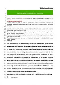
where 𝑡 ∈ [0, 20], 𝑥 ∈ [0, 1] and 𝜖1 = 10−4 , 𝜖2 = 10−6 , 𝜂 = 0.024, and 𝜃 = 0.06. The initial-boundary condition for (26) is chosen as 1 𝑢 (0, 𝑥) = 1 − (sin (3𝜋𝑥))100 , 2 1 V (0, 𝑥) = (sin (3𝜋𝑥))100 , (27) 4 𝑢 (𝑡, 1) = 𝑢 (𝑡, 0) = 1, V (𝑡, 1) = V (𝑡, 0) = 0. With these conditions, we expect three pulses in the solutions of (26). Figure 3 shows a typical behaviour of the solutions. The PDE system (26) is first discretized spatially as 𝑢𝑥𝑥 ≈ (𝑢𝑗+1 − 2𝑢𝑗 + 𝑢𝑗−1 )/Δ𝑥2 and V𝑥𝑥 ≈ (V𝑗+1 − 2V𝑗 + V𝑗−1 )/Δ𝑥2 with

Δ𝑥 = 0.01, 𝑗 = 1, 2, . . . , 100, and then a nonlinear ordinary differential system that consists of 200 ODEs is solved by the parareal algorithm. We use the IMEX Euler method to define both the GΔ𝑇 propagator and FΔ𝑡 propagator. We consider here 𝑀 = 50, Δ𝑇 = 1/10, and Δ𝑡 = Δ𝑇/𝑀. In Figure 4, we show the first 6 iterations of the parareal PIMEX-EX algorithm, where we see that the error diminishing for the solutions 𝑢 and V is very rapid. We also test the convergence speed of the parareal PIMEX-EX algorithm and the parareal algorithm which is denoted by PEX-IMEX with propagators GΔ𝑇 and FΔ𝑡 being defined by the explicit Euler and the IMEX Euler methods, respectively. The convergence curves corresponding to these three parareal algorithms are shown in Figure 5(a). We see that the PEX-IMEX algorithm is not convergent and both the other two algorithms converge rapidly. This obversion can be explained by the stability region shown in Figure 5(b), where we see that the stability region of PEX-IMEX is significantly smaller than that of the other two algorithms. Moreover, as has been shown in Figure 1, we see that the stability region of the PIMEX-EX algorithm is nearly contained in the one of PIMEX-IMEX . This means that, for the Gray-Scott model (26)-(27), if the PIMEX-EX algorithm converges, so does the PIMEX-IMEX algorithm. Moreover, it is interesting that the PIMEX-EX algorithm converges a little sharper than PIMEX-IMEX ; see Figure 5(a).

Conflict of Interests The authors declare that there is no conflict of interests regarding the publication of this paper.

Mathematical Problems in Engineering

11

Acknowledgments The authors are very grateful to the anonymous referees for the careful reading of a preliminary version of the paper and their valuable suggestions and comments, which really improve the quality of this paper. This work was supported by Science & Technology Bureau of Sichuan Province (2014JQ0035), Non-Destructive Inspection of Sichuan Institutes of Higher Education (2013QZY01), the project sponsored by OATF-UESTC, and the NSF of China (11301058, 11301362, 11371157, and 91130003).

[14]

[15]

[16]

References [1] J. Lions, Y. Maday, and G. Turinici, “A “parareal” in time discretization of PDE’s,” Comptes Rendus de I’Academie des Sciences Series I Mathematics, vol. 332, no. 1, pp. 661–668, 2001. [2] G. Bal and Y. Maday, “A “parareal” time discretization for nonlinear PDE’s with application to the pricing of an American put,” in Recent Developments in Domain Decomposition Methods, L. F. Pavarino and A. Toselli, Eds., vol. 23 of Lecture Notes in Computational Science and Engineering, pp. 189–202, 2002. [3] M. J. Gander and M. Petcu, “Analysis of a Krylov subspace enhanced parareal algorithm,” ESAIM: Proceedings, vol. 29, no. 2, pp. 556–578, 2007. [4] J. Cortial and C. Farhat, “A time-parallel implicit method for accelerating the solution of non-linear structural dynamics problems,” International Journal for Numerical Methods in Engineering, vol. 77, no. 4, pp. 451–470, 2009. [5] C. Farhat, J. Cortial, C. Dastillung, and H. Bavestrello, “Timeparallel implicit integrators for the near-real-time prediction of linear structural dynamic responses,” International Journal for Numerical Methods in Engineering, vol. 67, no. 5, pp. 697–724, 2006. [6] G. Bal, “On the convergence and the stability of the parareal algorithm to solve partial differential equations,” in Domain Decomposition Methods in Science and Engineering, vol. 40 of Lecture Notes in Computational Science and Engineering, pp. 425–432, Springer, Berlin, Germany, 2005. [7] M. J. Gander and S. Vandewalle, “Analysis of the parareal timeparallel time-integration method,” SIAM Journal on Scientific Computing, vol. 29, no. 2, pp. 556–578, 2007. [8] G. A. Staff and E. M. Rønquist, “Stability of the parareal algorithm,” in Domain Decomposition Methods in Science and Engineering, vol. 40 of Lecture Notes in Computational Science and Engineering, pp. 449–456, Springer, Berlin, Germany, 2005. [9] S. Wu, B. Shi, and C. Huang, “Parareal-Richardson algorithm for solving nonlinear ODEs and PDEs,” Communications in Computational Physics, vol. 6, no. 4, pp. 883–902, 2009. [10] M. Emmett and M. L. Minion, “Toward an efficient parallel in time method for partial differential equations,” Communications in Applied Mathematics and Computational Science, vol. 7, no. 1, pp. 105–132, 2012. [11] M. L. Minion, “A hybrid parareal spectral deferred corrections method,” Communications in Applied Mathematics and Computational Science, vol. 5, no. 2, pp. 265–301, 2010. [12] X. Dai and Y. Maday, “Stable parareal in time method for first- and second-order hyperbolic systems,” SIAM Journal on Scientific Computing, vol. 35, no. 1, pp. A52–A78, 2013. [13] L. P. He and M. X. He, “Parareal in time simulation of morphological transformation in cubic alloys with spatially

[17]

[18]

[19]

[20]

[21]

[22]

[23]

[24]

[25]

[26]

[27]

[28]

dependent composition,” Communications in Computational Physics, vol. 11, no. 5, pp. 1697–1717, 2012. C. Farhat and M. Chandesris, “Time-decomposed parallel time-integrators: theory and feasibility studies for fluid, structure, and fluid-structure applications,” International Journal for Numerical Methods in Engineering, vol. 58, no. 9, pp. 1397–1434, 2003. Y. Maday, J. Salomon, and G. Turinici, “Monotonic parareal control for quantum systems,” SIAM Journal on Numerical Analysis, vol. 45, no. 6, pp. 2468–2482, 2007. T. P. Mathew, M. Sarkis, and C. E. Schaerer, “Analysis of block parareal preconditioners for parabolic optimal control problems,” SIAM Journal on Scientific Computing, vol. 32, no. 3, pp. 1180–1200, 2010. X. Dai, C. le Bris, F. Legoll, and Y. Maday, “Symmetric parareal algorithms for Hamiltonian systems,” ESAIM: Mathematical Modelling and Numerical Analysis, vol. 47, no. 3, pp. 717–742, 2013. M. J. Gander and E. Hairer, “Analysis for parareal algorithms applied to Hamiltonian differential equations,” Journal of Computational and Applied Mathematics, vol. 259, no. part A, pp. 2– 13, 2014. J. M. Reynolds-Barredo, D. E. Newman, R. Sanchez, D. Samaddar, L. A. Berry, and W. R. Elwasif, “Mechanisms for the convergence of time-parallelized, parareal turbulent plasma simulations,” Journal of Computational Physics, vol. 231, no. 23, pp. 7851–7867, 2012. J. M. Reynolds-Barredo, D. E. Newman, and R. Sanchez, “An analytic model for the convergence of turbulent simulations time-parallelized via the parareal algorithm,” Journal of Computational Physics, vol. 255, pp. 293–315, 2013. X. Li, T. Tang, and C. Xu, “Parallel in time algorithm with spectral-subdomain enhancement for Volterra integral equations,” SIAM Journal on Numerical Analysis, vol. 51, no. 3, pp. 1735–1756, 2013. D. Guibert and D. Tromeur-Dervout, “Parallel adaptive time domain decomposition for stiff systems of ODEs/DAEs,” Computers & Structures, vol. 85, no. 9, pp. 553–562, 2007. U. M. Ascher, S. J. Ruuth, and R. J. Spiteri, “Implicit-explicit Runge-Kutta methods for time-dependent partial differential equations,” Applied Numerical Mathematics. An IMACS Journal, vol. 25, no. 2-3, pp. 151–167, 1997. S. Sekar, “Analysis of linear and nonlinear stiff problems using the RK-Butcher algorithm,” Mathematical Problems in Engineering, vol. 2006, Article ID 39246, 15 pages, 2006. U. M. Ascher, S. J. Ruuth, and B. T. Wetton, “Implicit-explicit methods for time-dependent partial differential equations,” SIAM Journal on Numerical Analysis, vol. 32, no. 3, pp. 797–823, 1995. G. J. Cooper and A. Sayfy, “Additive Runge-Kutta methods for stiff ordinary differential equations,” Mathematics of Computation, vol. 40, no. 161, pp. 207–218, 1983. M. Mechee, N. Senu, F. Ismail, B. Nikouravan, and Z. Siri, “A three-stage fifth-order Runge-Kutta method for directly solving special third-order differential equation with application to thin film flow problem,” Mathematical Problems in Engineering, vol. 2013, Article ID 795397, 7 pages, 2013. T. Koto, “IMEX Runge-Kutta schemes for reaction-diffusion equations,” Journal of Computational and Applied Mathematics, vol. 215, no. 1, pp. 182–195, 2008.

12 [29] Q. Ming, Y. Yang, and Y. Fang, “An optimized Runge-Kutta method for the numerical solution of the radial Schr¨odinger equation,” Mathematical Problems in Engineering, vol. 2012, Article ID 867948, 12 pages, 2012. [30] H. Liu and J. Zou, “Some new additive Runge-Kutta methods and their applications,” Journal of Computational and Applied Mathematics, vol. 190, no. 1-2, pp. 74–98, 2006. [31] X. Duan, J. Leng, C. Cattani, and C. Li, “A Shannon-RungeKutta-Gill method for convection-diffusion equations,” Mathematical Problems in Engineering, vol. 2013, Article ID 163734, 5 pages, 2013. [32] L. Pareschi and G. Russo, “Implicit-Explicit Runge-Kutta schemes and applications to hyperbolic systems with relaxation,” Journal of Scientific Computing, vol. 25, no. 1-2, pp. 129– 155, 2005. [33] H. Yuan, C. Song, and P. Wang, “Nonlinear stability and convergence of two-step Runge-Kutta methods for neutral delay differential equations,” Mathematical Problems in Engineering, vol. 2013, Article ID 683137, 14 pages, 2013. [34] W. Hundsdorfer and J. Verwer, Numerical Solution of TimeDependent Advection-Diffusion-Reaction Equations, Springer, Berlin, Germany, 2003. [35] J. Frank, W. Hundsdorfer, and J. G. Verwer, “On the stability of implicit-explicit linear multistep methods,” Applied Numerical Mathematics, vol. 25, no. 2-3, pp. 193–205, 1997. [36] J. G. Verwer and B. P. Sommeijer, “An implicit-explicit RungeKutta-Chebyshev scheme for diffusion-reaction equations,” SIAM Journal on Scientific Computing, vol. 25, no. 5, pp. 1824– 1835, 2004. [37] T. Koto, “Stability of IMEX Runge-Kutta methods for delay differential equations,” Journal of Computational and Applied Mathematics, vol. 211, no. 2, pp. 201–212, 2008. [38] J. E. Pearson, “Complex patterns in a simple system,” Science, vol. 261, no. 5118, pp. 189–192, 1993. [39] K. J. Lee, W. D. McCormick, Q. Ouyang, and H. L. Swinney, “Pattern formation by interacting chemical fronts,” Science, vol. 261, no. 5118, pp. 192–194, 1993.

Mathematical Problems in Engineering

Advances in

Operations Research Hindawi Publishing Corporation http://www.hindawi.com

Volume 2014

Advances in

Decision Sciences Hindawi Publishing Corporation http://www.hindawi.com

Volume 2014

Journal of

Applied Mathematics

Algebra

Hindawi Publishing Corporation http://www.hindawi.com

Hindawi Publishing Corporation http://www.hindawi.com

Volume 2014

Journal of

Probability and Statistics Volume 2014

The Scientific World Journal Hindawi Publishing Corporation http://www.hindawi.com

Hindawi Publishing Corporation http://www.hindawi.com

Volume 2014

International Journal of

Differential Equations Hindawi Publishing Corporation http://www.hindawi.com

Volume 2014

Volume 2014

Submit your manuscripts at http://www.hindawi.com International Journal of

Advances in

Combinatorics Hindawi Publishing Corporation http://www.hindawi.com

Mathematical Physics Hindawi Publishing Corporation http://www.hindawi.com

Volume 2014

Journal of

Complex Analysis Hindawi Publishing Corporation http://www.hindawi.com

Volume 2014

International Journal of Mathematics and Mathematical Sciences

Mathematical Problems in Engineering

Journal of

Mathematics Hindawi Publishing Corporation http://www.hindawi.com

Volume 2014

Hindawi Publishing Corporation http://www.hindawi.com

Volume 2014

Volume 2014

Hindawi Publishing Corporation http://www.hindawi.com

Volume 2014

Discrete Mathematics

Journal of

Volume 2014

Hindawi Publishing Corporation http://www.hindawi.com

Discrete Dynamics in Nature and Society

Journal of

Function Spaces Hindawi Publishing Corporation http://www.hindawi.com

Abstract and Applied Analysis

Volume 2014

Hindawi Publishing Corporation http://www.hindawi.com

Volume 2014

Hindawi Publishing Corporation http://www.hindawi.com

Volume 2014

International Journal of

Journal of

Stochastic Analysis

Optimization

Hindawi Publishing Corporation http://www.hindawi.com

Hindawi Publishing Corporation http://www.hindawi.com

Volume 2014

Volume 2014