Research Article Soft Sensor Model Based on Improved Elman Neural

Hindawi Journal of Sensors Volume 2018, Article ID 2981428, 10 pages https://doi.org/10.1155/2018/2981428

Research Article Soft Sensor Model Based on Improved Elman Neural Network with Variable Data Preprocessing and Its Application Hai-bo Zhu

and Yong Zhang

School of Electronics and Information Engineering, University of Science and Technology Liaoning, Anshan 114051, China Correspondence should be addressed to Yong Zhang; [email protected] Received 2 September 2018; Accepted 14 November 2018; Published 13 December 2018 Academic Editor: Jesús Lozano Copyright © 2018 Hai-bo Zhu and Yong Zhang. This is an open access article distributed under the Creative Commons Attribution License, which permits unrestricted use, distribution, and reproduction in any medium, provided the original work is properly cited. In order to solve the problems of strong coupling, nonlinearity, and complex mechanism in real-world engineering process, building soft sensor with excellent performance and robustness has become the core issue in industrial processes. In this paper, we propose a new soft sensor model based on improved Elman neural network (Elman NN) and introduce variable data preprocessing method to the soft sensor model. The improved Elman NN employs local feedback and feedforward network mechanism through context layer to accurately reflect the dynamic characteristics of the soft sensor model, which has the superiority to approximate delay systems and adaption of time-varying characteristics. The proposed variable data preprocessing method adopts combining Isometric Mapping (ISOMAP) with local linear embedding (LLE), which effectively maintains the neighborhood structure and the global mutual distance of dataset to remove the noises and data redundancy. The soft sensor model based on improved Elman NN with variable data preprocessing method by combining ISOMAP and LLE is applied in practical sintering and pelletizing to estimate the temperature in the rotary kiln calcining process. Comparing several conventional soft sensor model methods, the results indicate that the proposed method has more excellent generalization performance and robustness. Its model prediction accuracy and anti-interference ability have been improved, which provide an effective and promising method for the industrial process application.

1. Introduction Soft sensor is an inferential prediction virtual technique which adopts easily measured variables to predict the process variables which are difficult to measure directly because of technological and economical limitations or complex environment. The soft sensor tries to establish a regression prediction model between easily measured variables and difficultly measured variables, which is adopted to solve the problem that prevents the measurements from being employed as feedback signals for quality control systems. And the soft sensor methods have been employed more widely in the industrial process and become a major developing trend in both academia and industry [1]. In view of the model prediction in the industrial production process, early scholars put forward some model

predictive control, such as generalized predictive control [2, 3], dynamic matrix predictive control [4], and model algorithm control [5]. However, these soft sensor prediction methods suffer from common shortcomings. One is that the prediction control of nonlinear systems cannot be effectively solved. Another is that the stability and robustness of multivariable predictive control algorithm need to be solved and it is very difficult to build accurate principle models for complex processes. At present, with the deep research of soft sensor control theory and the continuous progress of engineering technology, some artificial intelligence and machine learning methods based on data-driven technologies are proposed to solve the problems which are difficult to measure key process and quality variables for soft sensor models, such as artificial neural network (ANN) [6–8], rough set [9], partial least squares [10], support vector machine

2 (SVM) [11–13], and hybrid methods [14, 15]. Some new works on advanced predictive control based on neural networks are referred to, for example, Ławryńczuk proposed MPC algorithms based on double-layer perceptron neural models [16]. And these data-driven soft sensors have been implemented successfully in many industrial application fields, like chemical and metallurgical engineering industries. However, the complexity of the industrial model will increase and bring about the problem of dimensionality with variables increasing. In addition, there are strong correlations and considerable redundancy between variable data. And the collected variable data may be contaminated by random noises or abnormal working condition data, which indicates that the process variables for soft sensor are stochastic. If those variable data samples are used directly for establishing the soft sensor model, the performance of the soft sensor model may not be guaranteed, which results in terrible prediction accuracy or poor estimation. Hence, it is significant to discover the general trends of data by latent variable models before soft sensor modeling. And the randomness of variable sample data should be taken into consideration and the redundant variable sample data need to be discarded selectively through the use of appropriate variable selection techniques. The core is to exploit the essential information behind the effective sample data to establish a soft sensor model that has excellent performance and strong robustness. The shortcoming of variable sample data has advanced the development of the dimension reduction methods. So many data preprocessing methods for the soft sensor model have been researched in recent years. Sun et al. [17] presented the principal component analysis (PCA) method to analyze the correlation of input variables, which is effective to reduce the dimensions of input variables from the chemical oxygen demand prediction model based on LS-SVM. Najafi et al. [18] proposed a new method called “PathBased Isomap” to find the low-dimensional embedding. The low-dimensional embedding is computed by exploiting geodesic path-mapping algorithm. Besides, some manifold learning methods have been proposed including Laplacian eigenmaps [19, 20], locally linear embedding [21], and Isometric Mapping method [22, 23]. However, these linear and nonlinear data preprocessing methods have their own limitations, which can only maintain a single feature of the variable dataset and cannot take into account other valuable characteristics. In order to overcome this problem, a data preprocessing method based on combining Isometric Mapping (ISOMAP) with local linear embedding (LLE) for input variable dataset is proposed. Hence, this paper establishes a soft sensor model based on improved Elman NN with input variable data preprocessing method which integrates ISOMAP with LLE under the kernel framework to estimate the quality variable and makes it have better performance and robustness. The rest of this paper is organized as follows. Section 2 describes the improved Elman NN and data preprocessing method. Section 3 proposes a soft sensor model based on improved Elman NN with variable data selection method by combining ISOMAP with LLE and describes it in detail. In Section 4, an industrial case study on the prediction of

Journal of Sensors y(t) . . .

Output nodes W2 . . .

W4

. . . 𝛼

W3 Context nodes Input nodes

Hidden nodes W1 . . .

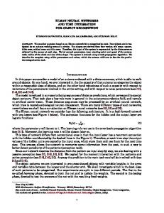
Figure 1: Architecture of improved Elman NN.

temperature in a rotary kiln calcining process in pellet sintering is given. Finally, conclusions are made in Section 5.

2. Background Theory For convenience, some definitions that will be used throughout this paper are given: NN: neural network; ISOMAP: Isometric Mapping; LLE: local linear embedding. 2.1. Improved Elman Neural Network. Elman neural network (Elman NN) [24–27] is a typical dynamic neural network with recurrent feedback layer based on BP neural network. The Elman NN stores the internal state through the context layer, which has the performance of mapping dynamic characteristics. The self-connected mode makes it sensitive to the value of the historical state and it has better ability to approximate nonlinear mapping than the BP NN. However, this feedback only aims at the hidden layer to adjust the connection weights of the internal feedback, which lacks the ability of global adjustment and dynamic stability. And the learning identification ability has some limitations. To further improve the dynamic performance and nonlinear approximation capability of Elman NN, the output of context layer as a feedback signal should be fully taken advantage of. Figure 1 shows the architecture of the improved Elman NN that is consisted of an input layer, an output layer, a hidden layer, and a context layer which is connected to hidden layer neurons and output layer neurons. From Figure 1 we can see that the improved Elman NN adds input signal from context layer nodes to the output layer, which are connected through a novel connection weight matrix W ij 4 between the context layer and output layer. After the hidden layer process, the output of the hidden layer returns to the context layer, then the intermediate state value of the context layer is transmitted to the output layer and hidden layer through the connection weight matrices W ij 4 and W ij 3 separately, which constitutes a feedforward and local feedback network. The feedback loop is formed in the hidden layer and context layer, and the path of feedforward is consisted of the input layer, hidden layer, context layer, and output layer, as shown in Figure 2.

Journal of Sensors u(Ti)

Input layer

3 W1

W3

Hidden x(Ti) W2 Output layer layer Z−1 W4 Context layer

y(Ti)

A novel set of parameter vector of the improved Elman NN can be obtained and optimized to minimize the expected average squared error: θ∗ , θ′∗ = arg min θ,θ′

Figure 2: Structure block diagram of improved Elman NN.

We define the following symbols: the number of input layer nodes, output layer nodes, and hidden layer nodes is m, n, and l, respectively. The network consisted of input data u, intermediate state oh, and response output y. The activation function of structure from the input layer to the hidden layer and from the hidden layer to the output layer is defined f θ and gθ , respectively. The mathematical model in which the input layer is mapped to the hidden layer through the mapping activation function is m

m

i=1

i=1

oh j k = f θ ui k = s 〠 w1i, j ui k + 〠 w3i, j oc j k + bhj , 1 where s represents the sigmoid function. Equation (1) is parameterized through θ = w1ij , w3ij , bhj , in which w1ij is the weight of input layer node i to the hidden layer node j; w3ij is the weight of context layer node i to the hidden layer node j and bhj is the bias vector of the hidden layer. The hidden layer oh j is mapped to the output space, y is the output vector of oh j , and the activation function is n

l

i=1

i=1

y = gθ oh j , oci = 〠 w2ij oh j k + 〠 w4ij oci k + bo

2

Equation (2) is decided by θ′ = w2ij , w4ij , bo , where is the weight of latent layer node i to the output layer node j; w4ij is the connection weight of context layer node i to the output layer node j and bo represents the bias vector of the output layer. In the training process, the output of the context layer oci k is the sum of output of the hidden layer oh j k − 1 and α times output of context layer at a previous time. w2ij

oci k = oh j k − 1 + α ⋅ oci k − 1

3

The loss function is defined as the squared error: L yd , y = y d k − y k

2

,

4

where yd k is the predicted output value at time k; yi k is the actual output value at time k.

1 n 〠 L y d ,i k , y i k n i=1

1 n = arg min 〠 L gθ′ f θ ui k n i=1 θ,θ′

5 , yi k

2.2. Input Variable Data Selection and Dimension Reduction Method. Considering the original input variables of improved Elman NN exist with redundant variable data and abnormal condition variable data, a novel variable data selection methodology by integrating Isometric Mapping (ISOMAP) [28] and local linear embedding (LLE) [29, 30] is proposed to handle measurement uncertainty and determine the dimensionality of the latent variable. The purpose is to combine two manifold learning algorithms effectively under the kernel framework and maintain various characteristics of data set, which establishes a dimensionality reduction method based on manifold learning for high-dimensional nonlinear data sets to effectively solve the network topology and the complex training problems caused by the oversize input vector data. The novel methodology can be divided into three stages. At the first stage, we construct the Mercer kernel matrix K ISOMAP of Isomap. Second, we extract the kernel matrix K LLE of LLE. At the third stage, we obtain the kernel matrix K ISOMAP−LLE under the kernel framework. The general steps of the data dimensionality reduction process are the following. Step 1. Use K neighborhood method or ε radius method to find neighborhood values. Step 2. Use the shortest path method to calculate the geodesic distance dij and to form the geodesic distance matrix D2 , in which D2ij = d 2ij ∈ RN×N . The matrix K D2 is constructed on the basis of approximate geodesic distance matrix D2 . 1 K D2 = − HD2 H, 2

6

where H represents a centralization matrix, H = I − 1/N eeT and e = 1 1 ⋯ 1 T ∈ RN×1 . Step 3. The matrix expression is constructed according to the matrix K D2 . 0

2K D2

−1

−4K D

7

Step 4. Obtain the maximum eigenvalue c∗ of the matrix and construct the Mercer kernel matrix K ISOMAP according to the maximum eigenvalue c∗ .

4

Journal of Sensors K ISOMAP = K D2 + 2cK D +

1 2 cH 2

y(t)

8

. . .

Output nodes

In order to ensure that K ISOMAP is a real symmetric semidefinite matrix, we need to satisfy c ≥ c∗ . Step 5. For each data point of the LLE algorithm xi i = 1, 2,

W2 . . .

W4

Hidden nodes

2

… , N , solve its cost function ε = xi − ∑kj=1 wij xij . The weight coefficient W ij of data points is determined, and the weight matrix W is constructed. At the same time, a real symmetric semipositive definite matrix M is obtained based on the weight matrix W, and the kernel matrix K LLE of the LLE algorithm is extracted. M= I−W

T

I−W ,

K LLE = λmax I − M,

W3 Context nodes

. . . 𝛼

. . . Input nodes

Discarded sample Training sample

9 10

W1

. . . u(Ti − 1) u(Ti) u(Ti + 1)

. . .

u(Ti + 1)

u(Ti + 2−1)

Figure 3: The structure of the soft sensor model based on improved Elman NN with dimension-reduction.

where λmax is the largest eigenvalue of the weight matrix W. Step 6. Obtain the kernel matrix of K ISOMAP‐LLE by the kernel matrix K ISOMAP of the ISOMAP algorithm and the kernel matrix K LLE of the LLE algorithm. And the kernel matrix regulator β is introduced to adjust the weight of the ISOMAP and LLE algorithms, and a new kernel matrix K ISOMAP‐LLE is constructed based on the kernel function. K ISOMAP‐LLE = K ISOMAP + 1 − β K LLE

11

Step 7. Calculate the eigenvalue matrix P and eigenvector matrix Q of the new kernel matrix K ISOMAP‐LLE and obtain the low-dimensional embedded coordinates Y based on MDS: Y = Λ1/2 Q,

12

where Λ is the diagonal matrix of P.

3. Soft Sensor Model Based on Improved Elman NN with Dimension-Reduction 3.1. Soft Sensor Model Based on Improved Elman NN with Variable Data Preprocessing. Soft sensor model based on improved Elman NN with variable data selection is aimed at exploiting the essential information behind the process data and filter redundant variable data in the soft sensor model. This paper proposes an input variable data selection and dimension-reduction methodology by integrating ISOMAP and LLE manifold learning algorithm, which is effective to solve redundant variable data and abnormal working data of the oversized sample data. This structure of the soft sensor model based on improved Elman NN with variable data selection is shown in Figure 3. The soft sensor model consisted of two parts: an input data selection (ISOMAP and LLE) and a supervised learning (improved Elman NN). In this paper, the variable screening method adopted the manifold learning variable selection method based on the

fusion of LLE and ISOMAP under the kernel framework, which is mainly reflected in two aspects. (1) The initial input variables should be chosen reasonably to make the “quality” of initial input variables be ensured. (2) The useful information of input variables should not be prematurely eliminated. And adopting supervised criterion trains each layer to obtain the weights which are set as the initial weights instead of the random initial weights. In Figure 3, W 1 , W 2 , W 3 , and W 4 are the weights of improved Elman NN, respectively, which are adopted as the weights of corresponding layers in the improved Elman NN optimized with respect to a supervised training criterion. The input data of the soft sensor model consisted of training sample data and discarded sample data: the discarded sample data U discard , i.e., noise and redundant values of the primary input variables, and the training sample data (U train , Y), i.e., pairs of input-output sample data without redundant and abnormal working data, are used to train improved Elman NN to have better accuracy for the soft sensor model. 3.2. The Training Based on Supervised Learning. In the training process of improved Elman NN, each layer in the feedforward path is considered as one-layer BP network which can update weight parameters by gradient descent. The representation of ith hidden layer is regarded as the input for the i + 1 th context layer which feeds the previous time state of the hidden layer nodes back to the hidden layer. The error is adopted to refresh the weights. The loss function can be the traditional squared error as in equation (4). Equation (5) can be reformulated by optimizing the parameters to minimize the average squared error. The gradient descent method is used to update parameters of the improved Elman NN and amend the weights wi, j 1 , wi, j 2 , wi, j 3 , and wi, j 4 to achieve self-adaptive learning. At time k, we can get T

m

Δw1ij = η1 〠 〠 yd,i k − yi k w2ij k f ′ ⋅ ⋅ ui k , k=1 i=1

13

Journal of Sensors

5

where ui k , i = 1, 2, … , m, is the signal of input layer nodes. k, k = 1, 2, … , T, is the current operation iterations. η1 is the learning rate of the weights of wi, j 1 . T

Table 1: Candidate variables of the soft sensor model for temperature prediction in the rotary kiln calcining process. Variables

n

Δw2ij = η2 〠 〠 yd,i k − yi k oh j k ,

14

k=1 i=1

where η2 is the learning rate of the weights of wi, j 2 . Δw3ij = η3

∂L ∂ohi k ∂L ∂oci k + 1 ⋅ ⋅ + 3 ∂ohi k ∂wij k ∂oci k + 1 ∂w3ij k l

〠 y d ,i k − y i k

= η3

w2ij

k f ′ ⋅ oci k

+ 〠 y d ,i k + 1 − y i k + 1

w4ij

k + 1 f ′ ⋅ oci k

i=1

,

Unit

u1

The speed of the chain grate

m/min

u2

The speed of the rotary kiln

rin/min

u3

The speed of the ring refrigerator

m/min

u4

The temperature of rotary kiln head

°

C

u5

The temperature of rotary kiln tail

°

C

u6

The quantity of coal injection I section temperature of the cooler

C

II section temperature of the cooler

°

C

u8 u9

Material thickness in the chain grate

u10

Preheating I section temperature of the smoke hood in chain grate Preheating II section temperature of the smoke hood in chain grate

u11

t °

u7

i=1 l

Description

mm °

C

°

C

15 where η3 is the learning rate of the weights of wi, j 3 . oci is obtained as in equation (3). T

n

Δw4ij = η4 〠 〠 yd,i k − yi k oci k ,

16

observational number of the soft sensor model. m is the number of selected variables through integrating ISOMAP and LLE. The optimal parameters can be obtained by the minimization of the average BIC values:

k=1 i=1

where η4 is the learning rate of the weights of wi, j 4 . A new set of weights W ij can be updated by k k+1 wk+1 ij = wij + Δwij

θ∗ , θ′∗ = arg min

y =g θ∗ ,θ′∗

〠 w2ij f i=1

m

〠 w1i, j ui i=1

〠 w3i, j oci i=1

k

The procedure of the soft sensor model based on improved Elman NN with selected variable and dimensionreduction is summarized as follows. Step 1. Initialization. Train a new improved Elman NN by the training dataset and obtain initial weight parameters of the network.

l

k +

20

17

Then, the prediction model of y is obtained by the new weight parameters θ∗ , θ′∗ . n

1 N 〠 BIC θ, θ′ N n=1

+ bhj

l

Step 2. Selection of input variable dataset.

+ 〠 w4ij oci k + bo i=1

18 3.3. Formulated the Criterion of Evaluating. After the variable selection and training, the prediction value of the soft sensor model based on improved Elman NN as in equation (18) needs be further evaluated. In this paper, the evaluation criterion, the Bayesian information criterion (BIC), is adopted as a measure between the complexity of the soft sensor model and the accuracy. BIC = n ⋅ loge

θ ∗ ,θ ′ ∗

1 n 〠 y −y 2 i=1 i i

2

+ m ⋅ loge n,

Step 2.1. Initialize variable data preprocessing method based on combining ISOMAP with LLE. Step 2.2. For the current variable dataset, calculate approximate geodesic distance to obtain the maximum eigenvalue c∗ of the matrix and construct the Mercer kernel matrix K ISOMAP by equation (8). Step 2.3. Obtain the real symmetric semipositive definite matrix M according to cost function ε and extract the kernel matrix K LLE by equation (10).

19

where yi is the prediction value by modified weight parameters as in equation (18). y is the actual value. n represents the

Step 2.4. Calculate K ISOMAP−LLE by equation (11) based on Step 2.2 and Step 2.3. Step 2.5. Calculate Y by equation (12).

6

Journal of Sensors Direct measurement variable Rotary kiln system

Principal variable (the temperature of calcining zone)

Process input variable … Secondary variable selection and data dimension reduction based on KISOMAP– LLE

Improved Elman neural networks

Predicted value + −

Bayesian optimization criterion

Figure 4: The diagram of temperature prediction in the rotary kiln calcining process based on improved Elman NN with variable data preprocessing.

Step 2.6. Obtain the input variable data without redundancy and noises disturbing. Step 3. Evaluate the parameter optimization by equation (19) and obtain the new parameters by equations (5) and (20). Step 4. Update the weight parameters by equation (17) and obtain novel neural network by equation (18).

4. Case Study: Application to Temperature Prediction in Rotary Kiln Calcining Process The rotary kiln is an important part of pellet sintering. Green pellets with a diameter of 9~16 mm are generated in the pellet making system. Then the pellets pass through the kiln tail into the rotary kiln after preheating at the chain grate. In the rotary kiln, the oxidizing roast and consolidation process of pellets is completed, which makes pellets have the physical and chemical properties of the blast furnace burden. To ensure and improve the product quality of pellets, the realtime control of temperature in the rotary kiln calcining process is very important. And the temperature in the rotary kiln calcining process is directly related to production efficiency, energy consumption, and emissions of harmful gas. By the analysis of the heat balance mechanism and technological characteristics of the rotary kiln calcining process, the temperature in the rotary kiln calcining process is coupled with multiple technological index variables in the grate system and ring cooler system, which makes it very difficult to use the instrument directly to measure the temperature in the rotary kiln calcining process because of poor working conditions or high maintenance costs of hardware sensors. Thus, the soft sensor model based on improved Elman NN with variable data selected and Bayesian optimization is applied to estimate the temperature in the rotary kiln calcining process. For the prediction of the temperature, we use the technological index variables which are correlated with prediction temperature and are easy to measure as the

input variables of the soft sensor model in this process, which are listed in Table 1. Besides, a kind of physical and chemical reactions in the rotary kiln calcining process also affect the calcining temperature. A more detailed physico-chemical mechanism of the sintering process is described in literature [31, 32]. 4.1. The Soft Sensor Model of Temperature in Rotary Kiln Calcining Process Based on Improved Elman NN with Variable Data Preprocessing. According to the technological characteristics of the rotary kiln and technology analysis, the secondary variables are selected based on the combining of ISOMAP with LLE through kernel function, which can simplify the redundant and abnormal data of the selected variables. The secondary variables are chosen as input of the soft sensor model based on improved Elman NN to predict the temperature in the rotary kiln calcining process. The Bayesian optimization criterion is applied to estimate the accuracy of prediction model and adjust the weights in order to amend the error. The structure diagram of temperature prediction in the rotary kiln calcining process based on improved Elman NN with variable data preprocessing is shown in Figure 4. 4.2. Results and Discussion. For the improved Elman NN training, data samples have been collected and are partitioned into two parts, in which 3000 process datasets of the secondary variables and corresponding temperature in the rotary kiln calcining process are selected for training, and the 1500 process datasets are applied as the testing dataset. At the same time, the data preprocessing method based on the combination of ISOMAP with LLE is used to remove the noise and data redundancy that exist in input data in order to improve prediction performance. Considering that SVM is a state-of-the-art soft sensor model with good generalization ability, the improved Elman NN with variable dataset preprocessing based on ISOMAP and LLE is compared with the soft sensor model based on SVM. The kernel

7 Prediction temperature values

Journal of Sensors 1280 1260 1240 1220

0

10

20

30

40 50 60 Sample sequence

70

80

90

100

SVM Elman NN Real values Prediction temperature error

(a) Prediction curve of the kiln burning zone temperature

10 5 0 −5

0

10

20

30

40 50 60 Sample sequence

70

80

90

100

Elman NN–error SVM–error (b) Error curve of the kiln burning zone prediction temperature

Prediction temperature values

Figure 5: Comparison of temperature generalization test in rotary kiln between Elman NN and SVM. 1280 1260 1240 1220

0

10

20

30

40 50 60 Sample sequence

70

80

90

100

Improved Elman NN SVM Real values Prediction temperature errors

(a) Prediction curve of the kiln burning zone temperature

5

0

−5

0

10

20

30

40 50 60 Sample sequence

70

80

90

100

Improved Elman NN–error SVM–error (b) Error curve of the kiln burning zone prediction temperature

Figure 6: Comparison of temperature generalization test in rotary kiln between SVM and improved Elman NN.

Journal of Sensors Prediction temperature values

8 1280

1260

1240

1220 0

10

20

30

40

50

60

70

80

90

100

80

90

100

Sample sequence Improved Elman NN with ISOMAP and LLE Improved Elman NN Real values

Prediction temperature values

(a) Prediction curve of the kiln burning zone temperature

5

0 −5 −10 0

10

20

30

40

50

60

70

Sample sequence Improved Elman NN–error Improved Elman NN with ISOMAP and LLE–error (b) Error curve of the kiln burning zone prediction temperature

Figure 7: Comparison of temperature generalization test in rotary kiln between improved Elman NN and improved Elman NN with ISOMAP and LLE.

function of SVM is the radial basis kernel function and the number of support vectors in the SVM is specified as 6. In addition, for a fair comparison, the number of hidden nodes and context nodes is the same in the Elman NN and improved Elman NN. And the number of hidden nodes is set to 36. In the improved Elman NN with data preprocessing experiments, the gradient descent is employed to train the improved Elman NN. The datasets are chosen by the ISOMAP and LLE method. In addition, the parameters are optimized and decided by comparing validation error curves according to Bayesian criterion. Once the weight parameters are fine-tuned, all training data are employed to train the model again. And the learning rate according to the loss’s change is adopted to obtain an excellent performance. To test the prediction performance of the soft sensor model based on different model methods, 100 testing samples are shown in Figures 5–7 because of that the testing datasets are too large to show. To evaluate the performance of the soft sensor model, the root mean square error (RMSE), the maximum negative error (MNE), and the maximum positive error (MPE) are typically used. The values of the testing dataset calculated through the different soft sensor models are compared in Table 2.

Table 2: Performance comparison results of prediction temperature under different soft sensor models. Soft sensor model

RMSE

MNE

MPE

Elman NN SVM Improved Elman NN Improved Elman NN with variable data preprocessing

3.0496 2.1471 1.3003

−4.582 −4.332 −3.535

5.697 3.719 3.061

0.5450

−1.275

1.941

Table 2 shows that improved Elman NN with variable data preprocessing has more excellent learning performance than other soft sensor models. The learning ability of improved Elman NN is improved to some extent and the proposed variable data preprocessing method is effective to remove the redundant data and noises. Figures 5 and 6 demonstrate that the improved Elman NN has good performance in predicting the temperature in the rotary kiln calcining process. The soft sensor model based on improved Elman NN has much better generalization and learning performance than the soft sensor model based on SVM and conventional Elman NN. The error curves of the SVM prediction, traditional Elman NN prediction, and improved Elman NN prediction which are shown in

Journal of Sensors Figures 5(b) and 6(b) clearly indicate the difference between the different methods. It can be seen that the prediction error from the improved Elman NN is smaller than that from the SVM and conventional Elman NN. However, the three methods are limited to handle the noises and data redundancy which exist in input variable data to improve the prediction performance. The soft sensor model based on improved Elman NN with ISOMAP and LLE is able to remove abnormal working condition noise and data redundancy, as shown in Figure 7. It is seen that when several abnormal noise data are added in the early stage, the improved Elman NN with ISOMAP and LLE can effectively avoid disturbance which is from noise. The improved Elman NN prediction is smooth without large fluctuations and shows better robustness than SVM prediction and improved Elman NN prediction.

5. Conclusion This paper develops a soft sensor model based on improved Elman NN and proposes a data preprocessing method based on ISOMAP and LLE for input variable data selection. The improved Elman NN introduces local feedback and feedforward networks into the Elman NN, which is trained to obtain better generalization and avoid overfitting to a certain extent. The data preprocessing method based on ISOMAP and LLE effectively keeps the neighborhood structure and the global mutual distance of the datasets and better reflects the real character of the original datasets, which is used to remove the abnormal working condition data, noises, and data redundancy in the input variables from improved Elman NN. The soft sensor model based on improved Elman NN with data preprocessing by ISOMAP and LLE is applied to estimate the temperature in the rotary kiln calcining process. The prediction values of the soft sensor model based on improved Elman NN with data preprocessing through ISOMAP and LLE follow the varying trend of the temperature very effectively and have excellent robustness and generalization performance. The great performance illustrates that the soft sensor model based on improved Elman NN with data preprocessing through ISOMAP and LLE provides a powerful and promising method for complex industrial process applications.

Data Availability The prediction temperature of the rotary kiln calcining process in Sintering and Pelletizing data used to support the findings of this study have not been made available because the data which is used is the proprietary data from a Sintering and Pelletizing company that will share the data only with regulatory agencies but not with researchers. So the jurisdiction of the data is limited.

Conflicts of Interest The authors declare that there is no conflict of interests regarding the publication of this paper.

9

Acknowledgments This work was supported in part by the Project by National Natural Science Foundation of China under Grant (61473054).

References [1] W. Yan, D. Tang, and Y. Lin, “A data-driven soft sensor modeling method based on deep learning and its application,” IEEE Transactions on Industrial Electronics, vol. 64, no. 5, pp. 4237–4245, 2017. [2] D. W. Clarke and C. Mohtadi, “Properties of generalized predictive control,” Automatica, vol. 25, no. 6, pp. 859–875, 1989. [3] P. Albertos and R. Ortega, “On generalized predictive control: two alternative formulations,” Automatica, vol. 25, no. 5, pp. 753–755, 1989. [4] C. R. Cutler and B. L. Ramaker, “Dynamic matrix control computer control algorithm,” Joint Automatic Control Conference, vol. 17, p. 72, 1980. [5] J. Richalet, A. Rault, J. L. Testud, and J. Papon, “Model predictive heuristic control: applications to industrial processes,” Automatica, vol. 14, no. 5, pp. 413–428, 1978. [6] D. I. Adelani and M. K. Traoré, “Enhancing the reusability and interoperability of artificial neural networks with DEVS modeling and simulation,” International Journal of Modeling, Simulation, and Scientific Computing, vol. 7, no. 2, article 1650005, 2016. [7] A. Afram, F. Janabi-Sharifi, A. S. Fung, and K. Raahemifar, “Artificial neural network (ANN) based model predictive control (MPC) and optimization of HVAC systems: a state of the art review and case study of a residential HVAC system,” Energy and Buildings, vol. 141, pp. 96–113, 2017. [8] P. Chopra, R. K. Sharma, and M. Kumar, “Prediction of compressive strength of concrete using artificial neural network and genetic programming,” Advances in Materials Science and Engineering, vol. 2016, Article ID 7648467, 10 pages, 2016. [9] Q. Cheng, Z. Qi, G. Zhang, Y. Zhao, B. Sun, and P. Gu, “Robust modelling and prediction of thermally induced positional error based on grey rough set theory and neural networks,” International Journal of Advanced Manufacturing Technology, vol. 83, no. 5–8, pp. 753–764, 2016. [10] J. Zheng and Z. Song, “Semisupervised learning for probabilistic partial least squares regression model and soft sensor application,” Journal of Process Control, vol. 64, pp. 123–131, 2018. [11] K. Y. Bae, H. S. Jang, and D. K. Sung, “Hourly solar irradiance prediction based on support vector machine and its error analysis,” IEEE Transactions on Power Systems, vol. 32, no. 2, pp. 935–945, 2017. [12] Z. Ju and H. Gu, “Predicting pupylation sites in prokaryotic proteins using semi-supervised self-training support vector machine algorithm,” Analytical Biochemistry, vol. 507, pp. 1–6, 2016. [13] L. Zago, P. Y. Hervé, R. Genuer et al., “Predicting hemispheric dominance for language production in healthy individuals using support vector machine,” Human Brain Mapping, vol. 38, no. 12, pp. 5871–5889, 2017. [14] R. Grbić, D. Slišković, and P. Kadlec, “Adaptive soft sensor for online prediction and process monitoring based on a mixture of Gaussian process models,” Computers & Chemical Engineering, vol. 58, no. 22, pp. 84–97, 2013.

10 [15] M. Zhang and X. Liu, “A soft sensor based on adaptive fuzzy neural network and support vector regression for industrial melt index prediction,” Chemometrics and Intelligent Laboratory Systems, vol. 126, no. 126, pp. 83–90, 2013. [16] M. Ławryńczuk, “Computationally efficient model predictive control algorithms,” Studies in Systems, Decision and Control, vol. 3, no. 1, pp. 137–149, 2014. [17] J. Sun, Z. Cheng, R. Yang, and S. Shan, “Soft-sensor modeling for paper mill effluent COD based on PCA-PSO-LSSVM,” Computers & Applied Chemistry, vol. 34, no. 9, pp. 706–710, 2017. [18] A. Najafi, A. Joudaki, and E. Fatemizadeh, “Nonlinear dimensionality reduction via path-based isometric mapping,” IEEE Transactions on Pattern Analysis and Machine Intelligence, vol. 38, no. 7, pp. 1452–1464, 2016. [19] J. Wang, “Laplacian Eigenmaps,” in Geometric Structure of High-Dimensional Data and Dimensionality Reduction, pp. 235–247, Springer, 2012. [20] M. Belkin and P. Niyogi, “Laplacian eigenmaps for dimensionality reduction and data representation,” Neural Computation, vol. 15, no. 6, pp. 1373–1396, 2014. [21] Y. Huang, L. Jin, H. S. Zhao, and X. Y. Huang, “Fuzzy neural network and LLE algorithm for forecasting precipitation in tropical cyclones: comparisons with interpolation method by ECMWF and stepwise regression method,” Natural Hazards, vol. 91, no. 1, pp. 201–220, 2018. [22] X. Wang, S. Chen, and M. Yao, “Data dimensionality reduction method of semi-supervised isometric mapping based on regularization,” Journal of Electronics & Information Technology, vol. 33, no. 1, pp. 241–245, 2016. [23] G. Kanishka and T. I. Eldho, “Watershed classification using Isomap technique and hydrometeorological attributes,” Journal of Hydrologic Engineering, vol. 22, no. 10, article 04017040, 2017. [24] G. Ren, Y. Cao, S. Wen, T. Huang, and Z. Zeng, “A modified Elman neural network with a new learning rate scheme,” Neurocomputing, vol. 286, pp. 11–18, 2018. [25] K. Kolanowski, A. Świetlicka, R. Kapela, J. Pochmara, and A. Rybarczyk, “Multisensor data fusion using Elman neural networks,” Applied Mathematics and Computation, vol. 319, pp. 236–244, 2018. [26] Y. Ge, Y. Huang, D. Hao, G. Li, and H. Li, “An indicated torque estimation method based on the Elman neural network for a turbocharged diesel engine,” Proceedings of the Institution of Mechanical Engineers Part D Journal of Automobile Engineering, vol. 230, no. 10, pp. 1299–1313, 2016. [27] A. Wysocki and M. Ławryńczuk, “Elman neural network for modeling and predictive control of delayed dynamic systems,” Archives of Control Sciences, vol. 26, no. 1, pp. 117–142, 2016. [28] H. Choi and S. Choi, “Robust kernel Isomap,” Pattern Recognition, vol. 40, no. 3, pp. 853–862, 2007. [29] Y. Zhang, Y. Fu, Z. Wang, and L. Feng, “Fault detection based on modified kernel semi-supervised locally linear embedding,” IEEE Access, vol. 6, pp. 479–487, 2018. [30] B. Jiang, C. Ding, and B. Luo, “Robust data representation using locally linear embedding guided PCA,” Neurocomputing, vol. 275, pp. 523–532, 2018.

Journal of Sensors [31] Y. Qianli and Q. Liyun, “A diagnosis method of rotary kiln lining based on extreme learning machine (ELM) and its application,” Sintering and Pelletizing, vol. 40, no. 6, pp. 18–22, 2015. [32] G. Zhang and J. Zhang, “A novel RS-SVM dynamic prediction approach and its application,” Process Automation Instrumentation, vol. 26, no. 2, pp. 17–20, 2005.

International Journal of

Advances in

Rotating Machinery

Engineering Journal of

Hindawi www.hindawi.com

Volume 2018

The Scientific World Journal Hindawi Publishing Corporation http://www.hindawi.com www.hindawi.com

Volume 2018 2013

Multimedia

Journal of

Sensors Hindawi www.hindawi.com

Volume 2018

Hindawi www.hindawi.com

Volume 2018

Hindawi www.hindawi.com

Volume 2018

Journal of

Control Science and Engineering

Advances in

Civil Engineering Hindawi www.hindawi.com

Hindawi www.hindawi.com

Volume 2018

Volume 2018

Submit your manuscripts at www.hindawi.com Journal of

Journal of

Electrical and Computer Engineering

Robotics Hindawi www.hindawi.com

Hindawi www.hindawi.com

Volume 2018

Volume 2018

VLSI Design Advances in OptoElectronics International Journal of

Navigation and Observation Hindawi www.hindawi.com

Volume 2018

Hindawi www.hindawi.com

Hindawi www.hindawi.com

Chemical Engineering Hindawi www.hindawi.com

Volume 2018

Volume 2018

Active and Passive Electronic Components

Antennas and Propagation Hindawi www.hindawi.com

Aerospace Engineering

Hindawi www.hindawi.com

Volume 2018

Hindawi www.hindawi.com

Volume 2018

Volume 2018

International Journal of

International Journal of

International Journal of

Modelling & Simulation in Engineering

Volume 2018

Hindawi www.hindawi.com

Volume 2018

Shock and Vibration Hindawi www.hindawi.com

Volume 2018

Advances in

Acoustics and Vibration Hindawi www.hindawi.com

Volume 2018