Research Article Solving Fuzzy Fractional Differential

Hindawi Publishing Corporation The Scientific World Journal Volume 2013, Article ID 454969, 11 pages http://dx.doi.org/10.1155/2013/454969

Research Article Solving Fuzzy Fractional Differential Equations Using Zadeh’s Extension Principle M. Z. Ahmad,1 M. K. Hasan,2 and S. Abbasbandy3 1

Institute of Engineering Mathematics, Universiti Malaysia Perlis, Kampus Tetap Pauh Putra, 02600 Arau, Perlis, Malaysia School of Information Technology, Faculty of Information Science and Technology, Universiti Kebangsaan Malaysia, 43600 Bangi, Selangor, Malaysia 3 Department of Mathematics, Imam Khomeini International University, Ghazvin 34149-16818, Iran 2

Correspondence should be addressed to M. Z. Ahmad; [email protected] Received 25 June 2013; Accepted 24 July 2013 Academic Editors: M. Bruzón and S. Momani Copyright © 2013 M. Z. Ahmad et al. This is an open access article distributed under the Creative Commons Attribution License, which permits unrestricted use, distribution, and reproduction in any medium, provided the original work is properly cited. We study a fuzzy fractional differential equation (FFDE) and present its solution using Zadeh’s extension principle. The proposed study extends the case of fuzzy differential equations of integer order. We also propose a numerical method to approximate the solution of FFDEs. To solve nonlinear problems, the proposed numerical method is then incorporated into an unconstrained optimisation technique. Several numerical examples are provided.

1. Introduction Fractional calculus is an important branch in mathematical analysis. It is a generalisation of ordinary calculus that allows noninteger order. At the beginning, it was slowly established. However, after Leibniz and Newton invented differential calculus, it has been a subject of interest among mathematicians, physicists, and engineers. Consequently, the theory of fractional calculus has been extensively developed and influenced in many areas of discipline. The fractional integral and fractional derivative of Riemann-Liouville, for example, have been applied to solve many mathematical problems [1–6]. One of the particular interests is the case of solving fractional differential equations [7–9]. The fractional derivative of Riemann-Liouville, however, has a common characteristic. It requires a quantity of fractional derivative of unknown solution at initial point. In practice, we do not clearly know what the meaning of the fractional derivative at that point is. In other words, the required quantity cannot be measured and perhaps may not be available [10, 11]. The well-known and popularly used method in solving fractional differential equations is the Caputo fractional derivative. It allows to specify a quantity of integer order derivatives at the initial point. This quantity typically is available and can be measured. It is therefore not surprising that

there is a vast literature dealing with fractional differential equations involving the Caputo fractional derivative [12–16]. The theory and application of fractional differential equations under both types of fractional derivatives have been discussed by many authors [11, 17–25]. Some potential applications have been studied in [26–28]. In the context of mathematical modelling, developing an accurate fractional differential equation is not a simple task. It requires an understanding of real physical phenomena involved. The real physical phenomena, however, are always pervaded with uncertainty. This is obvious when dealing with “living” materials such as soil, water, and microbial populations [29]. When a real physical phenomenon is modelled by a fractional differential equation, namely, 𝐷𝑎𝛽 𝑥 (𝑡) = 𝑓 (𝑡, 𝑥 (𝑡)) ,

0 < 𝛽 ≤ 1, 𝑡 > 𝑎,

𝑥 (𝑡0 ) = 𝑥0 ,

(1)

we cannot usually be sure that the model is perfect. For example, the initial value in (1) may not be known precisely. It may take any value in the form of “less than 𝑥0 ,” “about 𝑥0 ,” or “more than 𝑥0 .” Classical mathematics, however, fail to cope with this situation. Therefore, it is necessary to have other theories in order to handle this issue. Various theories

2

The Scientific World Journal

exist for describing this situation and the most popular one is the fuzzy set theory [30]. In order to obtain a more realistic model than (1), Agarwal et al. [31] have taken an initiative to introduce the concept of solution for fuzzy fractional differential equations. This contribution has motivated several authors to establish some results on the existence and uniqueness of solution (see [32]). In [33], the authors derived the explicit solution of fuzzy fractional differential equations using the Riemann-Liouville H-derivative. Recently, Salahshour et al. [34] applied fuzzy Laplace transforms [35] to solve fuzzy fractional differential equations. Basically, the proposed ideas are a generalisation of the theory and solution of fuzzy differential equations [36– 41]. However, the authors considered fuzzy fractional differential equations under the Riemann-Liouville H-derivative. Again, it requires a quantity of fractional H-derivative of an unknown solution at the fuzzy initial point. In this paper, we propose a new interpretation of fuzzy fractional differential equations and present their solutions analytically and numerically. The proposed idea is a generalisation of the interpretation given in [42–49], where the authors used Zadeh’s extension principle to interpret fuzzy differential equations. According to Mizukoshi et al. [43], this interpretation requires neither the concept of derivatives of a fuzzy function nor the use of selection theory to obtain a solution to the fuzzy differential equation. This paper is organised in the following sequence. In Section 2, we recall some basic definitions and theoretical backgrounds needed in this paper. In Section 3, we present the solution of fuzzy fractional differential equations analytically and numerically. In Section 4, some numerical examples are given. Finally in Section 5, we give conclusions.

2. Basic Concepts In this section, we briefly elaborate some definitions and important concepts of fractional calculus and fuzzy set. 2.1. The Fractional Integral and Fractional Derivative. The following definitions of fractional integral and fractional derivative are adopted from [11]. Definition 1. A real function 𝑥(𝑡), 𝑡 > 0, is said to be in the space 𝐶𝜇 , 𝜇 ∈ R, if there exists a real number 𝑝 > 𝜇, such that 𝑥(𝑡) = 𝑡𝑝 𝑥1 (𝑡), where 𝑥1 (𝑡) ∈ 𝐶(0, ∞) and it is said to be in the space 𝐶𝜇𝑛 if and only if 𝑥𝑛 ∈ 𝐶𝜇 , 𝑛 ∈ N. Definition 2. The Riemann-Liouville fractional integral of 𝑥 of order 𝛽 > 0 with 𝑎 ≥ 0 is defined as 𝐼𝑎𝛽 𝑥 (𝑡) =

𝑡 1 ∫ (𝑡 − 𝑠)𝛽−1 𝑥 (𝑠) 𝑑𝑠, Γ (𝛽) 𝑎

𝑡 > 𝑎,

(2)

and for 𝛽 = 0, the Riemann-Liouville fractional integral of 𝑥 is defined as 𝐼𝑎0 𝑥 (𝑡) = 𝑥 (𝑡) .

(3)

Here, Γ(𝛽) is the well-known gamma function defined as ∞

Γ (𝛽) = ∫ 𝑡𝛽−1 𝑒−𝑡 𝑑𝑡.

(4)

0

Definition 3. The Caputo fractional derivative of 𝑥 of order 𝛽 > 0 with 𝑎 ≥ 0 is defined as 𝑐

𝐷𝑎𝛽 𝑥 (𝑡) =

𝑡 1 ∫ (𝑡 − 𝑠)𝑛−𝛽−1 𝑥(𝑛) (𝑠) 𝑑𝑠 Γ (𝑛 − 𝛽) 𝑎

(5)

𝑛 . for 𝑛 − 1 < 𝛽 ≤ 𝑛, 𝑛 ∈ N, 𝑡 ≥ 𝑎, 𝑥 ∈ 𝐶−1

The following are two basic properties of the Caputo fractional derivative [50]. 𝑛 (1) Let 𝑥 ∈ 𝐶−1 , 𝑛 ∈ N. Then 𝑐 𝐷𝑎𝛽 𝑥, 0 ≤ 𝛽 ≤ 𝑛, is well defined and 𝑐 𝐷𝑎𝛽 𝑥 ∈ 𝐶−1 . (2) Let 𝑛 − 1 < 𝛽 ≤ 𝑛, 𝑛 ∈ N, and 𝑥 ∈ 𝐶𝜇𝑛 , 𝜇 ≥ −1. Then 𝑛−1

𝐼𝑎𝛽 ( 𝑐 𝐷𝑎𝛽 ) 𝑥 (𝑡) = 𝑥 (𝑡) − ∑ 𝑥(𝑘) (𝑎) 𝑘=0

(𝑡 − 𝑎)𝑘 . 𝑘!

(6)

The Laplace transform of the Caputo fractional derivative is given by [51] L { 𝑐 𝐷𝛽 𝑥 (𝑡)} 𝑛−1

= 𝑠𝛽 𝑋 (𝑠) − ∑ 𝑠𝛽−𝑘−1 𝑥(𝑘) (0) ;

𝑛 − 1 < 𝛽 ≤ 𝑛.

(7)

𝑘=0

2.2. Fuzzy Set Theory. According to Zadeh [30], a fuzzy set is a generalisation of a classical set that allows a membership function to take any value in the unit interval [0, 1]. Definition 4 (see [30]). Let 𝑈 be a universal set. A fuzzy set 𝐴 in 𝑈 is defined by a membership function 𝐴(𝑥) that maps every element in 𝑈 to the unit interval [0, 1]. Definition 5 (see [38]). Let 𝐴 be a fuzzy set defined in R. 𝐴 is called a fuzzy number if (i) 𝐴 is normal: there exists 𝑥0 ∈ R such that 𝐴(𝑥0 ) = 1; (ii) 𝐴 is convex: for all 𝑥, 𝑦 ∈ R and 0 ≤ 𝜆 ≤ 1, it holds that 𝐴 (𝜆𝑥 + (1 − 𝜆) 𝑦) ≥ min (𝐴 (𝑥) , 𝐴 (𝑦)) ;

(8)

(iii) 𝐴 is upper semicontinuous: for any 𝑥0 ∈ R, it holds that 𝐴 (𝑥0 ) ≥ lim± 𝐴 (𝑥) ; 𝑥 → 𝑥0

(9)

(iv) [𝐴]0 = {𝑥 ∈ R | 𝐴(𝑥) > 0} is a compact subset of R. Definition 6 (see [38]). Let 𝐴 be a fuzzy number defined in R. The 𝛼-cut of 𝐴 is the crisp set [𝐴]𝛼 that contains all elements in R such that the membership value of 𝐴 is greater than or equal to 𝛼; that is, [𝐴]𝛼 = {𝑥 ∈ 𝑈 | 𝐴 (𝑥) ≥ 𝛼} ,

𝛼 ∈ (0, 1] .

(10)


3

For a fuzzy number 𝐴, its 𝛼-cuts are closed intervals in R and we denote them by

For 𝐴, 𝐵 ∈ F(R) and 𝜆 ∈ R, the sum 𝐴 + 𝐵 and the product 𝜆𝐴 are defined as follows, respectively:

[𝐴]𝛼 = [𝑎1𝛼 , 𝑎2𝛼 ] .

[𝐴 + 𝐵]𝛼 = [𝐴]𝛼 + [𝐵]𝛼 ,

(11)

Definition 7 (see [52]). A fuzzy number 𝐴 is called a triangular fuzzy number if its membership function has the following form: 0, { { 𝑥−𝑎 { { { , { {𝑏 − 𝑎 𝐴 (𝑥) = { {𝑐 − 𝑥 { { , { {𝑐 − 𝑏 { {0,

if 𝑥 < 𝑎, if 𝑎 ≤ 𝑥 < 𝑏, (12) if 𝑏 ≤ 𝑥 ≤ 𝑐, if 𝑥 > 𝑐,

and its 𝛼-cuts are simply [𝐴]𝛼 = [𝑎 + 𝛼(𝑏 − 𝑎), 𝑐 − 𝛼(𝑐 − 𝑏)], 𝛼 ∈ (0, 1]. In this paper, we denote 𝐴 = (𝑎, 𝑏, 𝑐) as the triangular fuzzy number and F(R) as the set of all triangular fuzzy numbers. Any crisp function can be extended to take fuzzy set as arguments by applying Zadeh’s extension principle [30]. Let 𝑓 be a function from 𝑋 to 𝑌. Given a fuzzy set 𝐴 in 𝑋, we want to find a fuzzy set 𝐵 = 𝑓(𝐴) in 𝑌 that is induced by 𝑓. If 𝑓 is a strictly monotone, then we can extend 𝑓 to fuzzy set as follows: 𝐴 (𝑓−1 (𝑦)) , if 𝑦 ∈ range (𝑓) , 𝑓 (𝐴) (𝑦) = { 0, if 𝑦 ∉ range (𝑓) .

(13)

It is clear that (13) can be easily calculated by determining the membership at the endpoints of the 𝛼-cuts of 𝐴. However, in general, the process of finding the fuzzy set 𝐵 = 𝑓(𝐴) is more complicated and cannot be gathered easily. For example, if 𝑓 is nonmonotone, then the problem can arise when two or more distinct points in 𝑋 are mapped to the same point in 𝑌. If this is the case, then the above equation may take two or more different values. This requires a new extension of (13) as shown below: { sup 𝐴 (𝑥) , if 𝑦 ∈ range (𝑓) , 𝑓 (𝐴) (𝑦) = {𝑥∈𝑓−1 (𝑦) if 𝑦 ∉ range (𝑓) , {0,

[𝜆𝐵]𝛼 = 𝜆[𝐴]𝛼

(17)

for each 𝛼 ∈ [0, 1]. Definition 9 (see [56]). If 𝐴 and 𝐵 are two fuzzy numbers, then the distance 𝐷 between 𝐴 and 𝐵 is defined as 󵄨 󵄨 󵄨 󵄨 𝐷 (𝐴, 𝐵) = sup max {󵄨󵄨󵄨𝑎1𝛼 − 𝑏1𝛼 󵄨󵄨󵄨 , 󵄨󵄨󵄨𝑎2𝛼 − 𝑏2𝛼 󵄨󵄨󵄨} . (18) 𝛼∈[0,1]

In [57], the authors have shown that (F(R), 𝐷) is a complete metric space and the following properties are well known: (i) 𝐷(𝐴 + 𝐶, 𝐵 + 𝐶) = 𝐷(𝐴, 𝐵), ∀𝐴, 𝐵, 𝐶 ∈ F(R), (ii) 𝐷(𝜆𝐴, 𝜆𝐵) = |𝜆|𝐷(𝐴, 𝐵), ∀𝐴, 𝐵 ∈ F(R) and 𝜆 ∈ R, (iii) 𝐷(𝐴 + 𝐵, 𝐶 + 𝐷) ≤ 𝐷(𝐴, 𝐶) + 𝐷(𝐵, 𝐷), ∀𝐴, 𝐵, 𝐶, 𝐷 ∈ F(R).

3. Fuzzy Fractional Differential Equations In this section, we present analytical and numerical solutions of fuzzy fractional differential equations. 3.1. Analytical Solution of Fuzzy Fractional Differential Equations. First, let us consider the following fractional differential equation: 𝑐

𝐷𝑎𝛽 𝑥 (𝑡) = 𝑓 (𝑡, 𝑥 (𝑡)) , 𝑥 (𝑡0 ) = 𝑥0 ,

(19)

where 𝑓 : [𝑡0 , 𝑇] × R → R is a real-valued function, 𝑥0 ∈ R, and 𝛽 ∈ (0, 1]. If 𝛽 = 1, then (19) becomes an ordinary differential equation. Assume that the initial value is replaced by a fuzzy number; then we have the following fuzzy fractional differential equation:

(14)

𝑐

𝐷𝑎𝛽 𝑋 (𝑡) = 𝑓 (𝑡, 𝑋 (𝑡)) , 𝑋 (𝑡0 ) = 𝑋0 ,

where

(20)

Some computational methods to compute (14) can be found in [53, 54].

where 𝑋0 ∈ F(R) and 𝛽 ∈ (0, 1]. If 𝛽 = 1, then (20) becomes a fuzzy differential equation. In order to find the solution of (20), we first find the solution of (19). By taking the Laplace transform on both sides of (19), we get

Theorem 8 (see [55]). If 𝑓 : R → R is continuous, then 𝑓 : F(R) → F(R) is well defined and

L [ 𝑐 𝐷𝑎𝛽 𝑥 (𝑡)] = L [𝑓 (𝑡, 𝑥 (𝑡))] .

(21)

𝑠𝛽 L {𝑥 (𝑡)} − 𝑥 (𝑡0 ) 𝑠𝛽−1 = L [𝑓 (𝑡, 𝑥 (𝑡))] .

(22)

𝑓−1 (𝑦) = {𝑥 ∈ 𝑋 | 𝑓 (𝑥) = 𝑦} .

𝛼

[𝑓(𝐴)] = 𝑓 ([𝐴]𝛼 ) , ∀𝛼 ∈ [0, 1] , ∀𝐴 ∈ F (R) , where 𝑓(𝐴) = {𝑓(𝑢) | 𝑢 ∈ [𝐴]𝛼 }.

(15)

(16)

It follows that

4


Assume that after simplifying (22), we get

It follows that (23)

𝛼 𝛼 , 𝑥0,2 ]} , 𝑥1𝛼 (𝑡) = min {𝑔 (𝑡, 𝛽, 𝑢) | 𝑢 ∈ [𝑥0,1

Then by taking the inverse Laplace transform to (23), we have

𝛼 𝛼 , 𝑥0,2 ]} 𝑥2𝛼 (𝑡) = max {𝑔 (𝑡, 𝛽, 𝑢) | 𝑢 ∈ [𝑥0,1

L [𝑥 (𝑡)] = 𝑚 (𝑠) .

𝑥 (𝑡) = L−1 [𝑚 (𝑠)] = 𝑔 (𝑡, 𝛽, 𝑥0 ) ,

(24)

for 𝑡 ∈ [𝑡0 , 𝑇] and 𝑥0 ∈ R. In order to find the solution of (20), we fuzzify (24) using Zadeh’s extension principle. Hence, we have 𝑋 (𝑡) = 𝑔̂ (𝑡, 𝛽, 𝑋0 ) ,

(25)

which is the solution of (20). This procedure can be shown precisely in the following theorem. Theorem 10. Let 𝐺 be an open set in R and [𝑋0 ]𝛼 ∈ F(R) ⊂ 𝐺. Suppose that 𝑓 is continuous and that for each 𝛽 ∈ (0, 1] and each 𝑥0 ∈ 𝐺 there exists a unique solution 𝑔(⋅, 𝛽, 𝑥0 ) of the problem (19) and that 𝑔(𝑡, 𝛽, ⋅) is continuous in 𝐺 for each 𝑡 ∈ [𝑡0 , 𝑇] fixed. Then, there exists a unique fuzzy solution 𝑋(𝑡) = ̂ 𝛽, 𝑋0 ) of the problem (20). 𝑔(𝑡, Proof. The proof of this theorem uses the basic idea found in [46]. Since 𝑓 is continuous, there exists a unique solution 𝑔(𝑡, 𝛽, 𝑥0 ). This solution is well defined and continuous in 𝐺, for each 𝑡 ∈ [𝑡0 , 𝑇] fixed. Then, from Theorem 8, we have ̂ 𝛽, ⋅) : F(𝐺) → F(R), which is continuous and well 𝑔(𝑡, defined. Therefore, there exists a unique fuzzy solution of the ̂ 𝛽, 𝑋0 ) for the problem (20). form 𝑋(𝑡) = 𝑔(𝑡, Remark 11. The existence of 𝑋(𝑡) is guaranteed by Theorem 8 since 𝑥(𝑡) is continuous. Moreover, in order to have valid level sets, 𝑋(𝑡) should satisfy the following Staking Theorem [58]. Theorem 12. If 𝑋 : [𝑡0 , 𝑇] → F(R) is a fuzzy solution of (20) and denoting [𝑋(𝑡)]𝛼 = [𝑥1𝛼 (𝑡), 𝑥2𝛼 (𝑡)] for 𝛼 ∈ [0, 1], then 𝛼

(i) [𝑋(𝑡)] is nonempty compact subset of R; (ii) [𝑋(𝑡)]𝛼2 ⊆ [𝑋(𝑡)]𝛼1 for 0 ≤ 𝛼1 ≤ 𝛼2 ≤ 1;

𝛼𝑛 (iii) [𝑋(𝑡)]𝛼 = ⋂∞ for any nondecreasing 𝑛=1 [𝑋(𝑡)] sequence 𝛼𝑛 → 𝛼 in [0, 1].

In the following result, we will show that 𝑥1𝛼 (𝑡) and 𝑥2𝛼 (𝑡) do not interchange at all 𝑡 ∈ [𝑡0 , ∞). Theorem 13. If 𝑋(𝑡) = 𝑔(𝑡, 𝛽, 𝑋0 ) is obtained by using Theorem 10 and [𝑋(𝑡)]𝛼 = [𝑥1𝛼 (𝑡), 𝑥2𝛼 (𝑡)] for 𝛼 ∈ [0, 1], then 𝑥1𝛼 (𝑡) and 𝑥2𝛼 (𝑡) do not interchange at all 𝑡 ∈ [𝑡0 , ∞). Proof. We know that 𝑋(𝑡) is obtained by Zadeh’s extension principle through Theorem 10; then its membership function has the following form: { sup 𝑋0 (𝑥) , if 𝑦 ∈ range (𝑔) , 𝑋 (𝑡) (𝑦) = {𝑥∈𝑔−1 (𝑡,𝛽,𝑦) if 𝑦 ∉ range (𝑔) . {0,

(26)

(27)

for 𝛼 ∈ [0, 1]. It is obvious that 𝑥1𝛼 (𝑡) ≤ 𝑥2𝛼 (𝑡) .

(28)

This holds for all 𝑡 ∈ [𝑡0 , ∞). This completes the proof. In general, the solution of (20) may not be found analytically. Therefore, a numerical method must be proposed. 3.2. Numerical Solution of Fuzzy Fractional Differential Equations. Fractional Euler method under the Caputo fractional derivative has been proposed in [59]. However, in order to approximate the solution of fuzzy fractional differential equations, the fractional Euler method has to be extended in the fuzzy setting. In this case, Zadeh’s extension principle plays an important role. Let 𝑥(𝑡) be the solution of (19). The first two terms of fractional Taylor series for 𝑥(𝑡) at 𝑡𝑖 can be written as [59] 𝑥 (𝑡𝑖+1 ) ≈ 𝑥 (𝑡𝑖 ) + 𝑐 𝐷𝛽 𝑥 (𝑡𝑖 )

ℎ𝛽 . Γ (𝛽 + 1)

(29)

From (19), we have 𝑥 (𝑡𝑖+1 ) ≈ 𝑥 (𝑡𝑖 ) +

ℎ𝛽 𝑓 (𝑡𝑖 , 𝑥 (𝑡𝑖 )) . Γ (𝛽 + 1)

(30)

Let 𝑤𝑖+1 ≈ 𝑥(𝑡𝑖+1 ); then we have the following fractional Euler method [59]: 𝑤𝑖+1 = 𝑤𝑖 +

ℎ𝛽 𝑓 (𝑡𝑖 , 𝑤𝑖 ) , Γ (𝛽 + 1)

(31)

for 𝑖 = 0, 1, 2, . . . , 𝑁. Let 𝑔(𝛽, ℎ, 𝑡𝑖 , 𝑤𝑖 ) = 𝑤𝑖 + (ℎ𝛽 /Γ(𝛽 + 1))𝑓(𝑡𝑖 , 𝑤𝑖 ); then (31) becomes 𝑤𝑖+1 = 𝑔 (𝛽, ℎ, 𝑡𝑖 , 𝑤𝑖 ) .

(32)

To approximate the solution of (20), (32) will be fuzzified using Zadeh’s extension principle. We then obtain the following fuzzy fractional Euler method: 𝑊𝑖+1 = 𝑔 (𝛽, ℎ, 𝑡𝑖 , 𝑊𝑖 )

(33)

for 𝑖 = 0, 1, . . . , 𝑁, and 𝑊𝑖 ∈ F(R). Please note that if 𝛽 = 1, then this fuzzy fractional Euler method becomes fuzzy Euler method as proposed in [47]. The membership function of 𝑔 in (33) can be defined as 𝑔 (𝛽, ℎ, 𝑡𝑖 , 𝑊𝑖 ) (𝑦) 𝑊𝑖 (𝑥) , if 𝑦 ∈ range (𝑔) , sup { = {𝑥∈𝑔−1 (𝛽,ℎ,𝑡𝑖 ,𝑦) if 𝑦 ∉ range (𝑔) . {0,

(34)


5

Input: Fractional Euler Equation, Fuzzy Initial Value, 𝛽, 𝑡0 , 𝑡𝑁 and 𝑁 Descritise 𝛼 ← {𝛼0 , 𝛼1 , . . . , 𝛼𝑛 }; 𝑡 −𝑡 ℎ ← 𝑁 0; 𝑁 for 𝑗 = #(𝛼) do 𝑤1 (1, 𝑗) ← 𝑎 + 𝛼(𝑗) ∗ (𝑏 − 𝑎); 𝑤2 (1, 𝑗) ← 𝑐 − 𝛼(𝑗) ∗ (𝑐 − 𝑏); end for 𝑖 = 1 : 𝑁 do for 𝑗 = 1 : #(𝛼) do 𝑤1 (𝑖 + 1, 𝑗) ← min(𝑔(𝛽, ℎ, 𝑡𝑖 , 𝑤1 (𝑖, 𝑗)), 𝑔(𝛽, ℎ, 𝑡𝑖 , 𝑤2 (𝑖, 𝑗))); 𝑤2 (𝑖 + 1, 𝑗) ← max(𝑔(𝛽, ℎ, 𝑡𝑖 , 𝑤1 (𝑖, 𝑗)), 𝑔(𝛽, ℎ, 𝑡𝑖 , 𝑤2 (𝑖, 𝑗))); end end Output: 𝑤1 and 𝑤2 Algorithm 1: Fuzzy fractional Euler method for a linear problem.

In general, the computation of (34) is not an easy task. By using the concept of 𝛼-cuts, (34) can be calculated as follows: 𝛼 = min {(𝑢 + 𝑤𝑖+1,1

𝛼 𝑤𝑖+1,2 = max {(𝑢 +

This problem is a generalisation of the following fractional differential equation: 𝑐

𝛽

ℎ 𝛼 𝛼 , 𝑤𝑖,2 ]} , 𝑓 (𝑡𝑖 , 𝑢)) | 𝑢 ∈ [𝑤𝑖,1 Γ (𝛽 + 1) ℎ𝛽 𝛼 𝛼 , 𝑤𝑖,2 ]} . 𝑓 (𝑡𝑖 , 𝑢)) | 𝑢 ∈ [𝑤𝑖,1 Γ (𝛽 + 1) (35)

The optimisation problems in (35) are performed as follows. (a) If 𝑔(𝛽, ℎ, 𝑡𝑖 , 𝑢) is increasing or decreasing on the inter𝛼 𝛼 , 𝑤𝑖,2 ], then the optimal solutions are obtained val [𝑤𝑖,1 at the endpoints of that interval (see Algorithm 1). (b) If 𝑔(𝛽, ℎ, 𝑡𝑖 , 𝑢) is nonmonotone, we first split the 𝛼 𝛼 , 𝑤𝑖,2 ] into several subintervals and then interval [𝑤𝑖,1 solve the optimisation problems on the subintervals. By taking the minimum and maximum of all the results, we obtain the optimal solutions on the 𝛼 𝛼 , 𝑤𝑖,2 ]. These procedures are given in interval [𝑤𝑖,1 Algorithm 2.

𝛽

𝐷0 𝑥 (𝑡) = 𝑥 (𝑡) ,

(37)

𝑥 (𝑡) = 𝑥0 ,

where 𝛽 ∈ (0, 1], 𝑡 > 0, and 𝑥0 is a real number. In order to find the solution of (36), we first find the solution of (37). By taking the Laplace transform on both sides of (37), we have 𝛽

L [ 𝑐 𝐷0 𝑥 (𝑡)] = L [𝑥 (𝑡)] .

(38)

𝑠𝛽 L {𝑥 (𝑡)} − 𝑥 (𝑡0 ) 𝑠𝛽−1 = L {𝑥 (𝑡)} .

(39)

We then obtain

Simplifying (39), we get L {𝑥 (𝑡)} =

𝑥0 𝑠𝛽−1 . 𝑠𝛽 − 1

(40)

By taking the inverse Laplace transform to (40), we obtain 𝑥 (𝑡) = 𝑥0 L−1 {

𝑠𝛽−1 }, 𝑠𝛽 − 1

(41)

which finally has the following solution:

4. Numerical Examples

𝑥 (𝑡) = 𝑥0 𝐸𝛽 (𝑡𝛽 ) ,

In this section, we present three examples for solving fuzzy fractional differential equations. Example 1. Consider the following linear fuzzy fractional differential equation: 𝑐

𝛽

𝐷0 𝑋 (𝑡) = 𝑋 (𝑡) , 𝑋 (0) = 𝑋0 ,

(36)

where 𝛽 ∈ (0, 1], 𝑡 > 0, and 𝑋0 is any triangular fuzzy number.

(42)

where 𝐸𝛽 (∗) is the Mittag-Leffler function defined as ∞

𝑧𝑘 , Γ (𝛽𝑘 + 1) 𝑘=0

𝐸𝛽 (𝑧) = ∑

𝛽 > 0.

(43)

By using Zadeh’s extension principle to (42) in relation to 𝑥0 , we obtain 𝑋 (𝑡) = 𝑋0 𝐸𝛽 (𝑡𝛽 ) , which is the solution of (36).

(44)

6


Input: Fractional Euler Equation, Fuzzy Initial Value, 𝛽, 𝑡0 , 𝑡𝑁 and 𝑁 Descritise 𝛼 ← {𝛼𝑛 , 𝛼𝑛−1 , . . . , 𝛼0 }; 𝑡 −𝑡 ℎ ← 𝑁 0; 𝑁 for 𝑗 = #(𝛼) do 𝑥01 (1, 𝑗) ← 𝑎 + 𝛼(𝑗) ∗ (𝑏 − 𝑎); 𝑥02 (1, 𝑗) ← 𝑐 − 𝛼(𝑗) ∗ (𝑐 − 𝑏); end 𝑤1 (1, :) ← fliplr(𝑥01 (1, :)); 𝑤2 (1, :) ← fliplr(𝑥02 (1, :)); for 𝑖 = 1 : 𝑁 do for 𝑗 = 1 : #(𝛼) do 𝑤1 (𝑖 + 1, 𝑗) ← min {𝑔(𝛽, ℎ, 𝑡𝑖 , 𝑢)|𝑢 ∈ [𝑤1 (𝑖, 1), 𝑤2 (𝑖, 1)]}; 𝑤2 (𝑖 + 1, 𝑗) ← max {𝑔(𝛽, ℎ, 𝑡𝑖 , 𝑢)|𝑢 ∈ [𝑤1 (𝑖, 1), 𝑤2 (𝑖, 1)]}; end for 𝑖 = 1 : 𝑁 do for 𝑗 = 2 : #(𝛼) do 𝑝1 (𝑖, 𝑗) ← min {𝑔(𝛽, ℎ, 𝑡𝑖 , 𝑢)|𝑢 ∈ [𝑤1 (𝑖, 𝑗), 𝑤2 (𝑖, 𝑗 − 1)]}; 𝑞1 (𝑖, 𝑗) ← 𝑤1 (𝑖, 𝑗 − 1); 𝑟1 (𝑖, 𝑗) ← min {𝑔(𝛽, ℎ, 𝑡𝑖 , 𝑢)|𝑢 ∈ [𝑤2 (𝑖, 𝑗 − 1), 𝑤2 (𝑖, 𝑗)]}; 𝑤1 (𝑖 + 1, 𝑗) ← min([𝑝1 (𝑖, 𝑗), 𝑞1 (𝑖, 𝑗), 𝑟1 (𝑖, 𝑗)]); 𝑝2 (𝑖, 𝑗) ← max {𝑔(𝛽, ℎ, 𝑡𝑖 , 𝑢)|𝑢 ∈ [𝑤1 (𝑖, 𝑗), 𝑤1 (𝑖, 𝑗 − 1)]}; 𝑞2 (𝑖, 𝑗) ← 𝑤2 (𝑖, 𝑗 − 1); 𝑟2 (𝑖, 𝑗) ← max {𝑔(𝛽, ℎ, 𝑡𝑖 , 𝑢)|𝑢 ∈ [𝑤2 (𝑖, 𝑗 − 1), 𝑤2 (𝑖, 𝑗)]}; 𝑤2 (𝑖 + 1, 𝑗) ← max([𝑝2 (𝑖, 𝑗), 𝑞2 (𝑖, 𝑗), 𝑟2 (𝑖, 𝑗)]); end end end Output: 𝑤1 and 𝑤2

Algorithm 2: Fuzzy fractional Euler method for a nonlinear problem.

Let [𝑋(𝑡)]𝛼 = [𝑥1𝛼 (𝑡), 𝑥2𝛼 (𝑡)] and 𝑋0 = (1, 2, 3), where [𝑋0 ]𝛼 = [1 + 𝛼, 3 − 𝛼] for 𝛼 ∈ [0, 1]; then the first ten terms of (44) can be expressed as follows: 𝛽

2𝛽

𝑥1𝛼 (𝑡) = (1 + 𝛼) (1 +

𝑡 𝑡 + Γ (𝛽 + 1) Γ (2𝛽 + 1)

+

𝑡3𝛽 𝑡4𝛽 + Γ (3𝛽 + 1) Γ (4𝛽 + 1)

+

𝑡5𝛽 𝑡6𝛽 + Γ (5𝛽 + 1) Γ (6𝛽 + 1)

+

𝑡7𝛽 𝑡8𝛽 + Γ (7𝛽 + 1) Γ (8𝛽 + 1)

+

9𝛽

𝑡 ), Γ (9𝛽 + 1)

𝑥2𝛼 (𝑡) = (3 − 𝛼) (1 +

𝑡𝛽 𝑡2𝛽 + Γ (𝛽 + 1) Γ (2𝛽 + 1)

𝑡3𝛽 𝑡4𝛽 + + Γ (3𝛽 + 1) Γ (4𝛽 + 1)

+

𝑡6𝛽 𝑡7𝛽 𝑡5𝛽 + Γ (5𝛽 + 1) Γ (6𝛽 + 1) Γ (7𝛽 + 1)

+

𝑡8𝛽 𝑡9𝛽 + ). Γ (8𝛽 + 1) Γ (9𝛽 + 1) (45)

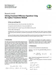
Clearly, (45) are the valid 𝛼-cuts of the solution of (36). For numerical approximation, we set 𝑡 ∈ [0, 2] and 𝑁 = 100. By using Algorithm 1, the results for different values of 𝛽 are plotted in Figure 1. From the graphs, we can see that if 𝛽 approaches 1, the approximate solutions will approach the approximate solution of fuzzy differential equation. Numerical values at 𝑡 = 2 for different values of 𝛽 are listed in Table 1. Example 2. Consider the following linear fuzzy fractional differential equation: 𝑐

𝛽

𝐷0 𝑋 (𝑡) = −𝑋 (𝑡) , 𝑋 (0) = 𝑋0 .

(46)

The nonfuzzy problem associated with (46) is 𝑐

𝛽

𝐷0 𝑥 (𝑡) = −𝑥 (𝑡) , 𝑥 (0) = 𝑥0 .

(47)


7 Table 1: Numerical solutions of Example 1 with different values of 𝛽.

𝛼

𝛽 = 0.6

𝛽

𝑥1 (𝑡) 26063.941926 28670.336119 31276.730311 33883.124504 36489.518697 39095.912889 41702.307082 44308.701274 46915.095467 49521.489660 52127.883852

0.0 0.1 0.2 0.3 0.4 0.5 0.6 0.7 0.8 0.9 1.0

𝛽

𝛽

𝑥2 (𝑡) 78191.825779 75585.431586 72979.037394 70372.643201 67766.249008 65159.854816 62553.460623 59947.066430 57340.672238 54734.278045 52127.883852

𝛽 = 0.8

𝑥1 (𝑡) 98.369851 108.206836 118.043821 127.880806 137.717791 147.554776 157.391761 167.228746 177.065732 186.902717 196.739702

𝛽

𝛽

𝑥2 (𝑡) 295.109553 285.272568 275.435583 265.598598 255.761613 245.924627 236.087642 226.250657 216.413672 206.576687 196.739702

𝛽=1

𝑥1 (𝑡) 7.244646 7.969110 8.693575 9.418039 10.142504 10.866969 11.591433 12.315898 13.040363 13.764827 14.489292

𝛽

𝑥2 (𝑡) 21.733938 21.009473 20.285009 19.560544 18.836079 18.111615 17.387150 16.662686 15.938221 15.213756 14.489292

After simplifying, we get

1 𝛼 0.5

L {𝑥 (𝑡)} =

0 8 ×104

6 X(t)

4

2

0

0.5

0

1.5

1

𝑥0 𝑠𝛽−1 . 𝑠𝛽 + 1

(50)

2

By taking the inverse Laplace transform to (50), we obtain

t

(a)

𝑥 (𝑡) = 𝑥0 L−1 {

1 𝛼 0.5

𝑠𝛽−1 }, 𝑠𝛽 + 1

(51)

which finally has the following solution:

0 300

200 X(t)

100

0

0.5

0

1

1.5

2

𝑥 (𝑡) = 𝑥0 𝐸𝛽 (−𝑡𝛽 ) ,

t

(52)

(b)

where 𝐸𝛽 (∗) is the Mittag-Leffler function. Using Zadeh’s extension principle to (52) in relation to 𝑥0 , we obtain the solution of (46) as follows:

1 𝛼 0.5

0 30

20 X(t)

10

0

0.5

0

1.5

1

𝑋 (𝑡) = 𝑋0 𝐸𝛽 (−𝑡𝛽 ) .

2

t

(c)

Figure 1: The numerical solution of (36) for (a) 𝛽 = 0.6, (b) 𝛽 = 0.8, and (c) 𝛽 = 1.

Let [𝑋(𝑡)]𝛼 = [𝑥1𝛼 (𝑡), 𝑥2𝛼 (𝑡)] and 𝑋0 = (2, 3, 4) where [𝑋0 ]𝛼 = [𝛼 + 2, 4 − 𝛼] for 𝛼 ∈ [0, 1]; then the first ten terms of (52) can be expressed as follows: 𝑥1𝛼 (𝑡) = (𝛼 + 2) (−1 −

In order to find the solution of (46), we first find the solution of (47). By taking the Laplace transform on both sides of (47), we have 𝛽

L { 𝑐 𝐷0 𝑥 (𝑡)} = −L {𝑥 (𝑡)} .

(48)

𝛽−1

𝑠 L {𝑥 (𝑡)} − 𝑥 (𝑡0 ) 𝑠

= −L {𝑥 (𝑡)} .

(49)

𝑡𝛽 𝑡2𝛽 − Γ (𝛽 + 1) Γ (2𝛽 + 1)

−

𝑡3𝛽 𝑡4𝛽 𝑡5𝛽 − − Γ (3𝛽 + 1) Γ (4𝛽 + 1) Γ (5𝛽 + 1)

−

𝑡6𝛽 𝑡7𝛽 − Γ (6𝛽 + 1) Γ (7𝛽 + 1)

−

𝑡8𝛽 𝑡9𝛽 − ), Γ (8𝛽 + 1) Γ (9𝛽 + 1)

It follows that 𝛽

(53)

8

The Scientific World Journal Table 2: Numerical solutions of Example 2 with different values of 𝛽.

𝛼

𝛽 = 0.6

𝛽

𝑥1 (𝑡) 0.000024 0.000025 0.000026 0.000027 0.000029 0.000030 0.000031 0.000032 0.000033 0.000035 0.000036

0.0 0.1 0.2 0.3 0.4 0.5 0.6 0.7 0.8 0.9 1.0

𝛽

𝛽

𝑥2 (𝑡) 0.000048 0.000047 0.000046 0.000044 0.000043 0.000042 0.000041 0.000040 0.000038 0.000037 0.000036

𝑥2𝛼 (𝑡) = (4 − 𝛼) (−1 −

𝛽 = 0.8

𝛽

𝑥1 (𝑡) 0.016304 0.017119 0.017934 0.018750 0.019565 0.020380 0.021195 0.022010 0.022826 0.023641 0.024456

𝑡𝛽 𝑡2𝛽 − Γ (𝛽 + 1) Γ (2𝛽 + 1)

0 4

3 X(t)

2

1

0

1 t

1.5

2

1 t

1.5

2

0.5

0.5

1 t

1.5

2

0.5

0 (a)

9𝛽

𝑡 𝑡 − ). Γ (8𝛽 + 1) Γ (9𝛽 + 1)

1

(54)

𝛼 0.5

Clearly, (54) are the valid 𝛼-cuts of the solution of (46). By using Algorithm 1 with the same interval 𝑡 and interval 𝑁 as in Example 1, the numerical solutions of (46) for different values of 𝛽 are plotted in Figure 2. Again, we can see that the numerical solutions will approach the numerical solution of fuzzy differential equation as 𝛽 increases to 1. Numerical solutions at 𝑡 = 2 for different values of 𝛽 are listed in Table 2.

0 4

0 4

3 X(t)

(55)

1

0

0

𝛼 0.5

𝛽

𝑋 (0) = 𝑋0 ,

2 X(t)

1

Example 3. Let us consider the following problem: 𝐷0 𝑋 (𝑡) = cos (𝑡𝑋) ,

3

(b)

In the following example, we provide detailed procedures for solving a nonlinear fuzzy fractional differential equation.

𝑐

𝛽

𝑥2 (𝑡) 0.530478 0.517216 0.503954 0.490692 0.477430 0.464168 0.450906 0.437644 0.424382 0.411120 0.397858

𝛼 0.5

𝑡6𝛽 𝑡7𝛽 − − Γ (6𝛽 + 1) Γ (7𝛽 + 1) −

𝑥1 (𝑡) 0.265239 0.278501 0.291763 0.305024 0.318286 0.331548 0.344810 0.358072 0.371334 0.384596 0.397858

1

𝑡3𝛽 𝑡4𝛽 𝑡5𝛽 − − − Γ (3𝛽 + 1) Γ (4𝛽 + 1) Γ (5𝛽 + 1)

8𝛽

𝛽=1

𝛽

𝑥2 (𝑡) 0.032608 0.031793 0.030978 0.030163 0.029347 0.028532 0.027717 0.026902 0.026087 0.025271 0.024456

2

1

0

0 (c)

Figure 2: The numerical solutions of (46) for (a) 𝛽 = 0.6, (b) 𝛽 = 0.8, and (c) 𝛽 = 1.

where 𝛽 ∈ (0, 1], 𝑡 = [0, 5], and 𝑋0 is any triangular fuzzy number. To solve this problem, we use Algorithm 2. First, let 𝛼 𝛼 , 𝑥0,2 ]. We discretise 𝛼 up to 11 points, which [𝑋0 ]𝛼 = [𝑥0,1 are 𝛼0 = 0 < 𝛼1 = 0.1 < ⋅ ⋅ ⋅ < 𝛼10 = 1. Let 𝑋0 = 𝑊0 ; then we have 𝛼 𝑤1,110

𝛼 𝑔 (𝛽, ℎ, 𝑡0 , 𝑤0,110 )

=

=

𝛼 𝑔 (𝛽, ℎ, 𝑡0 , 𝑤0,210 )

=

𝛼 𝑤1,210 ,

𝛼 𝛼 𝑤2,29 = max [ max 𝑔 (𝛽, ℎ, 𝑡1 , 𝑢) , 𝑤1,210 , max 𝑔 (𝛽, ℎ, 𝑡1 , 𝑢)] , 𝛼9 𝛼10 𝛼10 𝛼9 𝑢∈[𝑤1,1 ,𝑤1,1 ] 𝑢∈[𝑤1,2 ,𝑤1,2 ] [ ]

.. . 𝛼

𝛼 min 𝑔 (𝛽, ℎ, 𝑡1 , 𝑢) , 𝑤1,110 , min 𝑔 (𝛽, ℎ, 𝑡1 , 𝑢)] , 𝛼9 𝛼10 𝛼10 𝛼9 𝑢∈[𝑤1,1 ,𝑤1,1 ] 𝑢∈[𝑤1,2 ,𝑤1,2 ]

= min [ [

1 min 𝑔 (𝛽, ℎ, 𝑡𝑁 , 𝑢) , 𝑤𝑁,1 , 𝛼 𝛼

0 1 ] 𝑢∈[𝑤𝑁,1 ,𝑤𝑁,1

𝛼

𝛼 𝑤2,19

𝛼

0 𝑤𝑁+1,1 = min [

]

0 = max [ 𝑤𝑁+1,2

𝛼

1 max 𝑔 (𝛽, ℎ, 𝑡𝑁 , 𝑢) , 𝑤𝑁,2 , 𝛼 𝛼

0 1 ] 𝑢∈[𝑤𝑁,1 ,𝑤𝑁,1

min 𝑔 (𝛽, ℎ, 𝑡𝑁 , 𝑢)] , 𝛼 𝛼

1 ,𝑤 0 ] 𝑢∈[𝑤𝑁,2 𝑁,2

max 𝑔 (𝛽, ℎ, 𝑡𝑁 , 𝑢)] , 𝛼 𝛼

1 ,𝑤 0 ] 𝑢∈[𝑤𝑁,2 𝑁,2

(56)


9 Table 3: Numerical solutions of Example 3 with different values of 𝛽.

𝛼

𝛽 = 0.6

𝛽

𝑥1 (𝑡) 0.316778 0.316778 0.316778 0.316778 0.316778 0.316778 0.316778 0.316778 0.316778 0.316778 0.316778

0.0 0.1 0.2 0.3 0.4 0.5 0.6 0.7 0.8 0.9 1.0

𝛽

𝛽

𝑥2 (𝑡) 0.316778 0.316778 0.316778 0.316778 0.316778 0.316778 0.316778 0.316778 0.316778 0.316778 0.316778

𝑥1 (𝑡) 0.320052 0.320052 0.320052 0.320052 0.320052 0.320052 0.320052 0.320052 0.320052 0.320052 0.320052

𝛼 0.5

4 X(t)

2

0

0

1

2

3

t

5

4

𝛽=1

𝛽

𝑥2 (𝑡) 1.645658 1.645476 1.643608 0.328664 0.328629 0.328617 0.328610 0.328606 0.328604 0.328602 0.328600

In this paper, we have studied a fuzzy fractional differential equation and presented its solution using Zadeh’s extension principle. The classical fractional Euler method has also been extended in the fuzzy setting in order to approximate the solutions of linear and nonlinear fuzzy fractional differential equations. Final results showed that the solution of fuzzy fractional differential equations approaches the solution of fuzzy differential equations as the fractional order approaches the integer order.

1 𝛼 0.5 3 X(t)

2

1

0

0

1

2

3 t

5

4

(b)

Acknowledgments

1

This research was supported by the Short Term Grant (STG) of Universiti Malaysia Perlis (UniMAP) under the Project code 9001-00319 and partially supported by Research Acculturation Grant Scheme (RAGS) under the Project code 901800003.

𝛼 0.5 0 4

𝛽

𝑥1 (𝑡) 0.328592 0.328592 0.328593 0.328594 0.328594 0.328595 0.328596 0.328597 0.328598 0.328599 0.328600

5. Conclusions

(a)

0 4

𝛽

𝑥2 (𝑡) 0.320052 0.320052 0.320052 0.320052 0.320052 0.320052 0.320052 0.320052 0.320052 0.320052 0.320052

see that the numerical solutions approach to the numerical solution of fuzzy differential equation as 𝛽 approaches 1. Numerical solutions at 𝑡 = 5 at different values of 𝛽 are listed in Table 3.

1

0 6

𝛽 = 0.8

3 X(t)

2

1

0

0

1

2

t

3

5

4

References

(c)

Figure 3: The approximate solutions of (55) for (a) 𝛽 = 0.6, (b) 𝛽 = 0.8, and (c) 𝛽 = 1.

where 𝑔 (𝛽, ℎ, 𝑡𝑖 , 𝑢) = 𝑢 +

ℎ𝛽 cos (𝑡𝑖 𝑢) , Γ (𝛽 + 1)

𝛼

𝛼

𝑢 ∈ [𝑤𝑖,1𝑗 , 𝑤𝑖,2𝑗 ] (57)

for 𝑖 = 0, 1, . . . , 𝑁 and 𝑗 = 0, 1, . . . , 10. Let 𝑋0 = (0, 𝜋/2, 𝜋) and 𝑁 = 200; then these procedures will result in the approximate solutions of (55) at different values of 𝛽 as plotted in Figure 3. From the graphs, we can

[1] G. Jumarie, “Table of some basic fractional calculus formulae derived from a modified Riemann-Liouville derivative for nondifferentiable functions,” Applied Mathematics Letters, vol. 22, no. 3, pp. 378–385, 2009. [2] J. J. Trujillo, M. Rivero, and B. Bonilla, “On a Riemann-Liouville generalized Taylor’s formula,” Journal of Mathematical Analysis and Applications, vol. 231, no. 1, pp. 255–265, 1999. [3] G. A. Anastassiou, “Opial type inequalities involving RiemannLiouville fractional derivatives of two functions with applications,” Mathematical and Computer Modelling, vol. 48, no. 3-4, pp. 344–374, 2008. [4] Y. S. Liang, “Box dimensions of Riemann-Liouville fractional integrals of continuous functions of bounded variation,” Nonlinear Analysis: Theory, Methods & Applications, vol. 72, no. 11, pp. 4304–4306, 2010.

10 [5] I. Podlubny, “Riesz potential and Riemann-Liouville fractional integrals and derivatives of Jacobi polynomials,” Applied Mathematics Letters, vol. 10, no. 1, pp. 103–108, 1997. [6] R. Almeida and D. F. M. Torres, “Calculus of variations with fractional derivatives and fractional integrals,” Applied Mathematics Letters, vol. 22, no. 12, pp. 1816–1820, 2009. [7] Z. Wei, W. Dong, and J. Che, “Periodic boundary value problems for fractional differential equations involving a RiemannLiouville fractional derivative,” Nonlinear Analysis: Theory, Methods & Applications, vol. 73, no. 10, pp. 3232–3238, 2010. [8] Z. Wei, Q. Li, and J. Che, “Initial value problems for fractional differential equations involving Riemann-Liouville sequential fractional derivative,” Journal of Mathematical Analysis and Applications, vol. 367, no. 1, pp. 260–272, 2010. [9] D. Qian, C. Li, R. P. Agarwal, and P. J. Y. Wong, “Stability analysis of fractional differential system with Riemann-Liouville derivative,” Mathematical and Computer Modelling, vol. 52, no. 5-6, pp. 862–874, 2010. [10] S. G. Samko, A. A. Kilbas, and O. I. Marichev, Fractional Integrals and Derivatives: Theory and Applications, Gordon and Breach, Yverdon, Switzerland, 1993. [11] I. Podlubny, Fractional Differential Equation, Academic Press, 1999. [12] V. Daftardar-Gejji and H. Jafari, “Analysis of a system of nonautonomous fractional differential equations involving Caputo derivatives,” Journal of Mathematical Analysis and Applications, vol. 328, no. 2, pp. 1026–1033, 2007. [13] D. A. Murio, “On the stable numerical evaluation of Caputo fractional derivatives,” Computers and Mathematics with Applications, vol. 51, no. 9-10, pp. 1539–1550, 2006. [14] Z. M. Odibat, “Computing eigenelements of boundary value problems with fractional derivatives,” Applied Mathematics and Computation, vol. 215, no. 8, pp. 3017–3028, 2009. [15] V. S. Ertürk and S. Momani, “Solving systems of fractional differential equations using differential transform method,” Journal of Computational and Applied Mathematics, vol. 215, no. 1, pp. 142–151, 2008. [16] V. S. Ertürk, S. Momani, and Z. Odibat, “Application of generalized differential transform method to multi-order fractional differential equations,” Communications in Nonlinear Science and Numerical Simulation, vol. 13, no. 8, pp. 1642–1654, 2008. [17] K. S. Miller and B. Ross, An Introduction to the Fractional Calculus and Differential Equations, John Wiley & Sons, New York, NY, USA, 1993. [18] K. Diethelm and N. J. Ford, “Analysis of fractional differential equations,” Journal of Mathematical Analysis and Applications, vol. 265, no. 2, pp. 229–248, 2002. [19] V. Lakshmikantham and R. N. Mohapatra, Theory of Fuzzy Differential Equations and Applications, Taylor & Francis, London, UK, 2003. [20] A. A. Kilbas, H. M. Srivastava, and J. J. Trujillo, Theory and Applications of Fractional Differential Equations, Elsevier Science B.V, Amsterdam, The Netherlands, 2006. [21] V. Lakshmikantham and A. S. Vatsala, “Basic theory of fractional differential equations,” Nonlinear Analysis: Theory, Methods & Applications, vol. 69, no. 8, pp. 2677–2682, 2008. [22] V. Lakshmikantham and S. Leela, “Nagumo-type uniqueness result for fractional differential equations,” Nonlinear Analysis: Theory, Methods & Applications, vol. 71, no. 7-8, pp. 2886–2889, 2009.

The Scientific World Journal [23] S. Zhang, “Monotone iterative method for initial value problem involving Riemann-Liouville fractional derivatives,” Nonlinear Analysis: Theory, Methods & Applications, vol. 71, no. 5-6, pp. 2087–2093, 2009. [24] H. Jafari, H. Tajadodi, and S. A. Hosseini Matikolai, “Homotopy perturbation pade technique for solving fractional Riccati differential equations,” The International Journal of Nonlinear Sciences and Numerical Simulation, vol. 11, pp. 271–276, 2011. [25] H. Jafari, H. Tajadodi, H. Nazari, and C. M. Khalique, “Numerical solution of non-linear Riccati differential equations with fractional order,” The International Journal of Nonlinear Sciences and Numerical Simulation, vol. 11, pp. 179–182, 2011. [26] F. B. Adda and J. Cresson, “Fractional differential equations and the Schrödinger equation,” Applied Mathematics and Computation, vol. 161, no. 1, pp. 323–345, 2005. [27] Z. E. A. Fellah, C. Depollier, and M. Fellah, “Application of fractional calculus to the sound waves propagation in rigid porous materials: validation via ultrasonic measurements,” Acta Acustica united with Acustica, vol. 88, no. 1, pp. 34–39, 2002. [28] M. Rahimy, “Applications of fractional differential equations,” Applied Mathematical Sciences, vol. 4, no. 49–52, pp. 2453–2461, 2010. [29] M. Z. Ahmad and B. De Baets, “A predator-prey model with fuzzy initial populations,” in Proceedings of the 13th IFSA World Congress and 6th European Society of Fuzzy Logic and Technology Conference, pp. 1311–1314, 2009. [30] L. A. Zadeh, “Fuzzy sets,” Information and Control, vol. 8, no. 3, pp. 338–353, 1965. [31] R. P. Agarwal, V. Lakshmikantham, and J. J. Nieto, “On the concept of solution for fractional differential equations with uncertainty,” Nonlinear Analysis: Theory, Methods & Applications, vol. 72, no. 6, pp. 2859–2862, 2010. [32] S. Arshad and V. Lupulescu, “On the fractional differential equations with uncertainty,” Nonlinear Analysis: Theory, Methods & Applications, vol. 74, no. 11, pp. 3685–3693, 2011. [33] T. Allahviranloo, S. Salahshour, and S. Abbasbandy, “Explicit solutions of fractional differential equations with uncertainty,” Soft Computing, vol. 16, no. 2, pp. 297–302, 2012. [34] S. Salahshour, T. Allahviranloo, and S. Abbasbandy, “Solving fuzzy fractional differential equations by fuzzy Laplace transforms,” Communications in Nonlinear Science and Numerical Simulation, vol. 17, no. 3, pp. 1372–1381, 2012. [35] T. Allahviranloo and M. B. Ahmadi, “Fuzzy Laplace transforms,” Soft Computing, vol. 14, no. 3, pp. 235–243, 2010. [36] O. Kaleva, “Fuzzy differential equations,” Fuzzy Sets and Systems, vol. 24, no. 3, pp. 301–317, 1987. [37] S. Seikkala, “On the fuzzy initial value problem,” Fuzzy Sets and Systems, vol. 24, no. 3, pp. 319–330, 1987. [38] O. Kaleva, “A note on fuzzy differential equations,” Nonlinear Analysis: Theory, Methods & Applications, vol. 64, no. 5, pp. 895– 900, 2006. [39] B. Bede, I. J. Rudas, and A. L. Bencsik, “First order linear fuzzy differential equations under generalized differentiability,” Information Sciences, vol. 177, no. 7, pp. 1648–1662, 2007. [40] B. Bede and S. G. Gal, “Generalizations of the differentiability of fuzzy-number-valued functions with applications to fuzzy differential equations,” Fuzzy Sets and Systems, vol. 151, no. 3, pp. 581–599, 2005. [41] M. Z. Ahmad and M. K. Hasan, “Numerical methods for fuzzy initial value problems under different types of interpretation: a comparison study,” in Informatics Engineering and Information


[42] [43]

[44]

[45]

[46]

[47]

[48]

[49]

[50]

[51]

[52] [53]

[54]

[55]

[56] [57]

[58]

[59]

Science, vol. 252 of Communications in Computer and Information Science, pp. 275–288, Springer, Berlin, Germany, 2011. J. J. Buckley and T. Feuring, “Fuzzy differential equations,” Fuzzy Sets and Systems, vol. 110, no. 1, pp. 43–54, 2000. M. T. Mizukoshi, L. C. Barros, Y. Chalco-Cano, H. RománFlores, and R. C. Bassanezi, “Fuzzy differential equations and the extension principle,” Information Sciences, vol. 177, no. 17, pp. 3627–3635, 2007. Y. Chalco-Cano and H. Román-Flores, “On new solutions of fuzzy differential equations,” Chaos, Solitons & Fractals, vol. 38, no. 1, pp. 112–119, 2008. S. C. Palligkinis, G. Papageorgiou, and I. T. Famelis, “RungeKutta methods for fuzzy differential equations,” Applied Mathematics and Computation, vol. 209, no. 1, pp. 97–105, 2009. Y. Chalco-Cano and H. Román-Flores, “Comparation between some approaches to solve fuzzy differential equations,” Fuzzy Sets and Systems, vol. 160, no. 11, pp. 1517–1527, 2009. M. Z. Ahmad and M. K. Hasan, “A new approach to incorporate uncertainty into Euler’s method,” Applied Mathematical Sciences, vol. 4, no. 49–52, pp. 2509–2520, 2010. M. Z. Ahmad and M. K. Hasan, “A new fuzzy version of Euler’s method for solving differential equations with fuzzy initial values,” Sains Malaysiana, vol. 40, no. 6, pp. 651–657, 2011. M. Z. Ahmad, M. K. Hasan, and B. De Baets, “Analytical and numerical solutions of fuzzy differential equations,” Information Sciences, vol. 236, pp. 156–167, 2013. R. Gorenflo and F. Mainardi, “Fractional calculus: integral and differential equations of fractional order,” in Fractals and Fractional Calculus in Continuum Mechanics, pp. 223–276, Springer, New York, NY, USA, 1997. Y. Li, Y. Chen, and I. Podlubny, “Mittag-Leffler stability of fractional order nonlinear dynamic systems,” Automatica, vol. 45, no. 8, pp. 1965–1969, 2009. L. X. Wang, A Course in Fuzzy Systems and Control, PrenticeHall, Englewood Cliffs, NJ, USA, 1997. M. Z. Ahmad, M. K. Hasan, and B. De Baets, “A new method for computing continuous functions with fuzzy variable,” Journal of Applied Sciences, vol. 11, no. 7, pp. 1143–1149, 2011. M. Z. Ahmad and M. K. Hasan, “Incorporating optimisation technique into Zadeh’s extension principle for computing nonmonotone functions with fuzzy variable,” Sains Malaysiana, vol. 40, no. 6, pp. 643–650, 2011. H. Román-Flores, L. C. Barros, and R. C. Bassanezi, “A note on Zadeh’s extensions,” Fuzzy Sets and Systems, vol. 117, no. 3, pp. 327–331, 2001. R. Goetschel Jr. and W. Voxman, “Elementary fuzzy calculus,” Fuzzy Sets and Systems, vol. 18, no. 1, pp. 31–43, 1986. M. L. Puri and D. A. Ralescu, “Fuzzy random variables,” Journal of Mathematical Analysis and Applications, vol. 114, no. 2, pp. 409–422, 1986. R. P. Agarwal, D. O’Regan, and V. Lakshmikantham, “Viability theory and fuzzy differential equations,” Fuzzy Sets and Systems, vol. 151, no. 3, pp. 563–580, 2005. Z. M. Odibat and S. Momani, “An algorithm for the numerical solution of differential equations of fractional order,” Journal of Applied Mathematics & Informatics, vol. 26, pp. 15–27, 2008.

11

Advances in

Decision Sciences

Advances in

Mathematical Physics Hindawi Publishing Corporation http://www.hindawi.com

Volume 2013

The Scientific World Journal Hindawi Publishing Corporation http://www.hindawi.com

Volume 2013

International Journal of

Mathematical Problems in Engineering Hindawi Publishing Corporation http://www.hindawi.com

Volume 2013

Combinatorics Hindawi Publishing Corporation http://www.hindawi.com

Volume 2013

Volume 2013

Abstract and Applied Analysis

Journal of Applied Mathematics

Hindawi Publishing Corporation http://www.hindawi.com



Volume 2013

Volume 2013

Discrete Dynamics in Nature and Society

Submit your manuscripts at http://www.hindawi.com Journal of Function Spaces and Applications Hindawi Publishing Corporation http://www.hindawi.com


Volume 2013

International Journal of Mathematics and Mathematical Sciences

Advances in

Volume 2013

Journal of

Operations Research

Probability and Statistics International Journal of

Differential Equations Hindawi Publishing Corporation http://www.hindawi.com

Volume 2013

ISRN Mathematical Analysis Hindawi Publishing Corporation http://www.hindawi.com


Volume 2013

ISRN Discrete Mathematics Volume 2013



International Journal of

Stochastic Analysis Volume 2013


Volume 2013

ISRN Applied Mathematics

ISRN Algebra Volume 2013


Volume 2013



Volume 2013

ISRN Geometry Volume 2013


Volume 2013