sustainability Article
Research on Factors Affecting the Optimal Exploitation of Natural Gas Resources in China Jianzhong Xiao 1,2 , Xiaolin Wang 1, * and Ran Wang 2 1 2
*
School of Economics and Management, China University of Geosciences, Wuhan 430074, China;
[email protected] Resources and Environment Economic Research Center, China University of Geosciences, Wuhan 430074, China;
[email protected] Correspondence:
[email protected]; Tel.:+86-27-6788-3201
Academic Editor: Bing Wang Received: 16 January 2016; Accepted: 26 April 2016; Published: 2 May 2016
Abstract: This paper develops an optimizing model for the long-term exploitation of limited natural gas reserves in China. In addition to describing the life cycle characteristics of natural gas production and introducing the inter-temporal allocation theory, this paper builds the optimal exploitation model of natural gas resources within a gas field in the Ordos Basin as an example to analyze its exploitation scale and how influence factors, such as recovery rate, discount rate and the gas well exhausting cycle, affect the optimal exploration path of this gas field. We determine that an increase in the discount rate stimulates investors to invest more aggressively in natural gas exploitation in the early period due to the lower discounted value, thereby increasing the pace of the exploitation of natural gas and the exhaustion of gas fields. A higher recoverable factor implies more recoverable reserves and greater potential of increasing the output of gas fields. The exhaustion rate of gas wells affects the capability of converting capacity to output. When exhaustion occurs quickly in gas wells, the output will likely increase in the output rising period, and the output will likely decrease at a faster rate in the output reduction period. Price reform affects the economic recoverable reserves of gas fields. Keywords: natural gas resources; optimal exploitation model; recovery rate; discount rate; exhausting rate; gas pricing
1. Introduction In this study, we develop an optimizing model for the long-term exploitation of limited natural gas reserves in China, which is a coal-dominated energy structure economy and suffers from serious pollution problems. Nevertheless, natural gas is currently promoted by Chinese authorities due to its relatively low carbon dioxide emissions. Therefore, the Chinese government confirmed its strong determination to increase domestic supply and to narrow the increasing gap between demand and production [1,2]. A large proportion of natural gas supply activities that include exploration, extraction and transportation of gas in China are currently overseen by the National Oil Company (NOC). In the current liberalized environment, investment from the private sector is encouraged. Upstream activities (exploration and extraction) are in dire need of investment, and because these investments are scarce resources, they need to be spread among various potentially productive basins. According to Dai et al. [3], conventional gas geological resources in China have increased from (5.4–7) ˆ1012 m3 in 1981 to 63 ˆ 1012 m3 in 2010; these data have been assessed by various scholars and divisions over the past thirty years and, thus, are validated. China recorded (39.0–39.2) ˆ 1012 m3 recoverable conventional gas resources; this is an immense amount for any type of major gas producer and will provide a solid foundation for the sustainable development of China’s natural gas industry. Sustainability 2016, 8, 435; doi:10.3390/su8050435
www.mdpi.com/journal/sustainability
Sustainability 2016, 8, 435
2 of 13
However, large gas fields in China are mainly distributed in the mid-west and include the Ordos Basin, the Sichuan Basin and the Tarim Basin. The “gold” buried at the depths of reserves is deeper than that abroad with low pressure and a low discovery rate, i.e., the reserves buried at depths of 3000–4500 m account for 46.11% of the total reserves of China. Hence, their exploration will be more difficult, generate higher costs and have a greater environmental influence. As a result, the well-head price of gas in China is equivalent to the border prices of Europe’s imported gas from Russia. The influence of factors, such as geology, technology, policy and regulation, makes it difficult to effectively convert China’s gas reserves into economic output, thereby preventing natural gas enterprises from generating more profits. The effective exploitation of existing natural gas under varying conditions has become a primary concern for major oil-gas enterprises. Thus, it is vital to analyze corresponding incentives, including economic, technological and regulation factors, which shape the optimizing paths in China. Given the lack of peer-reviewed studies regarding the Chinese natural gas industry, this study aims to fill this gap by developing an optimizing approach to model gas production in China. Furthermore, this study contributes to investment planning and policy-making processes related to the gas production in China. This paper is organized as follows: A literature review is provided in Section 2. Section 3 presents the model’s structure and its general description. Section 4 explains the optimal exploitation path of natural gas resources, Section 5 describes the primary results of the simulation analysis, and Section 6 provides the conclusion. 2. Literature Review The issues of optimal nonrenewable resource extraction were first proposed by Hotelling [4], whose basic model predicted that the shadow price of resource stock, which is a classic measure of the scarcity of the resource, should increase at the rate of interest. Since the time of Hotelling’s study, economists have expanded on his theoretical framework to allow for more realistic features. The impact of exploration activities and an extension of the resource reserves on the Hotelling framework were first suggested by Meadows et al. [5], and Solow’s publication on Hotelling’s model [6] boosted interest in the theory of nonrenewable resource extraction. These scholars demonstrate that exploration activities and the resource price and production path are related [7]; an increase in reserves is generally followed by an increase in production [8,9]. However, as the discovery of further reserves increases to the threshold and exploration activity declines, production also decreases. Additional analyses have been conducted, which Chermak and Patrick [10,11] classified into two primary groups: price path tests and price behavior tests. Price path tests examine if the price of a nonrenewable resource changes according to Hotelling’s “r-percent rule” (i.e., whether the price increases at the rate of interest). None of the price path analyses conducted by Barnett and Morse [12], could produce evidence for the theory using actual data [13,14]. However, these tests include strong assumptions that result from simplifications in Hotelling’s model. First, technology is assumed to be constant over time, and second, the relation of extraction and production costs to the resource base is not considered. Large-scale optimization models have been successfully implemented in the copper sector [15,16], as well as in other natural resource industries (e.g., Epstein et al. in the forest industry [17] or Baker and Ladson [18], and Dyer et al. [19], in the crude oil industry). Based on these systems, decision-makers are able to evaluate alternative operational policies and select those that maximize short-term and long-term profits of the business. However, for most of these models, deterministic inputs in the methodology include the net discounted value, which is predominately used by businesses. The model utilized in this study builds on Ellis and Halvorsen [20] and Pindyck [21] regarding exploration activity. However, our model has substantially broadened the representation of the gas industry beyond that found in Pindyck’s model. In particular, we attempt to address limitations that, in our opinion, made Pindyck’s model a less realistic representation for the specific case of indigenous Chinese gas production. For this reason, beginning with the economic theory of optimal resources exploitation, this paper constructs the exploitation model of resources in combination with the theories of optimal control, net
Sustainability 2016, 8, 435
3 of 13
present value and dynamic life cycle. In addition, this study developed a broadened model for the assessment of the effect of technical, cost and policy factors on the optimal exploitation of natural gas resources in China. The contribution of this study is in building the model under dynamic reserves by combining gas field benefits, gas well life cycles and gas field recovery rates into the optimal path model. The results and conclusions will be helpful for the government to formulate policies and for enterprises to make decisions. 3. Optimal Exploitation Model of Natural Gas Resources 3.1. Objective Function The net present value of total revenue generated from natural gas within the life cycle of natural gas exploitation is presented as follows: V“
Tÿ ´1
e´rt rPt Xt ´ Ct s
(1)
t “0
where Pt represents the market price of oil and gas resources of year t, Xt represents the exploitation volume of natural gas of year t, e´ rt represents the discount coefficient and Ct represents the total cost of natural gas exploitation of year t, including exploration cost, exploitation cost and production cost. The objective of natural gas exploitation is to maximize the value of exploitation, namely: maxV “
Tÿ ´1
e
´rt
rPt Xt ´ Ct s
(2)
t“0
3.2. Constraint Conditions Because natural gas is non-renewable, reserves will decrease with constant exploitation, thus satisfying: $ r t`τ ’ Kt piqdi & pQt`1 ´ Qt q ˆ h “ ´ t Q0 “ Sp0q ’ % Q “ SpTq T
pt “ 0, 1, 2, ¨ ¨ ¨ ¨ ¨ ¨ , T ´ 1; i “ 0, 1, ¨ ¨ ¨ , τ ´ 1q
(3)
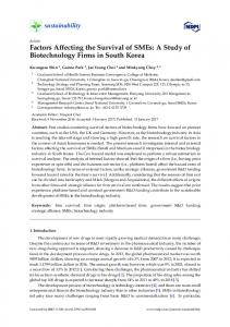
where T represents the total number of years that gas resources can be exploited; Qt represents the remaining reserves and state variable of natural gas at the beginning of year t; h represents the recovery rate in the gas field; τ represents the life cycle of gas wells; i denotes the parameter of the period(year) between t and t ` τ; Kt piq represents gas production volume of the t batch of gas wells within the r t`τ life cycle of τ years; and t Kt piqdi represents the total exploitation volume of the t batch of gas r t`τ wells within the life cycle of τ years. pQt`1 ´ Qt q ˆ h “ ´ t Kt piqdi is a set of differential equations, modifying the transfer law from state t to state t ` 1. Sp0q denotes the initial reserves and SpTq the reserves at time T at the end of the period. In general, exploitation volume Xt is realized through the production volume of different batches of gas wells at time t. Every batch of gas wells experiences an output rising period, a stable period and an output reduction period within a life cycle of τ years; however, the output functions of each batch of gas wells within the life cycle are not necessarily consistent (Figure 1). Let Kt piq denote the exploitation function of the t batch of gas wells in period i within the life cycle of τ years. The following four inverted “U-shaped” curves demonstrate the schematic diagrams of converting the capacity of different batches of gas wells to output. The production curve is inverted and declines sharply because each well has a short life cycle. Hence, the incremental curve is the accumulative production for the gas fields. In consideration of the functionality of the graph, the schematic diagrams of gas well exhaustion for other years are not plotted.
Sustainability 2016, 8, x
4 of 13
inverted and declines sharply because each well has a short life cycle. Hence, the incremental curve is the accumulative Sustainability 2016, 8, 435 production for the gas fields. In consideration of the functionality of the graph, 4 of 13 the schematic diagrams of gas well exhaustion for other years are not plotted.
t1 t2
t1 t2 t3
……
t3
…
Figure 1. Velocity of converting the capacity of different batches of gas wells to output. Figure 1. Velocity of converting the capacity of different batches of gas wells to output. t
r t`τK (i)d of the t batch of gas wells Assuming the t piqd i K Assuming the life life cycle cycleof ofgas gaswells wellsisisτ,, the the capacity capacity tt t i of the t batch of gas wells utilized in be converted to output between yearyear t and tyear τ. For fields, natural in year yeart will be converted to output between andt ` year . For gasthe fields, the t +gas t will gas exploitation volume of year t of is the total the total natural gas natural produced the t ` τ by batch natural gas exploitation volume yearsum theofsum of the gasby produced the and t +t t is batch gast wells at of time The conversion theconversion capacity ofofdifferent batches gas wells satisfies the batch of and batch gast.wells at time t . of The the capacity of of different batches of gas following equation: wells satisfies the following equation: #
1 2 r1 r ri i t 1 r Kt 1 (xx)`d x¨ ¨¨… )d x x… Xptq “ 0X(t)= Kt pxqd ` i´i 11 Ktt´i i1`( 1xpxqd `+¨¨t ¨`Kttt´τ`1 1 (τx) dK i t´1 pxqdi 0 Kx t`( x)1d2 xKt´11 pxqd ´ ri i xK“ ( xf)pt, d x iq f (t , i ) i´1 Kt pxqd i 1 t
(4) (4)
where P [0, r0,TTs. [0,τs, ], tt ]. where i iPr0, We denote K piq the of gas wells at at time i within the life i within We denote Kt t (i)asas theexploitation exploitationfunction functionofofthe thet batch of gas wells time the t batch cycle of τ years; r i of years; life cycle i 1 Kt pxqd x denotes the exploitation volume of the t batch of gas wells at time i within the life i´ denotes the exploitation volume of the t batch of gas wells at time i within the t ( x) d x cycle of τKyears. i 1
life cycle of years. 3.3. Optimal Conditions 3.3. Optimal Conditions The above objective function and constraint conditions constitute the inter-temporal optimized model of natural gas optimal exploitation, namely the optimal exploitation model ofoptimized dynamic The above objective function and constraint conditions constitute the inter-temporal natural gasnatural resources. modelexploitation, of the reasonable natural gas exploitation scale model is transformed into model of gasThe optimal namely the optimal exploitation of dynamic an unconstrained Lagrange extremum problem with T ´ 1 constraint conditions, as demonstrated below natural gas resources. The model of the reasonable natural gas exploitation scale is transformed into: an unconstrained problem r with T 1 constraint conditions, Tř ´1 Lagrange extremum Tř ´1 t`τ L “below: e´rt rPt Xt ´ Cs ` te´rpt`1q λt`1 r´ t Kt pxqd x ` pQt`1 ´ Qt q ˆ hsu demonstrated
“
t “0 Tř ´1 t “0
T 1
t “0
T 1
t τ ( r t +1ř ) Le´rt et X[t P´ C ]e´ r iq `KpQ d1x ´ (Q Qtt q1ˆ hsu Qt) h]} trP λt{`e1 r´ t f1[pt, t XCs t ` t ( xt)` t rt
t 0
t 0
as
(5)
i “1
(5) e {[ P X C ] e [ f ( t , i ) ( Q Q ) h]} t t t 1 t 1 t To calculate the extremum conditions for Equation (5), the Hamilton function is introduced; let: T 1
rt
r
t 0
i 1
$ rλ HpXt , Q, λfor tq “ Pt Xt (5), ´ e´the To calculate the extremum Hamilton function is introduced; & H “conditions t`1 ,Equation t` 1 Fptq τ ř (6) let: f pt, iq % Fptq “ i “1
Sustainability 2016, 8, 435
5 of 13
Substituting Equation (5) into Equation (6) produces the following: L“
Tÿ ´1
rH`e´r λt`1 pQt`1 ´ Qt q ˆ hse´rt
(7)
t“0
Conditions necessary to take the extreme value in Equation (7): $ BH ´r ’ ’ B Xt “ Pt ´ MC ´ e λt`1 “ 0 ’ ’ & BH ´ r p t `1 q λ ´rt λ “ 0 t t `1 ´ e B Qt “ e ’ τ ř ’ BH ’ ’ f pt, iq ` pQt`1 ´ Qt q ˆ h “ 0 % B λt`1 “ ´
pt “ 0, 1, 2, ¨ ¨ ¨ ¨ ¨ ¨ , T ´ 1q
(8)
i“1
MC represents the marginal cost. The optimal conditions for Equation (5) can be derived from Equations (6)–(8): $ ’ Pt ´ MC ´ e´r λt`1 “ 0 & pt “ 0, 1, 2, ¨ ¨ ¨ ¨ ¨ ¨ , T ´ 1q (9) e ´ r λ t `1 “ λ t ’ % pQ t`1 ´ Qt q ˆ h “ ´Fptq Substitute Equations (8) and (9) into Equation (7); we calculate the following: Pt ´ MC ´ ert λ0 “ 0 pt “ 0, 1, 2, ¨ ¨ ¨ ¨ ¨ ¨ , T ´ 1q
(10)
It can be determined from the above equation sets that λ0 ˚ and optimal path Xt ˚ can be obtained as long as the functional relations between MC, Qt , Xt , h and Kt piq in different time periods are available. 4. Optimal Exploitation Path of Natural Gas Resources 4.1. Parameters Setting Based on the above model analysis, this section selects a gas field in the Ordos Basin as the research target and simulates scenarios to solve for the optimal exploitation scale. The selected gas field is typical, features “three lows” (low porosity, low permeability and low pressure) and represents an onshore gas field in China. This gas field has been exploited for more than ten years and is currently in the output rising period. The analysis of the parameters involved in this study is described in the following text. 4.1.1. Gas Field Exhausting Time T Because the optimal exhausting rate (an analytical solution with implicit T) involves the setting of time T, the optimal exploitation scale can be solved according to the inter-temporal optimized model of natural gas exploitation scale when T is set. In addition, a gas field has a life cycle. The gas field in the Ordos Basin has a short production period, so its life cycle is divided into three periods (i.e., output rising period, stable period and output reduction period) with tk , ts ´ tk and T ´ ts denoting the corresponding years for each period. In this section, the life cycle of this gas field is denoted as T “ 40 years, of which tk “ 12 years are in the output rising period, ts ´ tk “ 13 years are in the stable period and T ´ ts “ 15 years are in the output reduction period. 4.1.2. Marginal Exploitation Cost of Natural Gas MC We consider the fact that estimation of the marginal cost represents the optimization problem of the gas producer. From a modeling perspective, we would prefer the marginal cost to depend on the actual sequence of extraction. This consideration in our formulation is particularly useful for modeling underground mining operations in which production costs tend to increase as extraction progresses. This assumption allows us to formulate the decision-maker’s optimization problem
Sustainability 2016, 8, 435
6 of 13
using linear programming methods. The exploitation cost of natural gas C refers to the total costs incurred during the development of natural gas, particularly the exploration cost, development cost and production cost. For simplicity, this study assumes that the marginal costs of exploration and development are constant. In regards to the cost of production, this study divides the exhausting period T of the gas field into the output rising period, the stable period and the output reduction period according to its life cycle. Combining the above hypotheses, the marginal cost of production within period T is determined as demonstrated below: $ ’ & MCPptq “ at ` b p1 ď t ď tk q (11) MCPptq “ c ptk ď t ď ts q ’ % MCPptq “ dt ` e pt ď t ď Tq s where MCPptq represents the marginal cost of production at time t and a, b, c, d, e are the coefficients of the marginal cost of production MCPptq in different time periods. Marginal costs are determined according to the life cycle. The marginal cost of exploration is MCE “ 0.05 CNY/m3 ; the marginal cost of development is MCD “ 0.05 CNY/m3 ; and the coefficients of the marginal cost of production MCPptq are a “ 0.02, b “ 0.082, c “ 0.056, d “ 0.004, e “ ´0.04. 4.1.3. Discount Rate r In addition to a risk-free discount rate, the discount rate should consider the rate of risk return; specifically, it should reflect the time value of money and risks associated with the project. Therefore, consideration of capital’s time value and the discount of infrastructure is necessary. There are reliable methods of determining the discount rate. Many scholars have determined the discount rate to be between 0.05 and 0.2 [22,23]. In alignment with the current situation and the future development trend of natural gas in China, national long-term loans and treasury bond rate information in related references, the discount rate is denoted as 0.07. 4.1.4. Recovery Rate h Gas well exploration, exploitation and production processes generally involve converting reserves to capacity and then capacity to output. However, recoverable reserves in gas fields will not necessarily be completely converted to capacity, nor will capacity always be converted to output. Recovery rate refers to the ratio of oil and gas volume extracted from reservoirs with reserves within a certain economic limit and through the use of modern technical skills. The oil and gas recovery rate varies from field to field in China. Taking into account the geological features and natural gas prices in this field, the recovery rate is denoted as 0.6. 4.1.5. Exhausting Rate of Gas Wells τ The life cycle of different batches of gas wells in the gas field analyzed for this study is: τ “ 5 years, where the velocities of converting capacity to reserves in each year are, respectively, 0.1, 0.2, 0.3, 0.3 and 0.1. 4.1.6. Reserves S The proven recoverable reserves in this gas field is Sp0q “ 3000 ˆ 108 m3 . For simplicity, the closing natural gas reserves are denoted as SpTq “ 0. 4.2. Optimal Path The optimal exploitation scale and path of remaining reserves for the gas field under study is calculated by combining the above parameters. As can be noted in Figure 2, for a life cycle of 40 years, the gas field shows an obvious growth period, a stable period and an output reduction period, with the exploitation volume increasing rapidly in the growth period, slowing down in the stable period
4.2. Optimal Path The optimal exploitation scale and path of remaining reserves for the gas field under study is calculated by combining the above parameters. As can be noted in Figure 2, for a life cycle of 40 Sustainability 2016, 8, 435 7 of 13 years, the gas field shows an obvious growth period, a stable period and an output reduction period, with the exploitation volume increasing rapidly in the growth period, slowing down in the stable period and decreasing significantly in the period. output Remaining reduction period. reserves and decreasing significantly in the output reduction reservesRemaining present a reversed present acurve reversed the life cycle. from It can be demonstrated S-shaped in theS-shaped life cycle.curve It can in be demonstrated comparative analysisfrom of thecomparative calculation analysis of the calculation results of the model with the practical data from this gas field the results of the model with the practical data from this gas field that the output error in Period 3 isthat 26.7%, output error in Period 3 is 26.7%, and the gas produced in a period of 12 years (Periods 1–12) has and the gas produced in a period of 12 years (Periods 1–12) has a relatively lower average error of 9.1%,a relatively that lower error of 9.1%, the(shown simulation results indicating theaverage simulation results of theindicating model are that reliable in Table 1). of the model are reliable (shown in Table 1). Table 1. Analysis of output error in a gas field model. Table 1. Analysis of output error in a gas field model. Period (Years) 1 2 3 4 5 6 7 Period (Years) 1 2 3 4 5 6 7 8 3 8 3 16.6 19.2 19.2 Statisticaldata data (10m m Statistical (10 ) ) 1.2 1.2 3.8 3.8 7.7 7.7 12.1 12.1 14.614.6 16.6 8 3m3 ) 8 m 14.2 17.8 17.8 4 10.5 10.5 14.3 14.3 13.813.8 14.2 Practicaldata data (10 Practical (10 ) 1.4 1.4 4 16.9 7.9 7.9 Error (%) ´14.3−5 ´5−26.7 ´26.7−15.4´15.4 5.8 5.8 16.9 Error (%) −14.3
8 8 22 22 22 22 00
9 9 25.3 25.3 24 24 5.4 5.4
10 10 28.6 28 2.1
11 12 11 12 32.2 32.2 36.1 36.1 3131 3434 3.9 3.9 6.26.2
60
3500 remaining reserve
2500 40 2000 30
8 3
3000
50
remianing reserve(10 m )
8 3
exploitation volume(10 m )
exploitation volume
1500 20 1000
10
500
0
0 0
5
10
15
20
25
30
35
40
period(t)
Figure Exploitation scale and remaining reserves a gas field. Figure 2. 2. Exploitation scale and remaining reserves inin a gas field.
5.5. Result Analysis and Discussion Factors,such suchasasthe thediscount discount rate, recovery price, inevitably the optimal Factors, rate, recovery raterate andand price, will will inevitably affectaffect the optimal path path of natural gas exploitation. Thisdesignates study designates as the exogenous variable and the of natural gas exploitation. This study price as price the exogenous variable and the discount discount rate, rate recovery ratespeed and the speed of converting output as the endogenous rate, recovery and the of converting capacity tocapacity output to as the endogenous variables. variables. Combining these variables with the this above model, this section analyzes impact of Combining these variables with the above model, section analyzes the impact of thesethe endogenous these endogenous variables on the optimal exploitation model of natural gas resources. variables on the optimal exploitation model of natural gas resources.
5.1. 5.1.Increase Increasein inDiscount DiscountRate RateAccelerating AcceleratingNatural NaturalGas GasExploitation Exploitation The The discount discount rate rate reflecting reflecting time time value value isis closely closely related related to to the the bank bank interest interest rate rate included included in in national national macro-regulations. macro-regulations. According to the the Hotelling Hotelling rule, rule, the the interest interest rate rate exerts exerts an an important important influence influenceon onthe thedecision decisionof ofnatural naturalgas gasexploitation. exploitation.Here, Here,the thenatural naturalgas gasexploitation exploitationvolume volumeand and remaining reserves are simulated when the discount rates are 0.05, 0.07 and 0.12. remaining reserves are simulated when the discount rates are 0.05, 0.07 and 0.12. When utilizing different discount rates, the natural gas exploitation curve is generally inconsistent with the remaining reserves curve. To clarify, the exploitation volume can also reflect the output rising period, the stable period and the output reduction period of natural gas, and the remaining reserves curve still presents a reversed S-shaped curve (shown in Figure 3). In the output rising period and stable period, the exploitation volume with a discount rate of 0.12 is obviously higher than one with a discount rate of 0.07. At the end of the stable period, the exploitation volume with a discount rate of 0.05 is similar to one with a discount rate of 0.07. In the output reduction period, the exploitation volume with a discount rate of 0.12 drops fastest, followed by one with a discount
inconsistent with the remaining reserves curve. To clarify, the exploitation volume can also reflect inconsistent with the remaining reserves curve. To clarify, the exploitation volume can also reflect the output rising period, the stable period and the output reduction period of natural gas, and the the output rising period, the stable period and the output reduction period of natural gas, and the remaining reserves curve still presents a reversed S-shaped curve (shown in Figure 3). In the output remaining reserves curve still presents a reversed S-shaped curve (shown in Figure 3). In the output rising period and stable period, the exploitation volume with a discount rate of 0.12 is obviously rising period and stable period, the exploitation volume with a discount rate of 0.12 is obviously higher than2016, one with a discount rate of 0.07. At the end of the stable period, the exploitation volume Sustainability 435 a discount rate of 0.07. At the end of the stable period, the exploitation volume 8 of 13 higher than one8,with with a discount rate of 0.05 is similar to one with a discount rate of 0.07. In the output reduction with a discount rate of 0.05 is similar to one with a discount rate of 0.07. In the output reduction period, the exploitation volume with a discount rate of 0.12 drops fastest, followed by one with a period, the exploitation volume with a discount rate of drops fastest, followed by one a rate of 0.07. threeThe curves intersect the 29thatpoint of 0.12 time. Inof the output rising period andwith stable discount rateThe of 0.07. three curvesat intersect the 29th point time. In the output rising period discount rate of 0.07. The three curves intersect at the 29th point of time. In the output rising period period of natural exploitation, the exploitation volume willvolume rise with an rise increase discount and stable periodgas of natural gas exploitation, the exploitation will within anthe increase in and stable period of natural gas exploitation, the exploitation volume will rise with an increase in rate,discount and investors are more willing fund willing natural to gasfund exploitation; while in the output reduction the rate, and investors aretomore natural gas exploitation; while in the the discount rate, and investorsrate, are the more willing to fund natural gas exploitation; while in the period, the greater the discount more significant output reduction and investors output reduction period, the greater the discount rate, thethe more significant the is, output reductionare is, output reduction period, the greater the discount rate, the more significant the output reduction is, less willing to fund natural gas exploitation (shown in Figure 4). and investors are less willing to fund natural gas exploitation (shown in Figure 4). and investors are less willing to fund natural gas exploitation (shown in Figure 4).
Figure 3. Exploitation volume with different discount rates. Figure 3. 3. Exploitation Exploitation volume volume with with different different discount discount rates. rates. Figure
Figure 4. Remaining reserves with different discount rates. Figure 4. Remaining reserves with different discount rates. Figure 4. Remaining reserves with different discount rates.
5.2. Increase in Recovery Rate Increases Economically-Recoverable Reserves of Natural Gas 5.2. Increase in Recovery Rate Increases Economically-Recoverable Reserves of Natural Gas 5.2. Increase in Recovery Increases Economically-Recoverable Reserves of Natural Gasthus affecting the The recovery rate Rate generally affects the recoverable reserves of natural gas, The recovery rate generally affects the recoverable reserves of natural gas, thus affecting the exploitation volume ofgenerally natural gas in different time periods (shown in Figure 5). The gas field The recovery rate affects the recoverable reserves of natural gas, thus affecting the exploitation volume of natural gas in different time periods (shown in Figure 5). The gas field recovery rate in China varies from field to field. Even in different areas of the same gas field, exploitation volume of natural gas in different time periods (shown in Figure 5). The gas field recovery recovery rate in China varies from field to field. Even in different areas of the same gas field, recovery ratesvaries are not identical. of natural gasofinthe thesame Sichuan Basin,recovery Ordos Basin, rate in China from field toExploitation field. Even rates in different areas gas field, rates recovery rates are not identical. Exploitation rates of natural gas in the Sichuan Basin, Ordos Basin, Bohai Bay Basin, Songliao Basin, Junggar Basin, Tarim Basin and Qaidam Basin are 40.3%–81.77%, are not identical. Exploitation rates of natural gas in the Sichuan Basin, Ordos Basin, Bohai Bay Basin, Bohai Bay Basin, Songliao Basin, Junggar Basin, Tarim Basin and Qaidam Basin are 40.3%–81.77%, 58.33%–70.07%, 57%–68%, and 53.83%–75.25%, Songliao Basin, Junggar Basin,52%–63.5%, Tarim Basin 51.02%–84.48%, and Qaidam Basin54%–74.08% are 40.3%–81.77%, 58.33%–70.07%, 58.33%–70.07%, 57%–68%, 52%–63.5%, 51.02%–84.48%, 54%–74.08% and 53.83%–75.25%, respectively. Thus, the recovery rates selected in this paper are 0.4, 0.5, 0.6, respectively. 0.7 and 0.8. Natural 57%–68%, 52%–63.5%, 51.02%–84.48%, 54%–74.08% and 53.83%–75.25%, Thus, gas the respectively. Thus, the recovery rates selected in this paper are 0.4, 0.5, 0.6, 0.7 and 0.8. Natural gas with a recovery rate of 0.7 has the same exploitation volume as that with a recovery rate of 0.8, and recovery rates selected in this paper are 0.4, 0.5, 0.6, 0.7 and 0.8. Natural gas with a recovery rate of 0.7 with a recovery rate of 0.7 has the same exploitation volume as that with a recovery rate of 0.8, and natural gas with a recovery rate of a higher exploitation volume than that has the same exploitation volume as0.7 thathas with a recovery rate of 0.8, and natural gaswith with aa recovery recovery natural gas with a recovery rate of 0.7 has a higher exploitation volume than that with a recovery rate of 0.7 has a higher exploitation volume than that with a recovery rate of 0.6. Through calculation, it is determined that in the range of 0.4–0.7, the recovery rate will increase by 10%, with an average incremental exploitation volume of 3.799 billion cubic meters in yield in the rising period, 7.895 billion cubic meters in the stable period and 15.693 billion cubic meters in the yield reduction period (shown in Figure 6). This indicates that within a certain range, exploitation volume increases as the recovery
Sustainability 2016, 8, x Sustainability 2016, 8, x
9 of 13 9 of 13
rate of 0.6. Through calculation, it is determined that in the range of 0.4–0.7, the recovery rate will rate of 0.6. Through calculation, it is determined that in the range of 0.4–0.7, the recovery rate will increase by 10%, with an average incremental exploitation volume of 3.799 billion cubic meters in Sustainability 8, with 435 an average incremental exploitation volume of 3.799 billion cubic meters 9 ofin 13 increase by2016, 10%, yield in the rising period, 7.895 billion cubic meters in the stable period and 15.693 billion cubic yield in the rising period, 7.895 billion cubic meters in the stable period and 15.693 billion cubic meters in the yield reduction period (shown in Figure 6). This indicates that within a certain range, meters in the yield reduction period (shown in Figure 6). This indicates that within a certain range, rate of the gas field increases. When the recovery rate further increases, theWhen exploitation volume of exploitation volume increases as the recovery rate of the gas field increases. the recovery rate exploitation volume increases as the recovery rate of the gas field increases. When the recovery rate natural increases, gas remains same. further thethe exploitation volume of natural gas remains the same. further increases, the exploitation volume of natural gas remains the same.
Figure 5. Exploitation volume with different recovery rates. Figure 5. 5. Exploitation Exploitationvolume volumewith with different different recovery recovery rates. rates. Figure
Figure 6. Remaining reserves with different recovery rates. Figure6. 6. Remaining Remainingreserves reserves with with different different recovery recovery rates. rates. Figure
5.3. Exhausting Rate of Gas Wells Extending the Distribution of Natural Gas in Fields 5.3. 5.3. Exhausting Exhausting Rate Rate of of Gas Gas Wells Wells Extending Extending the the Distribution Distribution of of Natural Natural Gas Gas in in Fields Fields As stated above, the velocity of converting gas well capacity to output will affect the As statedabove, above,thethe velocity of converting gascapacity well capacity output affect the As stated velocity of converting gas well to outputtowill affect will the exploitation exploitation scale of natural gas by altering the distribution of every batch of gas wells within the exploitation scalegas of by natural gas the by altering the distribution of every gas wells within scale of natural altering distribution of every batch of gasbatch wellsof within the life cyclethe of life cycle of the gas field (shown in Figure 7), but annual capacity, or specifically the dynamic life cyclefield of the gas in field (shown in annual Figure capacity, 7), but annual capacity,the ordynamic specifically the dynamic the gas (shown Figure 7), but or specifically reserves, will not reserves, will not change; which explains why the remaining reserves curves of the gas field are reserves, will not change; which explains reserves why thecurves remaining of theconsistent gas fieldwith are change; which explains why the remaining of thereserves gas fieldcurves are entirely entirely consistent with each other (shown in Figure 8). When the life cycle of gas wells is set at entirely consistent each8). other (shown incycle Figure 8). When cycle years, of gasthe wells is set at each other (shown with in Figure When the life of gas wells isthe setlife at three velocities of three years, the velocities of converting capacity to output are 0.3, 0.4 and 0.3, and in the case of three years, capacity the velocities of converting output 0.4 and 0.3, and in the case of converting to output are 0.3, 0.4capacity and 0.3, to and in theare case0.3, of seven years, the corresponding seven years, the corresponding velocities are 0.1, 0.1, 0.2, 0.2, 0.2, 0.1 and 0.1. Overall, the longer it seven years, areOverall, 0.1, 0.1,the 0.2,longer 0.2, 0.2, 0.1 and Overall, the longer it velocities arethe 0.1,corresponding 0.1, 0.2, 0.2, 0.2,velocities 0.1 and 0.1. it takes for 0.1. the gas well capacity to be takes for the gas well capacity to be converted to output, or rather the longer the life cycle of gas takes for the wellor capacity to be converted output, or rather longer the of gas converted to gas output, rather the longer the lifetocycle of gas wells, the further the life gas cycle exploitation wells, the further the gas exploitation curve will move to the right. In the output rising period, gas wells, the further exploitation curve willperiod, move to the right. In athe rising gas curve will move tothe thegas right. In the output rising gas wells with lifeoutput cycle of threeperiod, years have wells with a life cycle of three years have a significant higher exploitation volume than those with a wells with a life cycle of three years havethan a significant exploitation volume than those a a significant higher exploitation volume those withhigher a life cycle of five years or seven years.with In the life cycle of five years or seven years. In the stable period, the three exploitation curves essentially life cycle of five years seven years.curves In the essentially stable period, the three stable period, the threeorexploitation overlap each exploitation other. In thecurves outputessentially reduction overlap each other. In the output reduction period, gas wells with a life cycle of seven years have a overlap eachwells other. In the output reduction period, wells with ahigher life cycle of seven years have a period, gas with a life cycle of seven years havegas a significantly exploitation volume than significantly higher exploitation volume than those with a life cycle of three years or five years. To significantly exploitation volume thanyears. those To with a lifeincycle of threerising years period, or five years. To those with a higher life cycle of three years or five clarify, the output the faster clarify, in the output rising period, the faster the gas well capacity is converted to output, the clarify, the outputisrising period, the faster gas the wellexploitation capacity isvolume converted togas output, the gas in well capacity converted to output, the the greater in the field, the but greater the exploitation volume in the gas field, but during the output reduction period, the longer greater volume in thethe gaslonger field, it but during output the longer during the the exploitation output reduction period, takes for the gas wellreduction capacity period, to be converted to it takes for the gas well capacity to be converted to output, the greater the exploitation volume. itoutput, takes for gas well capacity to be converted to output, the greater the exploitation volume. thethe greater the exploitation volume.
Sustainability 2016, 8, 435 Sustainability Sustainability2016, 2016,8,8,xx
10 of 13 10 10of of13 13
Figure Exploitation volume with different exhausting rates of gas wells. Figure Figure7.7. 7.Exploitation Exploitationvolume volumewith withdifferent differentexhausting exhaustingrates ratesof ofgas gaswells. wells.
Figure 8. with different exhausting rates. Figure8. 8. Remaining Remaining reserves reserveswith withdifferent differentexhausting exhaustingrates. rates. Figure Remaining reserves
5.4. Price Increase Leads to Increased Economically-Recoverable Reserves in Gas Fields 5.4. Price Price Increase Increase Leads Leadsto toIncreased IncreasedEconomically-Recoverable Economically-RecoverableReserves Reservesin inGas GasFields Fields 5.4. In China, the price of natural gas is regulated by the state, which utilizes cost-plus pricing In China, China, the the price price of of natural natural gas gas isis regulated regulated by by the the state, state, which which utilizes utilizes aaa cost-plus cost-plus pricing pricing In mechanism. As a price-taker, enterprises can make corresponding adjustments to allow for price mechanism. As As aa price-taker, price-taker, enterprises enterprises can can make make corresponding corresponding adjustments adjustments to to allow allow for for price price mechanism. fluctuations. It is quite necessary, therefore, to analyze how price affects the rate of natural fluctuations. It is quite necessary, therefore, to analyze how price affects the rate of natural fluctuations. It is quite necessary, therefore, to analyze how price affects the rate of natural gas exploitation. gasexploitation. exploitation. gas The initial price of natural gas determined by the regulation authority in China and is Theinitial initialprice priceof ofnatural naturalgas gasisis isdetermined determinedby by the regulation authority China is used used The the regulation authority in in China andand is used as as an input and an exogenous variable in this study. On the basis of the influence of prices as an input and an exogenous variable in this study. On the basis of the influence of prices an input and an exogenous variable in this study. On the basis of the influence of prices fluctuating in fluctuating in the range of 10%, the path of exploitation is As in fluctuating thethe range thegas path of natural naturalisgas gas exploitation is analyzed. analyzed. As shown shown in the the the range of in 10%, pathof of10%, natural exploitation analyzed. As shown in the Figure 9, when the Figure 9, when the price increases by 10%, exploitation volume increases in the output rising period Figure 9, when the price increases by 10%, exploitation volume increases in the output rising period price increases by 10%, exploitation volume increases in the output rising period and stable period, and stable but in reduction period. exploitation volume anddecreases stable period, period, but decreases decreases in the the output output reduction period. Otherwise, Otherwise, exploitation but in the output reduction period. Otherwise, exploitation volume decreases in the volume output decreases in the output rising period and the stable period, but increases in the output reduction decreases in the output rising period and the stable period, but increases in the output reduction rising period and the stable period, but increases in the output reduction period. Three curves intersect period. Three curves intersect at end of period and at beginning of period. Three at the thethe end of the the stable stable at the theperiod. beginning of the the output output at the end of thecurves stable intersect period and at beginning of the period output and reduction Corresponding to reduction period. Corresponding to the exploitation volume, the remaining reserves decrease reduction period. Corresponding to reserves the exploitation volume,with thea remaining decrease the exploitation volume, the remaining decrease rapidly higher pricereserves in the stable and rapidly aa higher price in the and period Figure 10). Due rapidly with with higher price thetostable stable and reduction reduction period (see (see Due to to price price reduction period (see Figure 10).inDue price increases, the break-even pointFigure moves 10). upwards, because increases, the break-even point moves upwards, because the revenue of natural gas exploiting increases, the break-even point moves upwards, because the revenue of natural gas exploiting the revenue of natural gas exploiting enterprises increases, thus increasing the economic recoverable enterprises increases, thus the recoverable reserves and enterprises thus increasing increasing the economic economic and then then increasing increasing the the reserves andincreases, then increasing the exploitation volume ofrecoverable natural gasreserves enterprises. exploitation volume of natural gas enterprises. exploitation volume of natural gas enterprises.
Sustainability 2016, 8, 435 Sustainability 2016, 8, x Sustainability 2016, 8, x
11 of 13 11 of 13 11 of 13
Figure 9. Exploitation volume with different prices. Figure 9. Exploitation volume with different prices.
Figure 10. Remaining reserves with different prices. Figure different prices. prices. Figure 10. 10. Remaining Remaining reserves reserves with with different
6. Conclusions Conclusions and and Remarks 6. 6. Conclusions andRemarks Remarks Based on on current current large-scale large-scale natural natural gas gas exploitation, exploitation, combining combining real real data data with with the the optimal optimal Based Based on current large-scale natural gasvalue exploitation, combining real datathe with the optimal control control theory and using the net present method, this study builds optimal exploitation controland theory and using the net value present value method, this study builds theexploitation optimal exploitation theory using the net present method, this study builds the optimal model of model of of natural natural gas gas resources resources to to analyze analyze the the optimal optimal exploitation exploitation path path of of the the gas gas field field within within its its model natural gas resources to analyze the optimal exploitation path of the gas field within its life cycle life cycle cycle using using the the Ordos Ordos Basin Basin as as the the example. example. In In addition, addition, this this study study conducts conducts aa sensitivity sensitivity life using the Ordos Basin as the example. In addition, this study conducts a sensitivity analysis of the analysis of of the the factors factors affecting affecting the the path path of of natural natural gas gas exploitation. exploitation. The The following following conclusions conclusions are analysis are factors affecting the path of natural gas exploitation. The following conclusions are drawn from the drawn from the calculations and analysis. drawn from and the calculations analysis. calculations analysis.the and Upon comparison, average error between between the the calculation calculation results results of of the the model model and and actual actual Upon comparison, comparison,the theaverage averageerror error Upon between the calculation results of the model and actual data data regarding regarding reserves reserves is is only only 9.1%, 9.1%, which which demonstrates demonstrates that that the the exploitation exploitation path path is is relatively relatively data regarding reserves is only 9.1%, which demonstrates that the exploitation path is relatively reasonable reasonable at at present present and and suggests suggests aa certain certain degree degree of of practical practical operability operability of of this this model. model. The The gas gas reasonable at present and suggests a certain degree of practical operability of will this model. Thethe gasstable field used in field used in this analysis is now in the output rising period and soon enter period. field used in this analysis is now in the output rising period and will soon enter the stable period. this analysis is now in the output rising period and will soon enter the stable period. Appropriate Appropriate adjustments adjustments should should be be made made to to the the optimized optimized model model if if its its exploitation exploitation Appropriate adjustments should be made to the optimized model if its exploitation conditions improve. conditions improve. conditions improve. The A higher discount rate results in The discount discount rate rate affects affects the the exhausting exhausting rate rate of of gas gas fields. fields. A A higher higher discount discount rate rate results results in in The discount rate affects the exhausting rate of gas fields. quicker exploitation of natural gas and, therefore, faster exhaustion of gas fields. In addition, investors’ quicker exploitation of natural gas and, therefore, faster exhaustion of gas fields. In addition, quicker exploitation of natural gas and, therefore, faster exhaustion of gas fields. In addition, decisions gas natural exploitation will be affected discount rate; as the discount investors’regarding decisionsnatural regarding gas exploitation exploitation willby bethe affected by the the discount discount rate; as asrate the investors’ decisions regarding natural gas will be affected by rate; the increases, enterprises will invest greater amounts. Thus, the exploitation volume of natural gas shows discount rate rate increases, increases, enterprises enterprises will will invest invest greater greater amounts. amounts. Thus, Thus, the the exploitation exploitation volume volume of of discount anatural significant increase in the output rising in period and stable period, increasing the speed increasing of exhaustion gas shows a significant increase the output rising period and stable period, the natural gas shows a significant increase in the output rising period and stable period, increasing the for gasof fields in the output period. speed exhaustion for gas gasreduction fields in in the the output reduction reduction period. period. speed of exhaustion for fields output A larger larger recovery recovery rate rate results results in in an an increased increased exploitation exploitation volume volume of of gas gas fields fields in in each each time time A period and results in greater potential of increasing output in gas fields. The recoverable reserves of period and results in greater potential of increasing output in gas fields. The recoverable reserves of gas fields fields and and output-increasing output-increasing potential potential will will increase increase as as aa result result of of more more scientific scientific research research data data gas
Sustainability 2016, 8, 435
12 of 13
A larger recovery rate results in an increased exploitation volume of gas fields in each time period and results in greater potential of increasing output in gas fields. The recoverable reserves of gas fields and output-increasing potential will increase as a result of more scientific research data and technological advancements. Meanwhile, an increase in gas prices may increase the economic recoverable reserves, thus resulting in an increase in the recovery rate of gas fields. The exhaustion cycle of gas wells affects the velocity of the converting capacity to output and the distribution of the natural gas in the life cycle of gas fields. The faster the conversion, the more output increases in the output rising period and the faster output decreases in the output reduction period. Price affects the economically-recoverable reserves of gas fields. When prices rise, the economically-recoverable reserves increase, as does the exploitation volume. Because China’s natural gas was underpriced for a long period of time due to government control, natural gas prices were expected to increase as a result of pricing reform [24]. It may be reasonable to deduct that natural gas producers’ benefit the most from rising prices. To our knowledge, this is one of the few papers that explicitly analyzes natural gas resources exploitation utilizing an optimizing model for a regulated market. The potential practical value will make it possible to theoretically analyze and calculate the model of optimal resource exploitation rates under uncertain scenarios, which is of great theoretical value and practical significance to the selection of the resource exploitation path. There are limitations to this analysis. For example, we analyze the effects of increased gas prices of a stated-owned gas producer and ignore the optimal domestic gas pricing level. In addition, we do not consider the constraints of the demand structure in downstream sectors, which shape the behavior of upstream producers. To enhance future natural gas market research, the multi-agent non-linear programming model should be developed to account for the interaction among producers, sellers and end-users. Acknowledgments: The authors gratefully acknowledge the financial support provided by the Ministry of Education of China under the name of its Philosophy and Social Science Major Issue Research Project “Natural gas production and transportation peak signal extraction and optimization strategies” (No. 11YJC630211). Author Contributions: Jianzhong Xiao contributed to the design of the article. Xiaolin Wang designed the model and wrote the paper. Ran Wang collected and analyzed the data. Conflicts of Interest: The authors declare no conflict of interest.
Nomenclature Abbreviation NOC Sinopec NDRC m3 Model Symbol Definitions P C t T r h τ S
National Oil Company China Petroleum and Chemical Corporation National Development and Reform Commission cubic meter market price of natural gas (CNY/m3 ) total cost of natural gas exploitation (CNY/m3 ) time series gas field exhaustion time (year) discount rate of capital (%) recover rate of the gas field (%) exhausting rate of gas wells (%) proven recoverable reserves (m3 )
Sustainability 2016, 8, 435
13 of 13
References 1. 2. 3. 4. 5. 6. 7. 8. 9. 10. 11. 12. 13. 14. 15. 16. 17. 18. 19. 20. 21. 22. 23. 24.
Dong, X.; Jie, G.; Mikael, H.; Guanglin, P. Sustainability Assessment of the Natural Gas Industry in China-Using Principal Component Analysis. Sustainability 2015, 7, 6102–6118. [CrossRef] Yan, X.-C. Energy structure optimization and strategic position and role of natural gas in China. Int. Petr. Econ. 2010, 3, 62–67. Dai, J.; Wu, W.; Fang, C.; Liu, D. Exploration and development of large gas fields in China since 2000. Nat. Gas Ind. B 2015, 2, 1–8. [CrossRef] Hotelling, H. The economics of exhaustible resources. J. Political Econ. 1931, 39, 137–175. [CrossRef] Meadows, D.H.; Goldsmith, E.I.; Meadow, P. The Limits to Growth; Earth Island Limited: London, UK, 1972; Volume 381. Solow, R.M. The economics of resources or the resources of economics. In Classic Papers in Natural Resource Economics; Palgrave Macmillan: Basingstock, UK, 1974; pp. 257–276. Stiglitz, J.E. Monopoly and the rate of extraction of exhaustible resources. Am. Econ. Rev. 1976, 66, 655–661. Halvorsen, R.; Smith, T.R. On measuring natural resource scarcity. J. Political Econ. 1984, 92, 954–964. [CrossRef] Halvorsen, R.; Smith, T.R. A test of the theory of exhaustible resources. Q. J. Econ. 1991, 106, 123–140. [CrossRef] Chermak, J.M.; Patrick, R.H. Comparing tests of the theory of exhaustible resources. Resour. Energy Econ. 2002, 24, 301–325. [CrossRef] Chermak, J.M.; Patrick, R.H. A microeconometric test of the theory of exhaustible resources. J. Environ. Econ. Manag. 2001, 42, 82–103. [CrossRef] Barnett, H.J.; Morse, C. The economics of natural resource availability. In Scarcity and Growth; Routledge: Abingdon, UK, 2013; Volume 3. Slade, M.E. Trends in natural-resource commodity prices: An analysis of the time domain. J. Environ. Econ. Manag. 1982, 9, 122–137. [CrossRef] Slade, M.E.; Thille, H. Hotelling confronts CAPM: A test of the theory of exhaustible resources. Can. J. Econ. 1997, 30, 685–708. [CrossRef] Mondschein, S.; Schilkrut, A. Optimal investment policies for pollution control in the copper industry. Interfaces 1997, 27, 69–87. [CrossRef] Caldentey, R.; Mondschein, S. Policy model for pollution control in the copper industry, including a model for the sulfuric acid market. Oper. Res. 2003, 51, 1–16. [CrossRef] Epstein, R.; Morales, R.; Seron, J.; Weintraub, A. Use of OR systems in the Chilean forest industries. Interfaces 1999, 43, 64–79. [CrossRef] Baker, T.E.; Ladson, L.S. Successive linear programming at exxon. Manag. Sci. 1985, 31, 264–274. [CrossRef] Dyer, J.S.; Lund, R.L.; Larsen, J.B.; Leone, R.P. A decision support system for prioritizing oil and gas exploration activities. Oper. Res. 1990, 38, 386–396. [CrossRef] Ellis, G.M.; Halvorsen, R. Estimation of market power in a nonrenewable resource industry. J. Political Econ. 2002, 110, 883–899. [CrossRef] Pindyck, R.S. The optimal exploration and production of nonrenewable resources. J. Political Econ. 1978, 86, 841–861. [CrossRef] Hu, M.-C.; Hobbs, B.F. Analysis of multi-pollutant policies for the U.S. power sector under technology and policy uncertainty using MARKAL. Energy 2010, 35, 5430–5442. [CrossRef] Schäfer, A.; Jacoby, H.D. Vehicle technology under CO2 constraint: A general equilibrium analysis. Energy Policy 2006, 34, 975–985. [CrossRef] Paltsev, S.; Danwei, Z. Natural gas pricing reform in China: Getting closer to a market system? Energy Policy 2015, 86, 43–56. [CrossRef] © 2016 by the authors; licensee MDPI, Basel, Switzerland. This article is an open access article distributed under the terms and conditions of the Creative Commons Attribution (CC-BY) license (http://creativecommons.org/licenses/by/4.0/).