Hindawi Publishing Corporation Scientific Programming Volume 2016, Article ID 5018213, 8 pages http://dx.doi.org/10.1155/2016/5018213
Research Article Research on Optimal Path of Data Migration among Multisupercomputer Centers Gang Li,1,2 Qingpu Zhang,1 and Zhengqian Feng2 1
Department of Management Science and Engineering, Harbin Institute of Technology, No. 92, Xidazhi Street, Nangang, Harbin, Heilongjiang 150001, China 2 Shandong Provincial Key Laboratory of Computer Networks, Shandong Computer Science Center (National Supercomputer Center in Jinan), Jinan, China Correspondence should be addressed to Gang Li;
[email protected] Received 28 January 2016; Revised 1 April 2016; Accepted 18 May 2016 Academic Editor: Dantong Yu Copyright © 2016 Gang Li et al. This is an open access article distributed under the Creative Commons Attribution License, which permits unrestricted use, distribution, and reproduction in any medium, provided the original work is properly cited. Data collaboration between supercomputer centers requires a lot of data migration. In order to increase the efficiency of data migration, it is necessary to design optimal path of data transmission among multisupercomputer centers. Based on the situation that the target center which finished receiving data can be regarded as the new source center to migrate data to others, we present a parallel scheme for the data migration among multisupercomputer centers with different interconnection topologies using graph theory analysis and calculations. Finally, we verify that this method is effective via numeric simulation.
1. Introduction The development level of supercomputing is an important manifestation of the comprehensive power, which has become the strategic highland which every country competes for. A series of challenging problems can be solved in economic construction, social development, technological innovation, industrial upgrading, national security, and other aspects employing supercomputers. Supercomputing power and storage capacity of supercomputer centers can help enterprises and scientific research institutions more easily carry out the large-scale dataintensive computing tasks and have been increasingly applied in numerous fields, including global climate simulations, global climate modeling, gene mapping, gamma ray bursts, financial investment decisions, economic policy simulations, aerospace monitoring and control, and electronic-very long baseline interferometry [1–7]. In particular, petascale computing can detail the numerical simulation of multiphysics, cosmological evolution, molecular dynamics, and biomolecules [8]. It is important to note that some dataintensive computing tasks such as large hadron collider experiment require supercomputer centers to work cooperatively. However, supercomputer centers located in different
regions will inevitably result in data migration between various centers. As for TB or even PB-class data size, the limited bandwidth of supercomputer centers will inevitably give rise to longer data migration time which will prolong the overall task completion time [9, 10]. In the case of multifiles transfer, time delay can also cause the increase of data migration time which also can prolong completion time of the overall task. Therefore, when there is a transmission task between different centers, an optimizing transmission path to make data transmission path the shortest will reduce the time of occupying bandwidth resources and can avoid effects on the migration of other data which will ultimately improve the efficiency of supercomputer centers [11]. Data migration among supercomputer centers is a kind of shortest path problem in graph theory. There are several classic algorithms for this problem, such as Dijkstra, Floyd, Bellman-Ford, and SPFA. However, it must be noted that these algorithms cannot be directly used for searching the shortest path of data migration for the scenario that the source node can transfer data with a plurality of nodes connected to it and that a node which has obtained data from the previous one can also be used as a source node. In computer science, a lot of related researches have been done. Zhu et al. proposed a new method called Ap-proximate
2
Scientific Programming
Path Searching (APS) for constructing the broadcast index at mobile clients with soft arrival times to destinations for this problem [12]. Ward and Wiegand researched on complexity results on labeled shortest path problems from wireless routing metrics [13]. Xie et al. found alternative shortest paths in spatial networks [14]. Buchholz and Felko presented a new approach to model weighted graphs with correlated weights at the edges. Such models are meaningful in describing many real world problems like routing in computer networks or finding shortest paths in traffic models under realistic assumptions [15]. Sommer has solved the shortest path queries in static networks [16]. Many other researchers have also done a lot of work on this issue. However, for shortest path of data migration among multisupercomputer centers with different interconnection topologies, the relevant researches and algorithms are very limited. Therefore, we do some research work on this issue.
Table 1: Data migration time between any two centers (units: hours). A 0 20 240 120 4.8
A B C D E
B 20 0 120 2.4 30
C 240 120 0 12 24
D 120 2.4 12 0 120
E 4.8 30 24 120 0
A B
2. Factors of Data Migration Assume that there are five supercomputer centers located in different regions (or countries) and they are defined as A, B, C, D, and E, respectively, of which the distributions are shown in Figure 1. Data migration needs to be carried out between each other due to business collaborations. In engineering practice, factors affecting data migration time are mainly physical factors, network link factors, transmission protocols used, and so forth. However, in this paper, we assume that physical factors and transmission protocols are the same, so the main factors affecting migration time are network link factors as follows. (a) Bandwidth. Network link resource used in supercomputer centers is provided by network operators instead of private networks due to the high cost so that the transmission medium and bandwidth are deterministic. (b) Delay. Delay includes Processing Delay (𝑇𝑝 ), Transmission Delay (𝑇𝑡 ), Propagation Delay (𝑇𝑒𝑤 ), and Queuing Delay (𝑇𝑞 ). 𝑇𝑝 and 𝑇𝑞 are determined by the computing capability and the hardware performance of each node (physical device). 𝑇𝑡 is determined by bandwidth. 𝑇𝑒𝑤 is determined by length of the link [17, 18]. When the migrated data is 𝑀 bits, the delay is 𝐷 (𝑀) = 𝑇𝑝 + 𝑇𝑒𝑤 + 𝑇𝑞 + 𝑇𝑡 = 𝑇𝑝 + 𝑇𝑒𝑤 + 𝑇𝑞 +
𝑀 , Bw
(1)
where 𝐷(𝑀) is the total delay. Bw is bandwidth. The optimal path of data migration among supercomputer centers can be obtained when 𝑇 = min (𝐷 (𝑀)) ,
(2)
where 𝑇 is data migration time. Supercomputer centers are very advanced in terms of physical devices (such as network cards), so that 𝑇𝑝 and 𝑇𝑞 can be ignored. Electrical signal transmission speed is approximately equal to the speed of light and the route between supercomputer centers is less than 300000 kilometers, so 𝑇𝑒𝑤 depending on the two factors is very short and it
D
C
E
Figure 1: Distribution of supercomputer centers.
can also be ignored. In this case, the optimal path is mainly depending on 𝑇𝑡 , what is determined by the size of data migrated and the bandwidth. It is assumed that data migrated is 𝑀 bits and bandwidth between each other is Bw𝑖 ; the data migration time determined by these two parameters is as in Table 1.
3. Optimal Path Planning for Data Migration 3.1. Main Theory. Shortest path problem is a classical algorithm in graph theory, which is intended to find the shortest path between two nodes in the graph. Therefore, this paper carries out relevant research using graph theory. (1) Graph is a data structure consisting of vertices and edges which is usually expressed as 𝐺(V, 𝑒). (2) A value 𝑤(𝑒) can be assigned to each edge 𝑒 in 𝐺(V, 𝑒). 𝑤(𝑒) is called the weight which represents the delay of each link. (3) Given two vertices in weighted graph, the path with the minimum weight is the shortest path between them [19].
Scientific Programming
3
𝐷(0)
0 [ [ 20 [ [ = [240 [ [120 [ [ 4.8
𝑅(0)
A [ [A [ [ = [A [ [A [ [A
𝐷(1)
0 20 240 120 4.8 [ ] [ 20 0 120 2.4 24.8] [ ] [ ] = [240 120 0 12 24 ] , [ ] [120 2.4 12 0 120 ] [ ] 4.8 24.8 24 120 0 [ ]
𝑅(1)
A [ [A [ [ = [A [ [A [ [A
𝐷(2)
0 20 140 22.4 4.8 [ ] 0 120 2.4 24.8] [ 20 [ ] [ ] = [ 140 120 0 12 24 ] , [ ] [22.4 2.4 12 0 27.2] [ ] 4.8 24.8 24 27.2 0 [ ]
(4) For weighted graph, the weighted adjacency matrix can be expressed as
𝑤V𝑖 V𝑗 , if (V𝑖 , V𝑗 ) ∈ 𝐸 { { { { 𝑎𝑖𝑗 = {0, 𝑖=𝑗 { { { if (V𝑖 , V𝑗 ) ∉ 𝐸, {∞,
(3)
where V𝑖 and V𝑗 represent the vertices of weighted graph. 𝑤𝑖𝑗 denotes the weight of edge determined by V𝑖 and V𝑗 . 𝑎𝑖𝑗 is the value of this weighted adjacency matrix. 𝐸 denotes the set of all edges. 3.2. Searching Method: Floyd. Floyd algorithm is the easiest shortest path algorithm which can obtain the shortest path between any two nodes in graph. To make it more convenient to discuss the shortest path between supercomputer centers under a variety of scenarios, this paper takes the Floyd algorithm as an example. Constructor method of Floyd is as follows. Assuming that vertices of weighted graph are 𝑉 = {V1 , V2 , . . . , V] }, for 𝑘 = 1, 2, . . . , ], 𝐷(𝑘) = (𝑑𝑖𝑗(𝑘) )
]×]
(𝑘−1) (𝑘−1) 𝑑𝑖𝑗(𝑘) = min {𝑑𝑖𝑗(𝑘−1) , 𝑑𝑖𝑘 + 𝑑𝑘𝑗 }
𝑅(𝑘) = (𝑟𝑖𝑗(𝑘) )
]×]
(4)
,
where 𝑑𝑖𝑗(𝑘) denotes the length of the shortest path in all paths
from V𝑖 to V𝑗 . 𝐷(𝑘) is distance matrix. 𝑅(𝑘) is path matrix and 𝑟𝑖𝑗(𝑘) is the node numbered shortest path to pass from V𝑖 to V𝑗 .
𝑅(2)
𝑅(]) can be obtained at the same time with 𝐷(]) and the shortest path between any nodes can be found from 𝑅(]) [20, 21].
3.3. Searching Process. According to data migration time between any two centers as assumed in Table 1, the constraint network graph with weight 𝑤(𝑒) is shown in Figure 2. In this way, we can get result after each node (V1 , V2 , . . . , V] ) insertion through iterative process according to the constructor method and constraint network graph with weight 𝑤(𝑒) (𝐷(1) represents 𝑘 = 1, which means that V1 is inserted. Similarly, 𝐷(2) represents 𝑘 = 2, which means that V2 is inserted. The rest can be done in the same manner. Moreover, “=” in the matrix is the element that has changed after iteration and A, B, C, D, and E are the five nodes). The corresponding distance matrix and path matrix are
A [ [A [ [ = [B [ [B [
20 240 120 4.8
] 120 2.4 30 ] ] 120 0 12 24 ] ], ] 2.4 12 0 120] ] 30 24 120 0 ] 0
B C D E
] B C D E] ] B C D E] ], ] B C D E] ] B C D E]
B C D E
] B C D A] ] B C D E] ], ] B C D E] ] A C D E]
B B B E
] B C D A] ] B C D E] ], ] B C D A] ] A A C A E [ ]
𝐷(3)
0 [ [ 20 [ [ = [ 140 [ [22.4 [ [ 4.8
𝑅(3)
A [ [A [ [ = [B [ [B [ [A
20 140 22.4 4.8
] 120 2.4 24.8] ] 120 0 12 24 ] ], ] 2.4 12 0 27.2] ] 24.8 24 27.2 0 ] 0
B B B E
] B C D A] ] B C D E] ], ] B C D A] ] A C A E]
4
Scientific Programming
B 4.8
B C D A C A
0 [ [ 20 [ [ = [28.8 [ [22.4 [ [ 4.8
0
𝑅(5)
] 14.4 2.4 24.8] ] 14.4 0 12 24 ] ], ] 2.4 12 0 27.2] ] 24.8 24 27.2 0 ] 0
E
Figure 2: Constraint network graph with weight 𝑤(𝑒).
4. Application Model
(5)
The shortest path of data migration between any two supercomputer centers can be obtained from the distance matrix. Route of data migration between any two supercomputer centers can be traced from the path matrix. As we can see from the matrix 𝑅(5) , to find the shortest path from A to D, we first get to the node |B|. Then we search the shortest path from B to D and find it can be direct to D, so the migration path is A → B → D. We can see from the matrix 𝐷(5) that the shortest path is 22.4:
𝐷(5)
20 28.8 |22.4| 4.8 0
14.4
14.4
0
2.4
12
] 24.8] ] 12 24 ] ], ] 0 27.2] ] 27.2 0 ] 2.4
24.8 24
A B E |B|1 E
𝑅(5)
12
20 28.8 22.4 4.8
] B D D A] ] D C D E] ]. ] B C D A] ] A C A E]
0 [ [ 20 [ [ = [28.8 [ [22.4 [ [ 4.8
D
C
A B E B E
[ [A [ [ = [E [ [B [ [A
30
12
] A] ] E] ], ] A] ] E]
D C D
2.4
240
B D B E B D D
20
24
𝐷(5)
A
0
𝑅
] 14.4 2.4 24.8] ] 14.4 0 12 24 ] ], ] 2.4 12 0 27.2] ] 24.8 24 27.2 0 ] 0
12
(4)
A [ [A [ [ = [D [ [B [ [A
20 34.4 22.4 4.8
0 12
𝐷(4)
0 [ [ 20 [ [ = [34.4 [ [22.4 [ [ 4.8
] [ [A B D |D|2 A] ] [ ] [ = [E D C D E] . ] [ [ B B C D A] ] [ [A A C
A
E]
(6)
We can easily obtain the shortest path between any two nodes from the searching process above. That is, if one supercomputer center is fixed, the other supercomputer center which can perform large-scale data-intensive computing tasks with it is also determined. However, the algorithm above cannot be applied to searching the shortest path when the data is distributed from one node to all nodes. 4.1. TSP Model That Does Not Return to the Source Node. Typically, data migration between supercomputer centers is interpreted as selecting a node as the source node and migrating data to other supercomputer centers from this source node and each node can be routed through only once. This scenario is TSP (Traveling Salesman Problem) model that does not return to the source node [22, 23]. TSP is a problem that given a list of cities and the distances between each pair of cities, what is the shortest possible route that visits each city exactly once and returns to the origin city? There has been a lot of research work in this field to solve the optimal data migration path problem based on the TSP model. This paper will no longer investigate for this scenario. Taking Figure 2 as example, if source node is 3 (C), the shortest path is 39.2 and migration path is C → D → B → A → E. 4.2. Data Migration in Parallel. The scenario introduced in Section 4.1 is typical, but it does not consider the case when a node is migrating data with another node; it can also migrate data with other nodes at the same time. Moreover, a node which has obtained data from the previous node can also be used as the source node and all the source nodes can migrate data with a plurality of nodes connected to it in parallel. In order to solve this problem well, this paper presents an optimal path algorithm, which is as follows. Definition 1. 𝑉 = {V1 , V2 , . . . , V𝑛 }; 𝑉 is the set of nodes.
Scientific Programming
5 Table 2: Shortest path and migration path obtained by enumeration method in case 1.
Source point Shortest path
A 28.8 A→E→C A→B→D
Migration path
B 24.8 B→D→C B→A→E
C 28.8 C→D→B C→E→A
D 27.2 D→B→A→E D→C
E 27.2 E→A→B→D E→C
function[result, routes] = parallel(start, results) count = size (results, 1); arrived = [start, start, 0]; while size(arrived) ∼= count temp = Inf; from = 0; to = 0; for index = 1:count if ismember(index, arrived(:, 2)) == 0 for index2 = 1:size(arrived, 1) if results(arrived(index2, 2), index) < temp temp = results(arrived(index2, 2), index); from = arrived (index2, 2); to = index; end end end end results(to,:) = results(to,:) + temp; arrived = [arrived;[from to temp]]; end result = max(arrived(:,3)); routes = [arrived((2:count), 1), arrived((2:count), 2)]; Algorithm 1
Definition 2. 𝐴𝑘 is the set of nodes reached at step 𝑘, and 𝐴𝑘 denotes the nodes not reached yet, 𝑘 ∈ {1, 2, . . . , 𝑛 − 1}. Definition 3. 𝑤V𝑘𝑖 V𝑗 is weight between V𝑖 and V𝑗 at step 𝑘. Definition 4. 𝑉𝑠𝑘 is the source node of step 𝑘 and 𝑉𝑒𝑘 is the end node of step 𝑘. At step 𝑘, we have 𝑘−1 𝑤V𝑘−1 V𝑖𝑘 ∈ 𝐴𝑘−1 , V𝑗𝑘 ∈ 𝐴𝑘−1 𝑘 V𝑘 = min {𝑤 𝑘 𝑘 } , V V 𝑠 𝑒
𝑖 𝑗
𝐴𝑘 = 𝐴𝑘−1 ∪ {V𝑒𝑘 } ,
(7)
𝐴𝑘 = 𝐴𝑘−1 − {V𝑒𝑘 } 𝑘−1 𝑤V𝑘𝑘 V𝑘 = 𝑤V𝑘−1 𝑘 V𝑘 + 𝑤V𝑘 V𝑘 , 𝑒 𝑗
𝑒 𝑗
𝑠 𝑒
V𝑗𝑘 ∈ 𝐴𝑘 .
Shortest path can be obtained when all nodes have reached (𝑉 = 𝐴𝑛−1 ). Of course, shortest path and migration path can be obtained through enumeration method when the number of nodes is small. In order to verify the correctness of this algorithm, we compared the results with that of
enumeration. Taking Figure 2 as example, the shortest path obtained by enumeration is shown in Table 2 with each node as the source point. However, as the number of nodes increases, the difficulty of enumeration will increase rapidly. The proposed algorithm can easily obtain the shortest path results, but it is likely to have mistakes. So we developed a function using this algorithm to simplify the calculation which has been tested in MATLAB. Function is as Algorithm 1. For example, selecting 3 (C) as resource point, the simulation result is shown in Figure S.1 in Supplementary Material available online at http://dx.doi.org/10.1155/2016/5018213. Result shows that shortest path is 28.8 and data migration path is {C → D → B, C → E → A}. By comparison, the simulation result is the same as the result of enumeration, so the correctness of the algorithm is verified. It can be concluded that this algorithm is accurate and friendly (machine-executable). Although the time complexity is 𝑂(𝑛2 ), the algorithm is feasible in solving these complex problems. 4.3. Data Migration among Nonfully Connected Centers. The above discussion is a perfect case, in which all nodes are connected to each other. If the nodes given are not connected
6
Scientific Programming Table 3: Shortest path and migration path obtained by enumeration method in case 2.
Source point Shortest path Migration path
A 40.8 A→E→C→D A→B
B 60.8 B→A→E→C→D
C 48.8 C→E→A→B C→D
D 60.8 D→C→A→E→B
A
A
20
20
B 5
12
B
0
4.8
0 12
F
4.8
12
C
10
D
12
32 64
24
12
H
12 0
D 0
C
E 36 E→A→B E→C→D
16
12
32 E
48
24
G
I 4 E
12
J
Figure 3: Entire constraint network graph.
Figure 4: Entire constraint network graph of 10 nodes.
to each other, can this algorithm still be used in searching shortest path? In order to verify the correctness of this algorithm in this case, this paper similarly takes Figure 2 as an example. We assume that links between node A and node C, node B and node C, node B and node D, and node B and node E are removed (of course, you can remove any links between the nodes); then the entire constraint network graph is shown in Figure 3. First, get the shortest path and the migration path through enumeration method just as in Section 4.2. The results are shown in Table 3. Second, get the shortest path and the migration path through simulation. Finally, compare the two sets of results and determine whether the results are identical. In addition, setting 3 (C) as the resource point, the simulation result is shown in Figure S.2 in Supplementary Material. Result shows that the shortest path is 48.8 and the data migration path is {C → E → A → B, C → D}. By comparison, the simulation result is the same as the result of enumeration, so this algorithm can be used in searching shortest path in this case.
out further experiments. You can randomly determine the number of nodes and the weight between them. For example, we randomly determine ten nodes and the weight between them and the entire constraint network graph just as in Figure 4. For example, setting 3 (C) as the resource point, the simulation result is shown in Figure S.3 in the Supplementary Material. Result shows that shortest path is 55 and data migration path is {C → D → B → F → H → G, C → E → A, D → J → I}. But what we have to note is that it will be very troublesome if we still use enumeration method directly just as in Sections 4.2 and 4.3 to verify the result, so we borrowed calculating process of Floyd. Searching shortest path in accordance with the process described in Section 3.2 and the result is as follows:
4.4. Data Migration When Nodes Are Increasing. It is easy to find out the shortest path when the number of nodes is small. However, as the number of nodes increases, what will be the result? In order to verify that this algorithm can be applied to an arbitrary weighted graph, we carried
𝐷(10) 0 [ [20.0 [ [28.8 [ [ [32.0 [ [ [ 4.8 [ =[ [25.0 [ [ [51.0 [ [ [35.0 [ [52.8 [
20.0 28.8 32.0 4.8 25.0 51.0 35.0 52.8 56.8 0 24.0
24.0 12.0 24.8 5.0 0
12.0 12.0
12.0 24.0 29.0 0
24.8 24.0 36.0
36.0 17.0 0
5.0 29.0 17.0 29.8
29.8 0
31.0 55.0 43.0 55.8 26.0 15.0 39.0 27.0 39.8 10.0 47.0 48.0 36.0 48.0 42.0
] 31.0 15.0 47.0 43.0] ] |55.0| 39.0 48.0 44.0] ] ] 43.0 27.0 36.0 32.0] ] ] 55.8 39.8 48.0 52.0] ] ], 26.0 10.0 42.0 38.0] ] ] 0 16.0 16.0 12.0] ] ] 16.0 0 32.0 28.0] ] 16.0 32.0 0 4.0 ] ]
[56.8 43.0 44.0 32.0 52.0 38.0 12.0 28.0 4.0
0 ]
Scientific Programming
7 A
20
B 12
4.8
0
A
20
B
24
12 0
C
12
D 32
J 12 G 55
4
12
24
24
0
12
0
0
4.8
D
C
32 E
48
48
I 4
I
G E
12
J (b) Entire constraint network graph with time
(a) Entire constraint network graph-simplified
Figure 5: Entire constraint network graph removed paths between the nodes having reached.
𝑅(10)
A [ [A [ [ [E [ [ [B [ [ [A =[ [ [B [ [ [H [ [F [ [ [E [
B E B E B
B
B E E
55. By comparing with the result obtained by the simulation, the two results are the same. So this algorithm can be used in searching the shortest path when data migration is in parallel, and it can be applied to arbitrary weighted graphs.
] F F F] ] ] C D E D |D|1 D D D] ] ] C D C B |B|2 B J J ] ] ] C C E A A A I I] ]. ] 4 B B B F |H| H H H] ] ] H H H H |G|5 H J J ] ] F F F F G H G G] ] ] J J E J J J I J] ] D D I G G G I J] 3
B D D A F |F| D B A B H F J
[I G
5. Conclusions and Further Work
(8) Result shows that the shortest path C → G has the largest weight and the corresponding data migration path is {C → D → B → F → H → G}. As the goal is to achieve data migration from node C to all the other nodes, this path {C → D → B → F → H → G} with the largest weight is certainly one of the paths we need. After determining this path, the entire constraint network graph shown in Figure 4 can be simplified to Figure 5(a) (the paths between the nodes that have already been reached are removed). For simplification of calculation, we changed the form of Figure 5(a) into Figure 5(b) and marked the arrival time of data at nodes (as shown in the box). We have determined one path above ({C → D → B → F → H → G}), so there are 4 nodes A, E, I, and J not having been reached. As shown in Figure 5(b), it is easy to calculate the shortest path to the rest of the nodes and the shortest path is {C → E → A, D → J → I}. After the two steps mentioned before, each node has been reached, and the shortest data migration path from node C to all the other nodes is {C → D → B → F → H → G, C → E → A, D → J → I}. In addition, the weights of the migration paths are, respectively, {55, 28.8, 48}, so the shortest path is the largest one which is
Based on graph theory calculations we present a parallel method to migrate data among multisupercomputer centers with different interconnection topologies when supercomputer centers are required to work cooperatively. Specifically, this paper gives a method of node selection, a method of searching the shortest path and migration path. At last, the correctness of this method has also been verified. It is worth mentioning that this method can provide a good reference for data migration between different supercenters. The calculation process is given in this paper. However, how load balancing of data transmission link, large data migration, and multiple and fewer files impact on data migration time and migration path selection is not considered. What is more, some other factors for data transfers across data centers in reality such as the availability of the data and the security issues are also not taken into account. Therefore, according to the actual application of the actual circumstances, we will take into account all influence factors above to explore more accurate optimal path selection next.
Competing Interests The authors declare that they have no competing interests.
Acknowledgments The authors are grateful for valuable comments from our instructors and classmates who improve the quality of the paper.
8
References [1] J. Gondzio and A. Grothey, “Solving nonlinear financial planning problems with 109 decision variables on massively parallel architectures,” in Computational Finance and Its Applications II, M. Costantino and C. A. Brebbia, Eds., vol. 43 of WIT Transactions on Modelling and Simulation, pp. 95–105, WIT Press, Southampton, UK, 2006. [2] C. Deissenberg, S. van der Hoog, and H. Dawid, “EURACE: a massively parallel agent-based model of the European economy,” Applied Mathematics and Computation, vol. 204, no. 2, pp. 541–552, 2008. [3] R. J. Small, J. Bacmeister, D. Bailey et al., “A new synoptic scale resolving global climate simulation using the Community Earth System Model,” Journal of Advances in Modeling Earth Systems, vol. 6, no. 4, pp. 1065–1094, 2014. [4] F. Checconi and F. Petrini, “Massive data analytics: the Graph 500 on IBM Blue Gene/Q,” IBM Journal of Research and Development, vol. 57, no. 1-2, pp. 1–11, 2013. [5] K. Kiuchi, Y. Sekiguchi, K. Kyutoku, M. Shibata, K. Taniguchi, and T. Wada, “High resolution magnetohydrodynamic simulation of black hole-neutron star merger: mass ejection and short gamma ray bursts,” Physical Review D—Particles, Fields, Gravitation and Cosmology, vol. 92, no. 6, Article ID 064034, 2015. [6] H. Sugawara, H. Yamada, and H. Yamada, “Introduction of supercomputer system for DNA data bank of Japan,” Fujitsu Scientific & Technical Journal, vol. 44, no. 4, pp. 442–448, 2008. [7] P. R. Spalart and V. Venkatakrishnan, “On the role and challenges of CFD in the aerospace industry,” Aeronautical Journal, vol. 120, no. 1223, pp. 209–232, 2016. [8] President’s Information Technology Advisory Committee (PITAC), Presidents Information Technology Advisory Committee (PITAC). Computational Science: Ensuring Americas Competitiveness, President’s Information Technology Advisory Committee (PITAC), Bethesda, Md, USA, 2005, http://www nitrd.gov/pitac/reports/20050609 computational/computational.pdf. [9] D. Ziegler, Distributed Peta-Scale Data Transfer, http://www.cs .huji.ac.il/∼dhay/IND2011.html. [10] A. Greenberg, J. Hamilton, D. A. Maltz, and P. Patel, “The cost of a cloud: research problems in data center networks,” ACM SIGCOMM Computer Communication Review, vol. 39, no. 1, pp. 68–73, 2008. [11] N. Laoutaris, M. Sirivianos, X. Yang, and P. Rodriguez, “Interdatacenter bulk transfers with netstitcher,” in Proceedings of the ACM SIGCOMM 2011 Conference (SIGCOMM ’11), pp. 74–85, Toronto, Canada, August 2011. [12] C. J. Zhu, K.-Y. Lam, and S. Han, “Approximate path searching for supporting shortest path queries on road networks,” Information Sciences, vol. 325, pp. 409–428, 2015. [13] C. B. Ward and N. M. Wiegand, “Complexity results on labeled shortest path problems from wireless routing metrics,” Computer Networks, vol. 54, no. 2, pp. 208–217, 2010. [14] K. Xie, K. Deng, S. Shang, X. Zhou, and K. Zheng, “Finding alternative shortest paths in spatial networks,” ACM Transactions on Database Systems, vol. 37, no. 4, article 29, 2012. [15] P. Buchholz and I. Felko, “PH-graphs for analyzing shortest path problems with correlated traveling times,” Computers & Operations Research, vol. 59, pp. 51–65, 2015. [16] C. Sommer, “Shortest-path queries in static networks,” ACM Computing Surveys, vol. 46, no. 4, article 45, 2014.
Scientific Programming [17] G. Almes, S. Kalidindi, and M. Zekauskas, RFC 2679—A OneWay Delay Metric for IPPM, http://www.ietf.org/rfc/rfc2679.txt. [18] F. Jianru, End to End Performance Measurement of Network Delay, Beijing University of Posts and Telecommunications, Beijing, China, 2006. [19] Y. Wang, Y. Liu, C.-Z. Zhang, and Z.-P. Li, “Finding the optimal bus-routes based on data mining method,” in Intelligent Computing Theories, D.-S. Huang, V. Bevilacqua, J. C. Figueroa, and P. Premaratne, Eds., vol. 7995 of Lecture Notes in Computer Science, pp. 39–46, 2013. [20] A. Barenghi, S. Crespi Reghizzi, D. Mandrioli, and M. Pradella, “Parallel parsing of operator precedence grammars,” Information Processing Letters, vol. 113, no. 7, pp. 245–249, 2013. [21] H. Djidjev, G. Chapuis, R. Andonov, S. Thulasidasan, and D. Lavenier, “All-Pairs Shortest Path algorithms for planar graph for GPU-accelerated clusters,” Journal of Parallel and Distributed Computing, vol. 85, pp. 91–103, 2015. [22] M. Dorigo and T. Stutzle, Ant Colony Optimization, MIT Press, Cambridge, Mass, USA, 2004. [23] I. D. I. D. Ariyasingha and T. G. I. Fernando, “Performance analysis of the multi-objective ant colony optimization algorithms for the traveling salesman problem,” Swarm and Evolutionary Computation, vol. 23, pp. 11–26, 2015.
Journal of
Advances in
Industrial Engineering
Multimedia
Hindawi Publishing Corporation http://www.hindawi.com
The Scientific World Journal Volume 2014
Hindawi Publishing Corporation http://www.hindawi.com
Volume 2014
Applied Computational Intelligence and Soft Computing
International Journal of
Distributed Sensor Networks Hindawi Publishing Corporation http://www.hindawi.com
Volume 2014
Hindawi Publishing Corporation http://www.hindawi.com
Volume 2014
Hindawi Publishing Corporation http://www.hindawi.com
Volume 2014
Advances in
Fuzzy Systems Modelling & Simulation in Engineering Hindawi Publishing Corporation http://www.hindawi.com
Hindawi Publishing Corporation http://www.hindawi.com
Volume 2014
Volume 2014
Submit your manuscripts at http://www.hindawi.com
Journal of
Computer Networks and Communications
Advances in
Artificial Intelligence Hindawi Publishing Corporation http://www.hindawi.com
Hindawi Publishing Corporation http://www.hindawi.com
Volume 2014
International Journal of
Biomedical Imaging
Volume 2014
Advances in
Artificial Neural Systems
International Journal of
Computer Engineering
Computer Games Technology
Hindawi Publishing Corporation http://www.hindawi.com
Hindawi Publishing Corporation http://www.hindawi.com
Advances in
Volume 2014
Advances in
Software Engineering Volume 2014
Hindawi Publishing Corporation http://www.hindawi.com
Volume 2014
Hindawi Publishing Corporation http://www.hindawi.com
Volume 2014
Hindawi Publishing Corporation http://www.hindawi.com
Volume 2014
International Journal of
Reconfigurable Computing
Robotics Hindawi Publishing Corporation http://www.hindawi.com
Computational Intelligence and Neuroscience
Advances in
Human-Computer Interaction
Journal of
Volume 2014
Hindawi Publishing Corporation http://www.hindawi.com
Volume 2014
Hindawi Publishing Corporation http://www.hindawi.com
Journal of
Electrical and Computer Engineering Volume 2014
Hindawi Publishing Corporation http://www.hindawi.com
Volume 2014
Hindawi Publishing Corporation http://www.hindawi.com
Volume 2014