Reservoir Computing Using Non-Uniform Binary Cellular ... - arXiv

arXiv:1702.03812v1 [cs.ET] 13 Feb 2017

Reservoir Computing Using Non-Uniform Binary Cellular Automata Stefano Nichele

Magnus S. Gundersen

Department of Computer Science Oslo and Akershus University College of Applied Sciences Oslo, Norway [email protected]

Department of Computer and Information Science Norwegian University of Science and Technology Trondheim, Norway [email protected]

Abstract—The Reservoir Computing (RC) paradigm utilizes a dynamical system, i.e., a reservoir, and a linear classifier, i.e., a read-out layer, to process data from sequential classification tasks. In this paper the usage of Cellular Automata (CA) as a reservoir is investigated. The use of CA in RC has been showing promising results. In this paper, selected state-of-the-art experiments are reproduced. It is shown that some CA-rules perform better than others, and the reservoir performance is improved by increasing the size of the CA reservoir itself. In addition, the usage of parallel loosely coupled CA-reservoirs, where each reservoir has a different CA-rule, is investigated. The experiments performed on quasi-uniform CA reservoir provide valuable insights in CAreservoir design. The results herein show that some rules do not work well together, while other combinations work remarkably well. This suggests that non-uniform CA could represent a powerful tool for novel CA reservoir implementations.

Reservoir

Input Output

Wout Y X

Keywords—Reservoir Computing, Cellular Automata, Parallel Reservoir, Recurrent Neural Networks, Non-Uniform Cellular Automata.

I.

I NTRODUCTION

Real life problems often require processing of time-series data. Systems that process such data must remember inputs from previous time-steps in order to make correct predictions in future time-step, i.e, they must have some sort of memory. Recurrent Neural Networks (RNN) have been shown to possess such memory [11]. Unfortunately, training RNNs using traditional methods, i.e., gradient descent, is difficult [2]. A fairly novel approach called Reservoir Computing (RC) has been proposed [13], [20] to mitigate this problem. RC splits the RNN into two parts; the non-trained recurrent part, i.e., a reservoir, and the trainable feed-forward part, i.e. a read-out layer. In this paper, an RC-system is investigated, and a computational model called Cellular Automata (CA) [26] is used as the reservoir. This approach to RC was proposed in [30], and further studied in [31], [5], and [19]. The term ReCA is used as an abbreviation for ”Reservoir Computing using Cellular Automata”, and is adopted from the latter paper. In this paper a fully functional ReCA system is implemented and extended into a parallel CA reservoir system (loosely coupled). Various configurations of parallel reservoir are tested, and compared to the results of a single-reservoir system. This approach is discussed and insights of different configurations of CA-reservoirs are given.

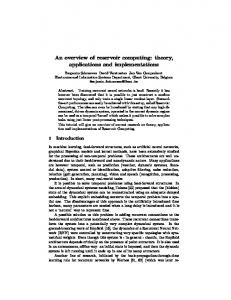
Fig. 1. General RC framework. Input X is connected to some or all of the reservoir nodes. Output Y is usually fully connected to the reservoir nodes. Only the output-weights Wout are trained.

II.

BACKGROUND

A. Reservoir Computing Feed-forward Neural Networks (NNs) are neural network models without feedback-connections, i.e. they are not aware of their own outputs [11]. They have gained popularity because of their ability to be trained to solve classification tasks. Examples include image classification [25], or playing the board game GO [22]. However, when trying to solve problems that include sequential data, such as sentence-analysis, they often fall short [11]. For example, sentences may have different lengths, and the important parts may be spatially separated even for sentences with equal semantics. Recurrent Neural Networks (RNNs) can overcome this problem [11], being able to process sequential data through memory of previous inputs which are remembered by the network. This is done by relieving the neural network of the constraint of not having feedback-connections. However, networks with recurrent connections are notoriously difficult to train by using traditional methods [2]. Reservoir Computing (RC) is a paradigm in machine learning that combines the powerful dynamics of an RNN with the trainability of a feed-forward neural network. The first

part of an RC-system consists of an untrained RNN, called reservoir. This reservoir is connected to a trained feed-forward neural network, called readout-layer. This setup can be seen in fig. 1 The field of RC has been proposed independently by two approaches, namely Echo State Networks (ESN) [13] and Liquid State Machines (LSM) [20]. By examining these approaches, important properties of reservoirs are outlined. Perhaps the most important feature is the Echo state property [13]. Previous inputs ”echo” through the reservoir for a given number of time steps after the input has occurred, and thereby slowly disappearing without being amplified. This property is achieved in traditional RC-approaches by clever reservoir design. In the case of ESN, this is achieved by scaling of the connection weights of the recurrent nodes in the reservoir [18]. As discussed in [3], the reservoir should preferably exhibit edge of chaos behaviors [16], in order to allow for high computational power [10]. B. Various RC-approaches Different RC-approaches use reservoir substrates that exhibit the desired properties. In [8] an actual bucket of water is implemented as a reservoir for speech-recognition, and in [15] the E.coli-bacteria is used as a reservoir. In [24] and more recently in [4], the usage of Random Boolean Networks (RBN) reservoirs is explored. RBNs can be considered as an abstraction of CA [9], and is thereby a related approach to the one presented in this paper.

Rule 110

0

1

1

0

1

1

1

0

011011102 = 11010

Fig. 2. Elementary CA rule 110. The figure depicts all the possible combinations that the neighbors of a cell can have. A cell is its own neighbor by convention.

binary value. This results in 28 = 256 different rules. An example of such a rule is shown in fig. 2, where rule 110 is depicted. The numbering of the rules follows the naming convention described by Wolfram [29], where the resulting binary string is converted to a base 10 number. The CA is usually updated in synchronous steps, where all the cells in the 1D-vector are updated at the same time. One update is called an iteration, and the total number of iterations is denoted by I. The rules may be divided into four qualitative classes [29], that exhibit different properties when evolved; class I: evolves to a static state, class II: evolves to a periodic structure, class III: evolves to chaotic patterns and class IV: evolves to complex patterns. Class I and II rules will fall into an attractor after a short while [16], and behave orderly. Class III rules are chaotic, which means that the organization quickly descends into randomness. Class IV rules are the most interesting ones, as they reside at a phase transition between the chaotic and ordered phase, i.e., at the edge of chaos [16]. In uniform CA, all cells share the same rule, whether non-uniform CA cells are governed by different rules. Quasi-uniform CA are nonuniform with a small number of diverse rules.

C. Cellular Automata Cellular Automaton (CA) is a computational model, first proposed by Ulam and von Neumann in the 1940s [26]. It is a complex, decentralized and highly parallel system, in which computations may emerge [23] through local interactions and without any form of centralized control. Some CA have been proved to be Turing complete [7], i.e. having all properties required for computation; that is transmission, storage and modification of information [16]. A CA usually consists of a grid of cells, each cell with a current state. The state of a cell is determined by the updatefunction f , which is a function of the neighboring states n. This update-function is applied to the CA for a given number of iterations. These neighbors are defined as a number of cells in the immediate vicinity of the cell itself. In this paper, only one-dimensional elementary CA is used. This means that the CA only consists of a one-dimensional vector of cells, named A, each cell with state S ∈ {0, 1}. In all the figures in this paper, S = 0 is shown as white, while S = 1 is shown as black. The cells have three neighbors; the cell to the left, itself, and the cell to the right. A cell is a neighbor of itself by convention. The boundary conditions at each end of the 1D-vector is usually solved by wrap-around, where the leftmost cell becomes a neighbor of the rightmost, and vice versa. The update-function f , hereafter denoted rule Z, works accordingly by taking three binary inputs, and outputting one

D. Cellular automata in reservoir computing As proposed in [30], CA may be used as reservoir of dynamical systems. The conceptual overview is shown in fig. 3. Such system is referred to as ReCA in [19], and the same name is therefore adopted in this paper. The projection of the input to the CA-reservoir can be done in two different ways [30]. If the input is binary, the projection is straightforward, where each feature dimension of the input is mapped to a cell. If the input is non-binary, the projection can be done by a weighted summation from the input to each cell. See [31] for more details. The time-evolution of the reservoir can be represented as follows: A1 = Z(A0 ) A2 = Z(A1 ) ... AI = Z(AI−1 ) Where Am is the state of the 1D CA at iteration m and Z is the CA-rule that was applied. A0 is the initial state of the CA, often an external input, as discussed later. As discussed in section II-A, a reservoir often operates at the edge of chaos [10]. Selecting CA-based reservoirs that exhibit this property is trivial, as rules that lie inside Wolfram class IV can provide this property. Additionally, to fully exploit

X P1

X PR

...

Fig. 4. The encoding used in [31]. For a total of R permutations, X is randomly mapped to vectors of the same size as the input-vector itself. X P1

X PR

...

Fig. 3. General ReCA framework. Input X is projected onto the cells of a one dimensional (1D) cellular automata, and the CA-rule is applied for a number I of iterations. In the figure, each iteration is stored, and denoted by Ai . The readout-layer weights Wout are trained according to the target-function. Figure adapted from [31]

such property, all I iterations of a the CA evolution are used for classification, and this can be stated as follows: A = [A1 ; A2 ; ...AI ] Where A is used for classification. The ReCA system must also exhibit the echo state property, as described in section II-A. This is done by allowing the CA to take external input, while still remembering the current state. As descibed in more details later, ReCA-systems address this issue by using some time-transition function, named F, which allows some previous inputs to echo through the CA. CA also provide additional advantages to RC. In [31] a speedup of 1.5-3X in the number of operations compared to the ESN [14] approach is reported. This is mainly due to a CA relying on bit-wise operations, while ESN uses floating point operations. This can be additionally exploited by utilizing custom made hardware like FPGAs. In addition, if edge-ofchaos rules are selected, Turing complete computational power is present in the reservoir. CA theoretical analysis is easier than RNNs, and they allow Boolean logic and Galois field algebra. E. ReCA system implementations ReCA systems are a very novel concept and therefore there are only few implemented examples at the current stage of research. Yilmaz [30], [31] has implemented a ReCA system with elementary CA and Game of Life [6]. Bye [5] also demonstrated a functioning ReCA-system in his master’s thesis (supervised by Nichele). The used approaches are similar, however, there are some key differences: 1) Encoding and random mappings: In the encoding stage, [31] used random permutations over the same input-vector. This encoding scheme can be seen in fig. 4. The permutation procedure is repeated R number of times, because it was experimentally observed that multiple random mappings improve performance.

Fig. 5. The encoding used in [5]. The input X is randomly mapped to a vector with size larger than the input vector itself. This mapping is done R times. The size of the vector that the input is mapped to can be determined in two ways. Either by ”automaton size”, which explicitly gives the size of the vector (in this case 8), or by the C-parameter, which the size is given by C ∗ |X pn | (in this case C=2)

In [5] a similar approach was used. The main difference is that the input is mapped to a vector that is larger than the input-vector itself. The size of this mapping-vector is given by a parameter ”automaton size”. This approach can be seen in fig. 5. The input-bits are randomly mapped to one of the bits in the mapping-vector. The ones that do not have any mapping to them are left to zero. In the work herein, the approach described in [5] is used, but with a modification. Instead of using the automaton sizeparameter, the C-parameter is introduced. The total length of the permutation is given by the number C multiplied by the length of the input-vector. In the case of fig. 5, the automation size would be 8, and C would be 2. 2) Feed-forward or recurrent: [31] proposed both a feedforward and a recurrent design. The difference was whether the whole input-sequence is presented to the system in one chunk or step-by-step. [5] only described a recurrent design. Only the recurrent architectures will be investigated in this paper. This is because it is more in line with traditional RNNs and RC-systems, and is conceptually more biologically plausible. 3) Concatenation of the encoded inputs before propagating into the reservoir: After random mappings have been created, there is another difference in the proposed approaches. In the recurrent architecture, [31] concatenates the R number of permutations into one large vector of length (R ∗ input length) before propagating it in a reservoir of the same width as this vector. The 1D input-vector at time-step t can be expressed as follows: XtP = [XtP1 ; XtP2 ; XtP3 ; ...XtPR ] XtP is inserted into the reservoir as described in section II-D, and then iterated I times. The iterations are then concatenated into the vector At , which is used for classification at time-step t.

AIt-1

Xt

Xt

AIt-1

F F F F A0t

A0t

Fig. 6. Time transition used in [31]. The sequence input Xt is combined with the state of the reservoir at the last iteration at the previous time-step At−1 . The function F may be any bit-wise function. Only one permutation I is shown in the figure to increase readability.

Fig. 7. Time-transition by permutation. The input is directly copied from Xt , according to the mapping from the encoder, as shown in fig. 5. The other cells have their values copied from the last iteration of the previous time-step At−1 . Only one permutation is shown to increase readability. I

This is relevant when discussing the computational complexity of ReCA systems. In this paper, the ”permutation transition” is used.

At = [A1 ; A2 ; ...AI ]

III. [5] adapted a different approach, the same one that was also used by the feed-forward architecture in [31], where the R different permutations are iterated in separate reservoirs, and the different reservoirs are then concatenated before they are used by the classifier. The vector which is used for classification at time-step t is as follows: At = [AtP1 ; AtP2 ; ...AtPR ] Where AtPn is the vector from the concatenated reservoir. In this paper, the recurrent architecture approach is used. 4) Time-transition: In order to allow the system to remember previous inputs, a time-transition function is needed to translate between the current time-step and the next. One possibility is to use normalized addition as time-transition function, as shown in fig. 6, with F as normalized addition. This function works as follows: The cell values are added, and if the sum is 2 (1+1) the output-value becomes 1, if the sum is 0, the output-value becomes 0 and if the sum is 1, the cell-value is decided randomly (0 or 1). The initial 1D-CAvector of the reservoir at time-step t is then expressed as: A0 = F (Xt , AI t−1 ),

t>0

Where F may be any bit-wise operation, Xt is the input from the sequential task at time-step t, and AI t−1 is the last iteration of the previous time-step. At the first time-step (t=0), the transition-function is bypassed, and the input Xt is used directly in the reservoir. Another possibility is to use ”permutation transition” as time-transition function, as seen in fig. 7. Here, all cells that have a mapping to them (from the encoder) are bit-wise filled with the value of input-vector X. If the cells do not have any mapping to them, the values from AI t−1 are inserted. This allows the CA to have memory across time-steps in sequential tasks. By adjusting the automaton-size, or C-parameter, the interaction between each time-step can be regulated. The described approaches have different effects on the parameters R and I, and also the resulting size of the reservoir.

E XPERIMENTAL S ETUP

The basic architecture implemented in this paper is shown in fig. 9. The encoder is based on the architecture described in [5]. In this paper, the parameter C is introduced as a metric on how large resulting mapping-vector should be. The concatenation procedure is adapted from [31]. The vectors, after the encoding (random mappings), are concatenated into one large vector. This vector is then propagated into the reservoir, as described in section II-E3. The time-transition function is adapted from [5]. The mappings from the encoder are saved, and used as a basis where new inputs are mapped to, as described in section II-E4. The values from the last step in the previous time-step are directly copied. The classifier used in this paper is a Support Vector Machine, as implemented in the Python machine learning framework scikit-learn [21]. The code-base that was used in this paper is available for download [1]. An example run with rule 90 is shown in fig. 8. This visualisation gives valuable insights in how the reservoir behaves when parameters are changed, and makes it easier to understand the reservoir dynamics. Most natural systems come in the form of a temporal system (sequential), i.e., an input to the system depends on previous inputs. Classical feed-forward architectures are known to have issues with temporal tasks [11]. In order to test the ReCA-system at a temporal task, the 5-bit task [12] is chosen in this paper. Such task has become a popular and widely used benchmark for reservoir computing, in particular because it tests the long-short-term memory of the system. An example data set from this task is presented in fig. 10. The length of the sequence is given by T . a1 , a2 , a3 and a4 are the input-signals, and y1 , y2 and y3 are the outputsignals. At each time-step t only one input-signal, and one output-signal, can have the value 1. The values of a1 and a2 at the first five time-steps give the pattern that the system shall learn. The next Td time-steps represent the distractor-period, where the system is distracted from the previous inputs. This is done by setting the value of a3 to 1. After the disctractor period, the a4 signal is fired which marks the cue-signal. The system is then asked to repeat the input-pattern on the outputs y1 and y2 . The output y3 is a waiting signal, which is supposed to be 1 right until the input-pattern is repeated. More details on the 5-bit memory task can be found in [14].

TABLE I.

5- BIT TASK PARAMETERS

Training set size Testing set size Distractor period No. runs

TABLE II.

32 32 200 120

CA RESERVOIR PARAMETER COMBINATIONS

CA rules I (iterations) R (random mappings) C (size multiple)

60, 90, 102, 105, 150, 153, 165, 180, 195 2, 4 4, 8 10

a combination of two rules. The tested combinations of rules are shown in table II. A. Results from the single ReCA-system

Fig. 8. Example run of the ReCA system with rule 90. The run is done with the parameters R=8, I=4 and C=5. The horizontal gray lines represent a timestep, in which the time-transition function is applied to every bit. Time flows downwards. The visualization is produced with the ReCA system described in this paper.

The results from the single reservoir ReCA-system can be seen in table III. The results in this paper are significantly better than what was reported in [5]. We can however see a similar trend. Rules 102 and 105 were able to give promising results, while rule 180 was not very well suited for this task. An exception is rule 90 and 165, where the results in table III show very high accuracy. In [31] very promising results from rule 90 are also achieved. B. Results from the parallel (non-uniform) ReCA-system

A. Use of parallel CA-reservoirs in RC In this paper the use of parallel reservoirs is proposed. The concept is shown in fig. 11. At the boundary conditions, i.e. the cell at the very end of the reservoir, the rule will treat the cell that lies within the other reservoir, as a cell in its own reservoir. This causes information/computation to flow between the reservoirs (loosely coupled). By having different rules in the reservoirs, one might be able to solve different aspects of the same problem, or even two problems at the same time. In [5], both the temporal parity and the temporal density task [14] are investigated. Which rule is most suited for a task is still an open research question. The characteristics and classes described in section II-C are useful knowledge, however it does not precisely describe why some rules perform better than others on different tasks. In fig. 12 an example run of the parallel system is showed, with rule 90 on the left, and 182 on the right. This visualization gives useful insights on how the rules interact. B. Measuring computational complexity of a CA-reservoir The size of the reservoir is crucial for the success of the system. In this paper, the reservoir size is measured by R ∗ I ∗ C. As seen in section III-A, the size of the reservoirs will remain the same both for the one-rule reservoirs and the tworule reservoirs. This is crucial in order to be able to directly compare their performances. IV.

R ESULTS

The parameters for the used 5-bit memory task can be seen in table I. The same parameters as in the single-reservoir system are used in the quasi-uniform CA reservoir system with

Results can be seen in table IV. It can be observed that combination of rules that were performing well in table III seem to give good results when combined. However, some combination of rules, e.g., 60 and 102, 153 and 195, gave worse results than the rules by themselves. We can observe the same tendencies as in the single-runs; higher R and I generally yields better results. V.

A NALYSIS

A. Single reservoir ReCA-system The complexity of the reservoir is a useful metric when comparing different approaches. If we examine rule 90, we can observe that it achieves 100% success rate at I = 4, R = 8 and C = 10. The size of the reservoir is 4 ∗ 8 ∗ 10 = 320 at this configuration. Note that even though lower values of R and I also give 100%, at R = 4 and I = 4 the success is 97.5%, yet again 100% at I = 4 and R = 8. [31] reported a 100% success-rate on the same task with R = 32 and I = 16. The C-parameter was set to 1. As such, the size of the reservoir is 32 ∗ 16 ∗ 1 = 512 (feed-forward architecture). [31] also presented results on the 5-bit task using the recurrent architecture. 100% success-rate was achieved with I = 32 TABLE III. Rule 60 90 102 105 150 153 165 180 195

S INGLE RESERVOIR CA ON 5- BIT TASK . S UCCESSFUL RUNS WITH T=200 I=2, R=4 25.8% 100.0% 30.8% 95.8% 96.7% 26.7% 100.0% 9.2% 39.2%

I=2, R=8 53.3% 100.0% 63.3% 99.2% 100.0% 55.0% 100.0% 38.3% 61.7%

I=4, R=4 76.7% 97.5% 71.7% 99.2% 100.0% 80.0% 100.0% 0.8% 79.2%

I=4, R=8 95.0% 100.0% 96.7% 100.0% 100.0% 95.0% 100.0% 1.7% 95.8%

Time-step 1 X0

Encoder, R=2, C=2

X0P1

X0P2

concatenation X0P A1 A2

A(1)

Classifier

A3 A4

AI = A4

Time-step 2 X1

Encoder, R=2, C=2

X1P1

X1P2

concatenation X1P

Time-transition

A1 A2 A3

A(2)

Classifier

A4

AI = A4

Fig. 9. Architecture of the implemented system. The encoding is done according to the encoding-scheme as shown in fig. 5, but with the slight modification of the C-parameter. The encoding is exemplified with R=2 and C=2, which yields a size of eight for each permutation. The two permutations are then concatenated. At time-step 1, there are no previous inputs, and the concatenated vector is simply used as the first iteration of the CA-reservoir. The rule Z is then applied for I iterations. At time-step 2, the encoding and concatenation is repeated. The time-transition scheme is then applied, as described in fig. 7. The procedure as described in time-step 2 is repeated until the end of the sequence.

a1a2a3a4y1y2y3

0100 001 X1 0100 001 1000 001 0100 001 1000 001 0010 001 0010 001 ... 0010 001 Time 0010 001 0001 001 0010 010 0010 010 0010 100 0010 010 XT 0010 100 X0

...

Learn pattern (5)

Distractor (Td) Cue (1)

Repeat pattern (5)

...

Fig. 10. Example data from the 5-bit task. The length of the sequence is T . The signals a1 , a2 , a3 and a4 are input-signals, while y1 , y2 and y3 are output-signals. In the first five time-steps the system learns the pattern. The system is then distracted for Td time-steps. After the cue-signal is set, the system is expected to reproduce the pattern that was learned. Input

RULE A

Fig. 12. Example run of the ReCA system with rule 90 on the left and 182 on the right. Information is allowed to flow between the reservoirs. The run is done with the parameters R=8, I=4 and C=5. The horizontal gray lines represent a time-step, in which the time-transition function is applied to every bit. Time flows downwards. The visualization is produced with the implemented system.

RULE B

TABLE IV.

I

Output

Fig. 11. Concept behind parallel CA reservoirs. Iterations flow downward. The rules are interacting at the middle boundaries and at the side boundaries, where the CA wraps around.

and R = 45. This yields a reservoir size of 32 ∗ 45 = 1440. Those results were intended to study the relationship between the distractor period of the 5-bit task, and the R number of random mappings. The I was kept fixed at 32 during this experiment. Even if the motivation for the experiments were different, the comparison of results gives insight that the reservoir size itself may not be the only factor that determines the performance of the ReCA system. B. Parallel reservoir (non-uniform) ReCA-system Why are some combinations better than others? As observed in section IV-B, rules that are paired with others rules that perform well on their own, also perform well together. The combination of rule 90 and rule 165 is observed to be very successful. As described in [28], rule 165 is the complement of rule 90. If we observe the single-CA results in table III we can see that rule 90 and 165 perform very similarly. Examining one of the worst-performing rule-combinations

PARALLEL CA ON 5- BIT TASK . S UCCESSFUL RUNS WITH T=200

Rule 60 and 90 60 and 102 60 and 105 60 and 150 60 and 153 60 and 165 60 and 180 60 and 195 90 and 102 90 and 105 90 and 150 90 and 153 90 and 165 90 and 180 90 and 195 102 and 105 102 and 150 102 and 153 102 and 165 102 and 180 102 and 195 105 and 150 105 and 153 105 and 165 105 and 180 105 and 195 150 and 153 150 and 165 150 and 180 150 and 195 153 and 165 153 and 180 153 and 195 165 and 180 165 and 195 180 and 195

I=2, R=4 87.5% 0.0% 81.2% 71.9% 0.0% 87.5% 43.8% 0.0% 90.6% 100.0% 100.0% 93.8% 90.6% 90.6% 87.5% 78.1% 81.2% 0.0% 93.8% 0.0% 0.0% 93.8% 75.0% 96.9% 93.8% 65.6% 87.5% 100.0% 81.2% 78.1% 81.2% 3.1% 0.0% 96.9% 87.5% 40.6%

I=2, R=8 100.0% 0.0% 100.0% 100.0% 0.0% 93.8% 53.1% 0.0% 100.0% 100.0% 100.0% 96.9% 100.0% 100.0% 96.9% 100.0% 100.0% 0.0% 100.0% 40.6% 0.0% 100.0% 93.8% 100.0% 100.0% 93.8% 100.0% 100.0% 100.0% 96.9% 100.0% 46.9% 0.0% 96.9% 100.0% 87.5%

I=4, R=4 96.9% 0.0% 96.9% 96.9% 0.0% 96.9% 90.6% 0.0% 100.0% 100.0% 100.0% 96.9% 100.0% 100.0% 100.0% 96.9% 96.9% 0.0% 100.0% 3.1% 0.0% 100.0% 93.8% 100.0% 100.0% 96.9% 96.9% 100.0% 100.0% 100.0% 100.0% 0.0% 0.0% 100.0% 100.0% 93.8%

I=4, R=8 100.0% 0.0% 100.0% 100.0% 0.0% 96.9% 84.4% 0.0% 96.9% 100.0% 100.0% 100.0% 100.0% 100.0% 100.0% 100.0% 100.0% 3.1% 100.0% 6.2% 3.1% 100.0% 100.0% 100.0% 100.0% 100.0% 100.0% 100.0% 100.0% 100.0% 100.0% 0.0% 0.0% 100.0% 100.0% 96.9%

Ideally, the usage of more than two different rules could prove a powerful tool. The rule space would then grow even larger, and an exhaustive search would be infeasible. However, one possibility would be to use evolutionary algorithms to search for suitable rules. Adding more and more rules would bring the reservoir closer to a true non-uniform CA. In [14] a wide range of different tasks is presented. In this paper only one (5-bit task) is used as a benchmark. By combining different rules’ computational power, one could design a reservoir that performs well on a variety of tasks.

R EFERENCES

Fig. 13. Example run of the ReCA system with rule 153 and 195. The run is done with the parameters R=8, I=4 and C=5. The horizontal gray lines represent a time-step, in which the time-transition function is applied to every bit. Time flows downwards. The visualization is produced with the implemented system.

of the experiments, i.e., rule 153 and rule 195, we get some useful insight as seen in fig. 13. Here it is possible to notice that the interaction of rules creates a ”black” region in the middle (between the rules), thereby effectively reducing the size of the reservoir. As described in [27], rule 153 and 192 are the mirrored complements. Rule 105 is an interesting rule to be combined with others. As described in [29], the rule does not have any compliments or any mirrored compliments. Nevertheless, as seen in table IV-B, it performs well in combination with most other rules. VI.

C ONCLUSION

A framework for using cellular automata in reservoir computing has been implemented, which makes use of uniform CA and quasi-uniform CA. Relationship between reservoir size and performances of the system are presented. The implemented configuration using parallel CA reservoir is tested in this paper for the first time (to the best of the authors’ knowledge). Results have shown that some CA rules work better in combination than other. Good combinations tend to have some relation, e.g. being complementary. Rules that are mirrored compliments do not work well together, because they effectively reduce the size of the reservoir. The concept is still very novel, and a lot of research is left to be done, both regarding the use of non-uniform CA reservoir, as well as ReCA-systems in general. As previously discussed, finding the best combination of rules is not trivial. If we only consider the usage of two distinct rules, the rule space grows from only 256 single256! = 32640 different combinations. reservoir options to 2!∗254! Matching two rules that perform well together can be quite a challenge. By investigating the characteristics of the rules, e.g., with lambda-parameter [16], Lyapunov exponent [17] or other metrics, it may be possible to pinpoint promising rules.

[1]

Repository of the implemented reca system used in this paper. https: //github.com/magnusgundersen/spec. Accessed: 2016-12-14.

[2]

Yoshua Bengio, Patrice Simard, and Paolo Frasconi. Learning longterm dependencies with gradient descent is difficult. IEEE transactions on neural networks, 5(2):157–166, 1994.

[3]

Nils Bertschinger and Thomas Natschl¨ager. Real-time computation at the edge of chaos in recurrent neural networks. Neural computation, 16(7):1413–1436, 2004.

[4]

Aleksander Vognild Burkow. Exploring physical reservoir computing using random boolean networks. Master’s thesis, NTNU, 2016.

[5]

Emil Taylor Bye. Investigation of elementary cellular automata for reservoir computing. Master’s thesis, NTNU, 2016.

[6]

John Conway. The game of life. Scientific American, 223(4):4, 1970.

[7]

Matthew Cook. Universality in elementary cellular automata. Complex systems, 15(1):1–40, 2004.

[8]

Chrisantha Fernando and Sampsa Sojakka. Pattern recognition in a bucket. In European Conference on Artificial Life, pages 588–597. Springer, 2003.

[9]

Carlos Gershenson. Introduction to random boolean networks. arXiv preprint nlin/0408006, 2004.

[10]

Thomas E Gibbons. Unifying quality metrics for reservoir networks. In Neural Networks (IJCNN), The 2010 International Joint Conference on, pages 1–7. IEEE, 2010.

[11]

Ian Goodfellow, Yoshua Bengio, and Aaron Courville. Deep learning. Book in preparation for MIT Press, 2016.

[12]

Sepp Hochreiter and J¨urgen Schmidhuber. Long short-term memory. Neural computation, 9(8):1735–1780, 1997.

[13]

Herbert Jaeger. The echo state approach to analysing and training recurrent neural networks-with an erratum note. Bonn, Germany: German National Research Center for Information Technology GMD Technical Report, 148:34, 2001.

[14]

Herbert Jaeger. Long short-term memory in echo state networks: Details of a simulation study. Technical report, Jacobs University Bremen, 2012.

[15]

Ben Jones, Dov Stekel, Jon Rowe, and Chrisantha Fernando. Is there a liquid state machine in the bacterium escherichia coli? In 2007 IEEE Symposium on Artificial Life, pages 187–191. Ieee, 2007.

[16]

Chris G Langton. Computation at the edge of chaos: phase transitions and emergent computation. Physica D: Nonlinear Phenomena, 42(1):12–37, 1990.

[17]

Robert Legenstein and Wolfgang Maass. Edge of chaos and prediction of computational performance for neural circuit models. Neural Networks, 20(3):323–334, 2007.

[18]

Mantas Lukoˇseviˇcius, Herbert Jaeger, and Benjamin Schrauwen. Reservoir computing trends. KI-K¨unstliche Intelligenz, 26(4):365–371, 2012.

[19]

Mrwan Margem and Ozg¨ur Yilmaz. An experimental study on cellular automata reservoir in pathological sequence learning tasks. 2016.

[20]

Thomas Natschl¨ager, Wolfgang Maass, and Henry Markram. The” liquid computer”: A novel strategy for real-time computing on time series. Special issue on Foundations of Information Processing of Telematik, 8(Lnmc-Article-2002-005):39–43, 2002.

[21]

[22]

[23] [24]

[25]

[26] [27] [28] [29] [30] [31]

Fabian Pedregosa, Ga¨el Varoquaux, Alexandre Gramfort, Vincent Michel, Bertrand Thirion, Olivier Grisel, Mathieu Blondel, Peter Prettenhofer, Ron Weiss, Vincent Dubourg, et al. Scikit-learn: Machine learning in python. Journal of Machine Learning Research, 12(Oct):2825–2830, 2011. David Silver, Aja Huang, Chris J Maddison, Arthur Guez, Laurent Sifre, George Van Den Driessche, Julian Schrittwieser, Ioannis Antonoglou, Veda Panneershelvam, Marc Lanctot, et al. Mastering the game of go with deep neural networks and tree search. Nature, 529(7587):484–489, 2016. Moshe Sipper. The emergence of cellular computing. Computer, 32(7):18–26, 1999. David Snyder, Alireza Goudarzi, and Christof Teuscher. Computational capabilities of random automata networks for reservoir computing. Physical Review E, 87(4):042808, 2013. Christian Szegedy, Wei Liu, Yangqing Jia, Pierre Sermanet, Scott Reed, Dragomir Anguelov, Dumitru Erhan, Vincent Vanhoucke, and Andrew Rabinovich. Going deeper with convolutions. In Proceedings of the IEEE Conference on Computer Vision and Pattern Recognition, pages 1–9, 2015. John Von Neumann, Arthur W Burks, et al. Theory of self-reproducing automata. IEEE Transactions on Neural Networks, 5(1):3–14, 1966. Eric W Weisstein. ”rule 60.” from mathworld – a wolfram web resource. http://mathworld.wolfram.com/Rule60.html. Accessed: 2016-12-10. Eric W Weisstein. ”rule 90.” from mathworld – a wolfram web resource. http://mathworld.wolfram.com/Rule90.html. Accessed: 2016-12-10. Stephen Wolfram. A new kind of science, volume 5. Wolfram media Champaign, 2002. Ozgur Yilmaz. Reservoir computing using cellular automata. arXiv preprint arXiv:1410.0162, 2014. Ozgur Yilmaz. Connectionist-symbolic machine intelligence using cellular automata based reservoir-hyperdimensional computing. arXiv preprint arXiv:1503.00851, 2015.