Abstract. A Pearson residual is defined as a residual between an observed value and expected one of each cell in a contingency table, which measures the ...
International Journal of Computational Intelligence Systems, Vol. 4, No. 5 (September, 2011), 1080-1089
Residual as Linear Sum of Matrix Determinants in Multiway Contingency Tables Shusaku Tsumoto and Shoji Hirano Department of Medical Informatics, Faculty of Medicine, Shimane University 89-1 Enya-cho Izumo 693-8501 Japan E-mail: {tsumoto,hirano}@med.shimane-u.ac.jp
Abstract A Pearson residual is defined as a residual between an observed value and expected one of each cell in a contingency table, which measures the degree of statistical dependence of two attribute-value pairs corresponding to the cell. This paper shows that this residual is decomposed into a linear sum of determinants of 2 × 2 subtables, which means that the geometrical nature of the residuals can be viewed from grasmmanian algebra. Keywords: Pearson Residual, Determinants, Multiway Contingency Table, Information Granules
1.
Introduction
Statistical independence between two attributes is a very important concept in data mining and statistics. The definition P(A, B) = P(A)P(B) show that the joint probability of A and B is the product of both probabilities. This gives several useful formula, such as P(A|B) = P(A), P(B|A) = P(B). In a data mining context, these formulae show that these two attributes may not be correlated with each other. Thus, when A or B is a classification target, the other attribute may not play an important role in its classification. Although independence is a very important concept, it has not been fully and formally investigated as a relation between two attributes. In this paper, a statistical independence in a contingency table is focused on from the viewpoint of granular computing and linear algebra, which is continuation of studies on contingency matrix
theory2,4,6,5 . Tsumoto2,5 discusses that a contingency table compares two attributes with respect to information granularity and shows that statistifcal independence in a contingency table is a special form of linear depedence of two attributes. Especially, when the table is viewed as a matrix, the above discussion shows that the rank of the matrix is equal to 1.0. Tsumoto4 matrix algebra is a key point of analysis of this table. A contingency table can be viewed as a matrix and several operations and ideas of matrix theory are introduced into the analysis of the contingency table. On the other hand, in another paper6 , Tsumoto shows that the Pearson residual of a contingency matrix is represented as a linear sum of 2 × 2 submatrices, whose number is equal to the degree of freedom. In this paper, we extend residual analysis to multidimensional cases. The results show that multidimensional residuals are also represented as a linear
Published by Atlantis Press Copyright: the authors 1080
sum of determinants of 2 × 2 submatrices, the number of which is equal to the degree of freedom in a given contingency table. Furthermore, the sum includes several kinds of units for statistical independence/dependence, such as total independence and partial independence. This also suggests that 2 × 2 submatrices in a multidimensional data cube can be viewed as information granules for measuring statistical dependence. The paper is organized as follows: Section 2 discusses the characteristics of contingency tables. Section 3 shows the conditions on statistical independence for contingency tables. Section 4 gives the results of residual analysis of multiway contingency tables. Section 5 illustrates the nature of residuals of multiway tables by using several samples. Section 6 shows that the number of the determinants of 2 × 2 submatrices is exactly the same as the degree of freedom in a three-way contingency table. Finally, Section 7 concludes this paper.
where their marginal sums are not included as elements. For simplicity, if we do not need to specify R1 and R2 , we use M(m, n, N) as a contingency matrix with m rows, n columns and N samples. One of the important observations from granular computing is that a contingency table shows the counting relations between two attributes with respect to intersection of their supporting sets. When two attributes have different numbers of equivalence classes, the situation may be a little complicated. But, in this case, due to knowledge about linear algebra, we only have to consider an attribute which has a smaller number of equivalence classes. and the surplus number of equivalence classes of the attributes with larger number of equivalnce classes can be projected into the other partitions. In other words, a m × n matrix or contingency table includes a projection from one attributes to the other one. 3.
2.
Multiway Contingency Table
Definition 1. Let R1 , R2 , · · · , Rn denote n(∈ N) multinominal attributes in an attribute space A which have m1 , m2 , · · · , mn values Let |R j = A ji | denote the set of data whose jth-attribute is equal to A ji (ith-partition of j). A contingency table T (R1 , R2 , · · · , Rn ) is a table, each of whose cells can be defined as:
Statistical Independence in Multi-way Contingency Tables
Let us consider a m × n contingency table shown in Table 1. Statistical independence of R1 and R2 gives the following formulae: P([R1 = Ai , R2 = B j ]) = P([R1 = Ai ])P([R2 = B j ]) (i = 1, · · · , m, j = 1, · · · , n). According to the definition of the table, xi j ∑n xik ∑m xl j = k=1 × l=1 . N N N
xi1 i2 ···in = #{x ∈ |R1 = Ai1 | ∧ |R2 = Ai2 | · · · ∧ |Rn = Ain |}, with these marginal sums. For example, in the two dimensional case, this table is arranged into the form shown in Table 1, where: |[R1 = A j ]A | = ∑m i=1 x1i = x· j , |[R2 = Bi ]A | = ∑nj=1 x ji = xi· , |[R1 = A j ∧ R2 = Bi ]A | = xi j , |U| = N = x·· (i = 1, 2, 3, · · · , n and j = 1, 2, 3, · · · , m). Definition 2. A multiway contigency matrix MR1 ,R2 ,··· ,Rn (N) is defined as: which is composed of
(1)
Thus, we have obtained: xi j =
∑nk=1 xik × ∑m l=1 xl j . N
Thus, for a fixed j, xia j ∑n xi k = nk=1 a xib j ∑k=1 xib k In the same way, for a fixed i,
xi1 i2 ···in = #{x ∈ |R1 = Ai1 | ∧ |R2 = Ai2 | · · · ∧ |Rn = Ain |}, Published by Atlantis Press 2 Copyright: the authors 1081
xi ja ∑m l=1 xl ja = m xi jb ∑l=1 xl jb
(2)
Table 1: Contingency Table (m × n) A1 A2 · · · An Sum B1 x11 x12 · · · x1n x1· B2 x21 x22 · · · x2n x2· ··· ··· ··· ··· ··· ··· Bm xm1 xm2 · · · xmn xm· Sum x·1 x·2 · · · x·n x·· = N
Since this relation will hold for any j, the following equation is obtained: xia 1 xia 2 xi n ∑n xia k . = · · · = a = k=1 xib 1 xib 2 xib n ∑nk=1 xib k
(3)
xi j =
Theorem 1. If two attributes in a contingency table shown in Table 1 are statistical indepedent, the following equations hold:
Or Thus, statistical independence can be viewed as the specific relations between assignments of i, j and “·”. By use of the above relation, Equation (4) can be rewritten as: xi1 j xi • = 1 , xi2 j xi2 •
(4)
where the right hand side gives the ratio of marginal column sums. Equation (7) can be extended into multivariate cases. Let us consider a three attribute case. Statistical independence with three attributes is defined as:
for all rows: ia and ib (ia , ib = 1, 2, · · · , m).
3.1. Three-way Table Let “•” denote as the sum over the row or column of a contingency matrix. That is , n
xi• =
∑ xi j
(5)
∑ xi j ,
(6)
xi jk xi•• x• j• x••k = × × , x••• x••• x••• x•••
(8)
2 xi jk x••• = xi•• x• j• x••k ,
(9)
Thus,
j=1 m
x• j =
xi• × x• j x••
xi j x•• = xi• x• j
Since the right hand side of the above equation will be constant, thus all the ratios are constant. Thus,
xia 1 xia 2 xi n = · · · = a = const. xib 1 xib 2 xib n
That is,
which corresponds to:
i=1
where (5) and (6) shows marginal column and row sums. Then, it is easy to see that
P(A = a, B = b,C = c) = P(A = a)P(B = b)P(C = c), (10)
x•• = N, where N denotes the sample size. Then, Equation (2) is reformulated as: xi j xi• x• j = × x•• x•• x••
(7)
where A,B,C correspond to the names of attributes for i, j,k, respectively. In the statistical context, statistical independence requires a hiearchical model. That is, statistical independence of three attributes requires that all the
Published by Atlantis Press 3 Copyright: the authors 1082
two pairs of three attributes should satisfy the equations of statistical independence. Thus, for Equation (10), the following equations should satisfy: P(A = a, B = b) = P(A = a)P(B = b), P(B = b,C = c) = P(B = b)P(C = c), and P(A = a,C = c) = P(A = a)P(C = c).
x••ka x••kb x• ja • x• jb • xia •• xib ••
for all i, j, and k.
Thus, xi j• x••• = xi•• x• j• xi•k x••• = xi•• x••k x• jk x••• = x• j• x••k
(11) (12) (13)
xi jk x••• = xi j• x••k , xi jk x••k = xi j• x•••
(14)
In the same way, the following equations are obtained: xi jk xi•k xi jk x• jk
= =
x• j• x••• xi•• x•••
= =
n−1 xi1 i2 ···in × x••···•
= xi1 •···• x•i2 ···• × · · · × x••···ik ···• × · · · × x••···•in
(16)
Theorem 2. If a three-way contingency table satisfy statistical independence, then the following three equations should be satisfied: =
Theorem 4. If a m-way contingency table satisfy statistical independence, then the following equation should be satisfied for any k-th attribute ik and jk (k = 1, 2, · · · , n) where n is the number of attributes. x••···ik ···• xi1 i2 ···ik ···in = xi1 i2 ··· jk ···in x••··· jk ···• Also, the following equation should be satisfied for any ik :
(15)
In summary, the following theorem is obtained.
xi jk xi j• xi jk xi•k xi jk x• jk
3.2. Multi-way Table The above discussion can be easily extedned into a multi-way contingency table.
From Equation (9) and Equation (11),
Therefore,
following equations hold: xi jka = xi jkb xi ja k = xi jb k xia jk = xib jk
Thus, a Pearson residual, a difference between an observed value for each cell in a contingency table and an expected value, is defined as: σi1 i2 ···in = xi1 i2 ···in xi •···• × · · · × x••···ik ···• × · · · × x••···•in − 1 n−1 x••···• (17)
x••k x••• x• j• x••• xi•• x•••
4.
Thus, the equations corresponding to Theorem 1 are obtained as follows. Corollary 3. If three attributes in a contingency table shown in Table 1 are statistical indepedent, the
Information Granule for Contingency Matrices
4.1. Residual of Contingency Matrices Tsumoto and Hirano 3,6 discusses the meaning of pearson residuals from the viewpoint of linear algebra.
Published by Atlantis Press 4 Copyright: the authors 1083
From Equation (17), the residual is defined as: xi• × x• j . σi j = xi j − x••
are obtained. σ11 = σ12 =
And simple calculation leads to the following theorem. Theorem 5. The residual σi j of two-dimensional contigency matrix is obtained as: σi j = =
1 � xi j x•• − xi• × x• j x•• ( ! 1 xi j ∑ ∑ xkl − ∑ xil x•• l6= j k6=i l6= j
=
1 (xi j xkl − xk j xil ) x•• k6∑ =i
=
1 ∆i,k,lj , x•• k6∑ =i
!)
∑ xk j
k6=i
l6= j
l6= j
where ∆i,k,lj is the determinant of a 2 × 2 submatrix of the original contingency matrix with selection of i and k rows and j and l columns. Also, the sum takes over k = m and l = n. Equivalently, the above formula can be represented as: σi j x•• = ∑ ∆i,k,lj ,
σ21 = σ22 =
� 1 � 1,1 1,1 1,1 ∆2,2 + ∆1,1 + ∆ + ∆ 2,3 3,2 3,3 x·· � � 1 1,2 1,2 1,2 ∆1,2 + ∆ + ∆ + ∆ 2,3 3,1 3,3 x·· 2,1 � � 1 2,1 2,1 2,1 ∆2,1 + ∆ + ∆ + ∆ 1,3 3,2 3,3 x·· 1,2 � � 1 2,2 2,2 2,2 ∆2,2 1,1 + ∆1,3 + ∆3,1 + ∆3,3 x··
As shown in the above formulae, the number of the subderminants in σi j is equal to (3 − 1) ∗ (3 − 1) = 4, the degree of freedom of 3 × 3 contingency table. Thus, a 2 × 2 submatrix in a contingency table can be viewed as a information granule for statistical (in)dependence. Furthermore, the number of granules is equal to the degree of freedom of the table. Can we generalize these results into statistical independence of multivariate cases ? This question is answered in this paper as follows.
4.2. Information Granule for Three-way Contingency Tables The residual for xi jk is defined as: σi jk = xi jk −
k6=i l6= j
xi•• × x• j• × x••k . 2 x•••
(18)
Here, we define “partial residuals” in which one of three attributes are summarized (marginalized) as follows:
where the sum takes over k = m andl = n.
Especially, for m = n = 2, the residual is equal to the determinant of the original matrix. σi j x•• = ∆i,k,lj ,
(19)
σi•k
(20)
σi j• where k 6= i and l 6= j. Thus, σ11 x•• = ∆1,1 2,2 , In the case of 3×3 tables, the following formulas
x• j• × x••k x••• xi•• × x••k = xi•k − x••• xi•• × x• j• = xi j• − x•••
σ• jk = x• jk −
(21)
Then, by using (19), the residual (18) is refor-
Published by Atlantis Press 5 Copyright: the authors 1084
mualted as: xi•• × x• j• × x••k 2 x••• xi•• x• j• x••k xi jk − x••• x••• � xi•• x• jk − σ• jk xi jk − x••• xi•• xi•• σ• jk + xi jk − x• jk x••• x••• xi•• σ• jk x••• � 1 + xi jk x••• − xi•• x• jk x•••
the other hand, the last part is different from the former two sums. This sum is zero if the conditional independence are satisfied, that is, if xi jk = xi•• x• jk , whose meaning is i and j are statistical independence with k fixed. Thus, the following theorem is obtained.
σi jk = xi jk − = = = =
Theorem 6. The residual of three-dimensional contingency table is decomposed as: σi jk = =
(22)
Since σ• jk is equivalent to the residual of twodimensional contigency matrix, it can be represented as a linear sum of 2 × 2 submatrices. Thus, the latter part xi jk x••• − xi•• x• jk should be examined. Let us denote this part by σ ijk .
xi•• σ• jk + σ ijk x••• xi•• σ• jk x••• +
1 ik ∑ ∆( j)ln +
x•••
l6=i n6=k
∑ ∆(k)ilmj
l6=i m6= j
+
∑
l6=i m6= j n6=k
σ ijk = xi jk x••• − xi•• x• jk !
� xi jk xlmn − ximn xl jk .
(24)
= xi jk xi•• + ∑ xl•• l6=i
! 4.3. Information Granule for Multi-way Contingency Table
−xi•• xi jk + ∑ xm jk m6=i
= xi jk ∑ xl•• − xi•• ∑ xm jk l6=i
=
xi jk xl•• − xi•• xl jk
∑
The structure of Equation (24) suggests that the residual can be defined in a recursive way.
m6=i
�
Theorem 7. Let n be a number of attributes in a contingency table ( i.e. n-way contingency table. The residual of the cell(i1 , i2 , · · · , ın ), σi1 i2 ···in is decomposed as follows.
l6=i
=
∑
xi jk xlmn − ximn xl jk
�
l6=i m6= j or n6=k
=
∑ ∆( j)ikln + ∑ ∆(k)ilmj
l6=i n6=k
+
∑
l6=i m6= j
� xi jk xlmn − ximn xl jk ,
σi1 i2 ···in (23)
= =
l6=i m6= j n6=k
+
where ∆( j)ik ln denotes the determinant of 2 × 2 matrix in which i and l rows and k and n columns are selected with m = j fixed and ∆(k)ilmj denotes the determinant of 2 × 2 matrix in which i and l rows and j and m columns are selected with n = k fixed. On
xi1 •···• 1 σ•i2 ···in + σ i1 x••···• x••···• i2 ···in xi1 •···• σ•i ···i x••···• 2 n 1 (xi i ···i x••···• − xi1 ••• x•i2 ···in ) , x••···• 1 2 n (25)
For example, in the case of a four-dimensional contingency table, a residual σi1 i2 i3 i4 is decomposed
Published by Atlantis Press 6 Copyright: the authors 1085
as: =
σi1 i2 i3 i4
= +
xi1 ••• 1 σ•i i i + σ i1 x•••• 2 3 4 x•••• i2 i3 i4 xi1 ••• σ•i i i x•••• 2 3 4 1 (xi i i i x•••• − xi1 ••• x•i2 i3 i4 ) , x•••• 1 2 3 4
where σ•i2 i3 i4 can be decomposed as shown in Equation (24): =
σ•i2 i3 i4
= +
x•i2 •• 1 σ••i3 i4 + σ i2 x•••• x•••• •i3 i4 x•i2 •• σ••i3 i4 x•••• 1 (x•i2 i3 i4 x•••• − x•i2 •• x••i3 i4 ) . x••••
Then, σ•ii23 i4 is reformulated as shown in Equation (23). 5.
analysis 1 . This result is not accidental, as shown in Section 6. 1 can be deThe geometrical structure of σ11 picted as Figure 1. The shadowed parts correspond to x111 x212 − x211 x112 , x111 x222 − x211 x112 , and x111 x221 −x211 x121 . Thus, these three parts give three possible combinations of parallelograms which has x111 x211 as the fixed edge. 5.2. 3 × 2 × 3 Contingency Table The residual of a cell (1, 1, 1) is decomposed as: σ111 = = and 1 σ11 = (x111 x212 − x211 x112 ) +(x111 x213 − x211 x113 ) +(x111 x221 − x211 x121 ) +(x111 x222 − x211 x122 ) +(x111 x223 − x211 x123 ) +(x111 x231 − x211 x131 ) +(x111 x232 − x211 x132 ) +(x111 x233 − x211 x133 )
Examples
5.1. 2 × 2 × 2 Contingency Table The residual of a cell (1, 1, 1) is decomposed as: σ111 = =
x1•• 1 σ•11 + (x111 x••• − x1•• x•11 ) x••• x••• x1•• 1 1 σ•11 + σ x••• x••• 11
and 1 σ11 = (x111 x212 − x211 x112 ) + (x111 x221 − x211 x121 ) + (x111 x222 − x211 x112 ),
which consists of three components. Since the number of determinants of σ•11 is equal to 1 and that of 1 is equal to 3, the total number of the determiσ11 nants is equal to 4. In the case of conditional inde1 is equal pendence xi jk = xi•• x• jk , the last part of σ11 to 0, the total number of the derminants in the residual is equal to 3. It is notable that these numbers on the degree of freedom are exactly the same as those of the degree of freedom in contingency table
1 x1•• σ•11 + (x111 x••• − x1•• x•11 ) x••• x••• x1•• 1 1 σ•11 + σ x••• x••• 11
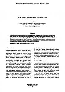
which consists of eight components. The geometri1 can be depicted as Figure 2. The cal structure of σ11 shadowed parts correspond to x111 x212 − x211 x112 , x111 x213 − x211 x113 , x111 x221 − x211 x121 , x111 x222 − x211 x122 , x111 x223 − x211 x123 , x111 x231 − x211 x131 , x111 x232 − x211 x132 , and x111 x233 − x211 x133 . Thus, these eight parts give eight possible combinations of parallelograms which has x111 x211 as the fixed edge. 5.3. 3 × 3 × 3 Contingency Table The residual of a cell (1, 1, 1) is decomposed as: σ111 = =
Published by Atlantis Press 7 Copyright: the authors 1086
x1•• 1 σ•11 + (x111 x••• − x1•• x•11 ) x••• x••• x1•• 1 1 σ•11 + σ x••• x••• 11
x111
x121 x221
x211
x112
x122
x212
x222
Figure 1: Geometrical Structure of 2 × 2 × 2 Contingency Table 6.
and 1 σ11 = (x111 x212 − x211 x112 ) +(x111 x213 − x211 x113 ) +(x111 x221 − x211 x121 ) +(x111 x222 − x211 x122 ) +(x111 x223 − x211 x123 +(x111 x231 − x211 x131 ) +(x111 x232 − x211 x132 ) +(x111 x233 − x211 x133 ) +(x111 x312 − x311 x112 ) +(x111 x313 − x311 x113 ) +(x111 x321 − x311 x121 ) +(x111 x322 − x311 x122 ) +(x111 x323 − x311 x123 ) +(x111 x331 − x311 x131 ) +(x111 x332 − x311 x132 ) +(x111 x333 − x311 x133 )
Discussion
6.1. #Degreee of Freedom = #Information Granules In the above sections, we mentioned that the number of derminants of 2 × 2 submatrices in a threeway contingency table is equal to the degree of freedom of χ 2 test statistic in contingency table analysis. This section shows that it is not accidental. Everitt 1 shows that the degree of freedom of χ 2 test statistic is given as: d. f . = rcl − (r − 1) − (c − 1) − (l − 1) − 1 = rcl − r − c − l + 2 (26) On the other hand, with the hypothesis of conditional independence on (r − 1) row probabilities and column × layer probabilities (cl − 1), the degree of freedom is given as: d. f . = rcl − (cl − 1) − (r − 1) − 1 = rcl − cl − r + 1
which consists of 16 components. The geometri1 can be depicted as Figure 3. cal structure of σ11 In the same way as 2 × 3 × 3 table, these 16 parts give all the combinations of parallelograms which has x111 x211 and x111 x311 as the fixed edges.
(27)
Let us go back to Equation 25 in Theorem 6 and assume that indices i, j, and k correspond to row, column, and layer, respectively. The numbers of the derminants are summarized into:
Published by Atlantis Press 8 Copyright: the authors 1087
x111
x121
x211
x221
x131 x231
x122
x112
x132
x212
x232
x222
x133 x113 x213
x123 x223
x233
Figure 2: Geometrical Structure of 2 × 3 × 3 Contingency Table σ• jk (c − 1)(l − 1) ∆( j)ik (r − 1)(l − 1) ln ij ∆(k)lm (r − 1)(c − 1) xi jk xlmn − ximn xl jk (r − 1)(c − 1)(l − 1) The total number of the determinants sum is: sum = (c − 1)(l − 1) + (r − 1)(l − 1) +(r − 1)(c − 1) + (r − 1)(c − 1)(l − 1) = rcl − r − c − l + 2, which is equal to Equation 26. Thus, the following theorem is obtaied. Theorem 8. The total number of derminants of 2 × 2 submatrices in a three-way contingency table is equal to the degree of freedom of χ 2 test statistic in contingency table analysis. Furthermore, since the total number of the derminants of two-way contingency tables with c rows and l columns is (c − 1)(l − 1), the difference between the number of the determinants of three-way tables and that of two tables, δ is equal to: δ
= (c − 1)(l − 1) + (r − 1)(l − 1) +(r − 1)(c − 1) + (r − 1)(c − 1)(l − 1) −(c − 1)(l − 1) = rcl − cl − r + 1,
which is equal to Equation 27. Thus, Theorem 9. The total number of derminants of 2 × 2 submatrices in a three-way contingency table can be decomposed into the sum of the total number of derminants in a two-way contingency table and that in a three-way contingency table with conditional independence. It will be our future work to generalize these results into multi-way contingency tables, whose dimension is larger than 4. 6.2. Towards Applications Since the determinants of 2 × 2 subtables (submatrices) can be viewed as information granules, these values measure the local nature of a given table. On the other hand, a χ 2 -test statistic gives the global nature of a given table. If we only need to evaluate the global degree of statistical independence, a chi2 test statistic is sufficient. However, when we want to evalute the precise nature of a given table, or the local degree of statistical independence, the values for each subtable will play important roles in further investigation of the local relations between attributes. In other words, information granules give local natures of statistical independence and those behavior is integrated into the global nature of a given ta-
Published by Atlantis Press 9 Copyright: the authors 1088
x121
x111
x131
x221
x211
x231 x112 x122
x321
x311
x132 x331
x212 x123
x322
x312
x232
x222
x113
x133 x332
x212
x233
x223 x313
x323
x333
Figure 3: Geometrical Structure of 2 × 3 × 3 Contingency Table ble: integration of local into global behavior can also be viewed as a study on granular computing. Then, do such a multi-way contingency table have intermediate granules between the derminant of a 2 × 2 subtables and a Pearson residual or χ 2 - test statistics ? This will be the next target of our research. 7.
Conclusion
This paper focuses on statistical independence of three variables from the viewpoint of linear algebra and show that information granules of statistical independence of three or four variables are decomposed into linear sum of determinants of 2 × 2submatrices. The analysis also shows that the residuals of a multiway contigency table can be defined in a recursive way. For example, the residuals of four-way tables are described as those of three-way and two-way tables. Then, we focus on this recursive nature in the case of three-way contingency tables. The geometric characteristics of selected dertimants in a residual xi jk show that the components of the sum give possible combinations of parallelograms which has one
fixed edge with xi jk as a vertex. Furthermore, The total number of derminants of 2 × 2 submatrices in a three-way contingency table is equal to the degree of freedom of χ 2 test statistic in contingency table analysis. Thus, the derminants of 2 × 2 matrices are principal information granules to measure the degree of statistical dependence in a given contingency table. 1. B.S. Everitt. The Analysis of Contingency Tables. Chapman & Hall/CRC, 2nd edition, 1992. 2. Shusaku Tsumoto. Contingency matrix theory: Statistical dependence in a contingency table. Inf. Sci., 179(11):1615–1627, 2009. 3. Shusaku Tsumoto and Shoji Hirano. Meaning of pearson residuals - linear algebra view -. In Proceedings of IEEE GrC 2007. IEEE press, 2007. 4. Shusaku Tsumoto and Shoji Hirano. Contingency matrix theory ii: Degree of dependence as granularity. Fundam. Inform., 90(4):427–442, 2009. 5. Shusaku Tsumoto and Shoji Hirano. Dependency and granularity indata. In Robert A. Meyers, editor, Encyclopedia of Complexity and Systems Science, pages 1864–1872. Springer, 2009. 6. Shusaku Tsumoto and Shoji Hirano. Statistical independence and determinants in a contingency table interpretation of pearson residuals based on linear algebra -. Fundam. Inform., 90(3):251–267, 2009.
Published by Atlantis Press 10 Copyright: the authors 1089