an edge of E, a non-ordered pair with uâV and vâV, consequently ... g k. G = (V,E). A tree decomposition of G. A path decomposition of G b a e c d h .... The partial solutions of a Xi will represent the partial solutions of the vertices of Yi.
Resolving the network reliability problem with a tree decomposition of the graph
Jean-François Manouvrier
Corinne Lucet
UMR CNRS 6599 Heudiasyc , Université de Technologie de Compiègne.
Abstract
In this paper is given a method to resolve the network reliability problem. This dynamic method need a tree decomposition of the graph, with a small treewidth, and allows to resolve the network reliability problem in linear time. First, the paper explains the tree decomposition
and
its important
properties and
then the method
is explained
with an
example of resolution for the all terminal reliability with perfect vertices.
Keywords: tree decomposition, treewidth, network reliability, dynamic algorithms.
1. Introduction
The network reliability has been approached and resolved with different methods in the literature [1][2][3]. For general networks, the K-terminal reliability problem is NP-hard [4]. Nevertheless, some particular cases can be resolved easily due to a specific topology of the network. In this article we present a dynamic method to resolve the network reliability problem, that generalizes most of these methods, using a tree decomposition of the graph with a bounded treewidth. This method allows to resolve some network reliability problems in linear time. Such dynamic methods can be used to resolve many other bounded width graph problems in linear or polynomial time [5][6]. This paper is organized as follows. First, in section 2, we give the definition of the tree decomposition and show its properties. Then in section 3, we present the method using tree decomposition to resolve problems, and apply this one for the all terminal reliability problem. Next in section 4, we discuss about the difficulty to find a tree decomposition and refer to some methods. Finally, in section 5, we finish with a conclusion.
2. Notations and definitions
2.1 Notations
G
G = (V,E), an undirected graph.
V
the entire set of vertices in G.
E
E
(u,v)
an edge of E, a non-ordered pair with u
⊂VxV, the entire set of edges in G.
∈V
and v
∈V,
consequently
(u,v) and (v,u) denote the same edge. pe
the reliability of the edge e, and puv will denote the reliability of the edge (u,v).
R qe
1 - pe and quv = 1 - puv. is the reliability of the graph G.
(G)
Γ(v)
is the set of vertices that constitute the neighborhood of the vertex v.
deg(v)
is the number of vertices adjacent to the vertex v.
|S|
will denote a set cardinality (here the cardinality of S).
H = ( I , F )
H is a tree. I is the set of nodes. F is the set of edges.
2.2 Definitions
[7]
The notion of treewidth, and also the notion of pathwidth, was introduced in the theory of graph minor by Robertson and Seymour [8][9].
Definition: path decomposition A path decomposition of a graph G = (V,E) is an ordered sequence subsets of vertices P=(X1,X2, ... , Xp) such that:
¦
U
Xi
= V
1≤ i ≤ p
¦ ¦
∀ (v,w) ∈ E , ∃ ∀ i, j, k ∈ I , if
i i
, 1 ≤ i ≤ p , with v,w ∈ X ≤ j ≤ k then X ∩ X ⊆ X
i
i
The pathwidth of a path decomposition P is
k
j
PW(P) = max ( |Xi|-1 ). 1≤ i ≤ p
A consequence of the pathwidth definition is that there is no more than PW(P) common vertices between Xi and Xi+1 , unless Xi = Xi+1.
The
pathwidth
(PW)
of
a
graph
is
the
smaller
pathwidth
decompositions: PW(G) =
min P / P is a path decomposition of G
(PW(P) )
over
all
its
path
b
a
c
d
h
i
G = (V,E)
e
f
g
k
A tree decomposition of G
b a
d c
h
e
X1
X2
X3
T = { { Xi } , H }
j
b
X4
X5
X7
X6
X1
,
b a
c
c
X3 d
d
e
e
X2
e
f
X3 X4
g
h
X4 d f
f g
i
j
k
X5
X6
X7
,
X1 = {a,b,c} , X2 = {c,d,e} , X3 = {d,e,f} , X4 = {d,g,f} ,
X5 = {h,i} , X6 = {i,j} , X7 = {i,k} , X8 = {f,g}
X2
d
D = (X1 ,X2 ,X3 ,X4 ,X5 ,X6 ,X7 )
X1 = {a,b,c} , X2 = {c,d,e} , X3 = {d,e,f} , X4 = {d,h,f} ,
X1
c
a
k
g
X8
A path decomposition of G
i
f
j
X5 = {d,f,h} , X6 = {h,i} , X7 = {i,j,k}
X5
X6
h
j
b
i
i
a
h
f
i
X8
X1
X2 c
c
X3
d
d
e
e
X4
X5
d f
g
X6
d f
f
h
X7
h
j
i
i
k
X7
k
H = (I,F) = ({1,2,3,4,5,6,7,8},{(1,2),(2,3),(3,4),(4,5),(5,6),(3,8),(5,7)} ) TW (T) = 2
PW (D) = 2
figure 1: examples of tree and path decompositions
Definition: tree decomposition A tree decomposition of a graph G = (V,E) is a couple composed of a set of subsets Xi of vertices and of a tree H, which nodes stand for the subsets Xi: T= ( { Xi / i
¦
∈I},H
U
) , with H = ( I , F ) such that:
Xi
= V
i ∈I
¦
∀ (v,w) ∈ E
¦
∀ i, j, k ∈ I
,
,
if
∃
i
∈I
with
v,w
∈X
i
j is on the path from i to k
The treewidth of a tree decomposition T is
then
Xi
∩X ⊆X k
j
TW(T) = max ( |Xi|-1 ). i ∈I
The treewidth is defined such that there is no more than TW(T) common vertices between Xi and Xj , with (i,j)
∈F, unless X
i
= Xj.
The
treewidth
(TW)
of
a
graph
is
the
smaller
treewidth
over
all
its
tree
decompositions: TW(G) =
( TW(T) )
min T / T is a tree decomposition of G
We remark that a path decomposition can be written as a tree decomposition, where
≤ PW (G).
the tree is a path, and the following property is verified: TW (G)
On figure 1 are the examples for a tree and a path decomposition.
2.3 property of the decomposition
We give in this section some properties and definitions
that will
be
useful to
understand the functioning of the method explain in the next section. For a tree decomposition T= ( { Xi
/
i
∈ I } , H ) of
a graph G, let us consider the
rooted tree H = ( I , F ). The chosen root can be any node and will be denote r, r
∈I.
With such a rooted tree, we consider the two functions son() and des():
s
∈F and that the node j is the father ∀ i∈I , i≠r , ∃ one single j / son(j)=i.
i=son(j) means that (i,j)
rooted tree H:
of the node i in the
s i∈des(j) means that the node i is under the node j in the rooted tree H; i is
∈des(j)
i
For a subset of vertices Xi
⊆ V, i ∈ I, we define the two subsets Z
Let
Yi
⊂V
,
Yi =
if
i=son(j) or
U
(
X
j
)
∪
i
et Yi.
Xi
j∈des ( i )
Let
Zi
⊂V
,
Zi =
Yi -
}
Xi
The figure 2 schematizes this subsets of the vertices of G.
Xi
V
Yi
figure 2: Zi
⊂ Yi ⊂ V
and
, Zi
called a
∃ k∈I / i=son(k) and k∈des(j).
descendant of j:
X Y
Z
∪ Xi = Y i
i
i
and
Zi
i
∩ Xi = ∅
Property 1:
∀ i∈I
∀ v∈Z
non
i
∃ k / k∉des(i) , v∈X
k
(see figure 3.1.)
This property is a consequence of the definition of the tree decomposition and means that the vertices of Zi are not linked to the vertices of V - Yi. So, the vertices of Xi constitute a frontier between the vertices of Yi and V-Yi.
⇒
∀ i ∈ I, ∀ (v,w) ∈ E, if v∈Y
i
and w
∈(V-Y ) then v∈X i
i
(see figure 3.2.)
Im
v
po
w
ss
X
V
⇒ le
i
v ∉ Xi
w
V
ib
X
v
i
Y
i
Y
i
v
v
Z
i
v figure 3.1
figure 3.2 figure 3: decomposition property
Demonstration of the property 1: Let
∈I
i
,
∈Z ⇒ Z ⊂ Y ⇒ let j ∈ I / k ∉ des (i) and v ∈ ( X ∩ X ) v
i
i
⇒
i
k
v ∈ Z ∃ k∈ I , k ∉ des (i) , v ∈ X ⇒ k ≠ i v ∉ X ⇒ ∃ j ∈ I , j ∈ des(i) / v ∈ X v ∈ Y j ≠ i , j ∈ des(i) , v ∈ X k ≠ i and j ∈ des(i) so i is on the path from j to k ⇒ impossible and v ∉ X i
Let us suppose that
j
k
i
j
i
j
i
the supposition is false
2.4 Other terminology
The notion of treewidth is met in the literature with different terminology: partial k-chordal graph or partial k-tree. The notion of pathwidth is also known as the vertex separation number [10]. We give briefly the analogy with the most popular of them: the notion of partial k-tree.
Property 2:
⊂V), that forms
Let T = ( {Xi} , T ) be a tree decomposition of G = (V,E) and W (W a clique of G. Then:
∃ i∈I with W ⊂ X
i
.
definition: k-tree G = (V,E) is a k-tree if G is a complete graph with k vertices
∃ v ∈ V, deg(v)=k such that Γ(v) is a clique in G and G(V-{v}) is a k-tree
or
On figure 4 is an example of a 2-tree.
Xi
Xk
i
For a 2-tree, a tree decomposition of width 2 can easily be found. Each triangle stands for a X .
figure 4: A 2-tree
Property 3:
§ §
The two following statements are equivalent:
TW (G)
≤k
G is a partial k-tree
3. The linear time method for graph with bounded treewidth
3.1 The dynamic method
The method principle
uses a
computes the
from the
solution
rooted
tree
leaves
to
decomposition the
root
by
T
of
the
considering
graph all
G.
It
possible
solutions for the subsets Xi. In order to reduce the number of these possibilities generated from a subset Xi, the cardinalities of the subsets Xi must be as small as possible. So an optimal tree decomposition of the graph,
that
means
with the
minimal treewidth, is more efficient. The partial solutions of a Xi will represent the partial solutions of the vertices of Yi. So, to build the solution in Xi, it is required that the solutions of
∈des(i), are already constructed (figure 5).
all Xj, with
j
The number of graph states grows exponentially with the size of the network, so, by enumerating all the states in each Xi, we exponentially reduce the complexity. The main interest of the tree decomposition is due to the property 1: the vertices of Xj
are
representative
of
the
already
resolved
subset
Yj
and
of
its
constructed
solutions. So there is a factorization of all possible constructed solutions under a Xi.
Solutions
X
i
X
X
f1
f2
Xi
= local solutions to Y i
X
f3
Solutions
Xf1
Solutions
X f2
Solutions
X f3
To compute the partial solution of Xi (that stands for the partial solution of Yi), the solutions of Xf1, Xf2 and Xf3 have to be known. figure 5: the method principle
The main drawback of this method is the necessity to store a great amount of information subgraph.
in
As
decomposition,
memory this this
size
that
stand
grows
method
for
the
possible
exponentially
could
be
with
applied
solutions the
only
of
the
treewidth
for
graph
of
with
resolved the
tree
bounded
treewidth. This method allows to resolve problem in polynomial (and some in linear) time, but only for graph with bounded treewidth. A distributed algorithm could be apply here to improve the computing time: each branch of the tree could be treated by different processors.
3.2 The dynamic method applied on the reliability problem
3.2.1 Reliability definition
Let us consider the all terminal reliability with perfect vertices. Each edge of the
G
stochastic graph is subject to failure. As there are 2 states for an edge (each edge |E|
functions or fails), there are 2
possible states for the network. One state
G
i
of the
stochastic graph G=(V,E) is denoted < s1,s2,.....,s|E| > where se=0 when edge e fails and se=1 when e functions. The associated probability of FORMULA 1
The
G
Proba (
i)
=
∏
i
is:
[ se.pe + (1-se).qe ]
e ∈E
reliability of G=(V,E) is the probability that G supports a given operation. For
the all terminal reliability problem, this operation requires that each pair of vertices are able to communicate via at least one operational path. FORMULA 2
R
(G) =
∑ G G
Proba (
i
3.2.2
Application:
decomposition
compute
the
/
reliability
i
G
i)
provides a connected network
of
a
network
with
a
tree
X
h
4
h e e
g
g
f
X f
X
2
e f a
i
X b
f
a
i
d
3
g
1
a b
d c
c
figure 6: A graph and a tree decomposition
Let us consider the tree decomposition T on figure 6 for the graph G. The tree will be rooted with the node 4. So to compute the solutions in X4, we need the partial solutions of X2 and X3, and to compute the partial solutions of X2, the partial solutions of X1 are required.
1
2
3
X
h
e
g
X1
e
f
i
a
d
b
c
e
e
g
i
b
d
X3
c
a
g
a
i d
The vertices of the resolved
subgraph (
b
∪Z ) i
are gray on the schema
f
f
c
a
i
h
h
b
f
d
5 4
g
c
4
X
e
g f
a
b
h
h
2
i d
Z1 =
∅,
Z2 = {b,c,d} , Z3 =
∅,
Z4 = {a,b,c,d,i},
c Z5 = V figure 7: evolution of the solved subnetwork:
∪Zi
For each Xi, we will consider all possible state for the corresponding edges. We begin with the leaves of the tree: For X1, there are 2
5
different states to consider.
From these states we distinguish those that are not valid, i.e. states that provide a disconnect network. The valid states allow the vertices of Z2 (b,c,d) to be connected
∩X
with the other vertices of the not yet resolved subgraph, and X1 for
these
vertices
(see
figure
7.1).
All
these
valid
states
are
2
= {a} stands
factored
in
an
equivalence class denoted [a], that means that all resolved vertices are connected to a. The probability of [a] is the sum of the probabilities of the states that it stands for: P([a]1)
= pab pac pad + pab pac qad pcd + pab pad qac ( 1 - qbc qcd) + qab pac pad pbc + ( qab qac pad + qab pac qad + pab qac qad ) ( pbc pcd )
For
3
X2, 2
states
are possible. As
∩X
connected with X2
the vertex
a will
belong
to Z3, it
must
be
3={e,f} (see figure 7.2). Among these valid states there are
two equivalent classes: there are states that allow e and g to belong to the same connected component, and the others. We denote these classes respectively [ef]2 and [e][f]2, with their associated probabilities: P([ef]2) = P([a]1)
×
(pae paf + pae qaf pef + paf qae pef) , that is the probability that the
vertices a,b,c,d are connected with the others and that e and f are connected. P([e][f]2) = P([a]1)
× (q
af
pae qef + paf qae qef) , that is the probability that the vertices
a,b,c,d are connected with the others and that e and f are not connected.
Remark: The number of such equivalent classes grows exponentially with k, the treewidth of the decomposition. It is in fact the number of possible partitions for a set of k elements that is computed with the Stirling number of second kind. Ai,j = 1 if j =1 ,
Ai,j = 0
if 0 < i < j ,
Ai,j = j.Ai-1,j + Ai-1,j-1
if 1 < j
≤i
k
Number of classes
=
∑
Ak,j
j=1
The classes provided by the solutions of X3 are [fg]3, [f][g]3 (see figure 7.3): P([fg]2) = pfi pgi + pfi qgi pfg + pfi qgi pfg , that is the probability that vertices i is connected with the others and that f and g are connected. P([f][g]2) = pfi qgi qfg + qfi pgi qfg , that is the probability that vertices i is connected with the others and that f and g are not connected.
Before treating X4, the two sons, X2 and X3, must be resolved. A fusion must be done between the equivalent classes of X2 ([ef]2, [e][f]2) and X3 ([fg]3, [f][g]3): P([efg]23) = P([ef]2)
× P([fg] ) × P([f][g]
P([ef][g]23) = P([ef]2)
P([e][fg]23) = P([e][f]2)
3
3)
× P([fg] ) × P([f][g]
P([e][f][g]23) = P([e][f]2)
3
3)
P([e][f][g]23), for instance, is the probability that e, f and g are disconnected, and that all vertices of Z4 are connected with the others (see figure 7.4).
The single equivalent class of X4, [h]4 allows all vertices to be connected with h. The probability of this last and special class is the researched reliability. As there are several classes to consider under X4, for each class, all possible states for the edges have to be considered. P([h]4)
×(p +q p +q q p ) ×(p p p +q p p p ) × ( p p p + q p p + p
=
P([efg]23)
+
P([e][f][g]23)
+
P([ef][g]23
+
P([e][fg]23)
he
he
he
he
×(p
hf
hf
hf
he
hg
hg
hf
he
he
hg
hf
hf
hg
hg
eg he
+ phe phf qhg peg) qhf phg + phe phf qhg peg
+ qhe qhf phg peg + phe qhf qhg peg + qhe phf qhg peg ) he
phf phg + qhe phf phg peg + phe qhf phg + phe phf qhg
+ qhe qhf phg peg + phe qhf qhg peg + qhe phf qhg peg )
3.2.3 Summary and remarks
Before considering a node of the tree, its sons must be already solved, and if there are several sons, their provided partial solutions must be combined together. Each possible states and solutions in a node Xi must be considered and combined with each equivalent classes computed for the already solved subgraph, then Xi will joined the solved subgraph and its partial solutions will be represented by some new classes.
It is possible to reduce the number of cases to consider in each Xi: a good tree decomposition can be used. Such a good decomposition always exists and is easily deduced
from
a
bad
one
without
changing
decomposition, a tree decomposition T= ( { Xi such that:
∀ i∈I :
let Si =
U
its /
i
width.
∈I
We
} , H
call
a
good
tree
) , with H = ( I , F )
Xj , then there is a single vertex v such that v
∈X
i
and v
∉S
i
j = son ( i ) k
With such a good decomposition, there is only 2
different states at most (k is the
treewidth) to consider for each Xi, corresponding to a single vertex and the edges introduced in the resolved subgraph at each iteration.
The method is implemented with a path decomposition and is efficient with a pathwidth smaller than 13 in [11][12] as the number of classes grows exponentially with the pathwidth.
Similar method can be employed for graph with bounded treewidth: the reduction method [13] can compute in linear time the reliability of series-parallel graph, that means graph with a treewidth smaller than 2.
3.3 Other problems resolved efficiently for graphs with bounded treewidth
This method is also employed to resolve a large class of NP-hard problems.
Courcelle [14] found that the problems expressed with the monadic second order logic, could be resolved in linear time and call these class of problems the MS problems. Arnborg, Lagergren and Seese [5] prove that EMS problems, expressed with the Extended Monadic Second order logic, are resolved in polynomial time. See also Bodlaender for other problem classes [6].
4. The treewidth problem
The method explained above requires a tree decomposition of the graph with a small treewidth, (the treewidth of a graph is the smaller treewidth among all its tree decompositions).
The
obtaining
of
this
tree
decomposition
is
a
NP-complete
problem. This problem is also met in several domains like the conception VLSI for instance.
≤k
Problem 1:
for a given k, is TW(G)
Problem 2:
for a given k, find a tree decomposition T with TW(T) = k.
The problems 1 and 2 are NP - complete
?
[15]
To resolve these problems, there exist reduction rules that allow to give a tree decomposition of treewidth 2 and 3 in linear time [15]. Arnborg, Corneil and Proskurowski give a O(n
k+2
) algorithm that answers the question: TW(G)
≤
k ?
[16]. The algorithm of Reed [17] answers the same question and gives, if possible, a tree decomposition T with TW(T)
≤ 4k in O(n log n). In [18], Bodlaender - Kloks
give the following result: for a given k and k, there is a linear time algorithm that, with a graph G and a tree decomposition T such that TW(T) possible a tree decomposition T such that TW(T) time
algorithm
that
provides,
decomposition T with TW(T)
for
a
graph
G
≤
and
≤
k,
provides if
k. Bodlaender gives a linear a
given
bounded
k
a
tree
≤ k if it exists [19].
All this results are nevertheless exponential with k, the treewidth.
5. Conclusion
In
this
paper,
we
have
applied
a
method
that
allows
to
resolve
the
network
reliability problem for graph with bounded treewidth with dynamic programming in linear time. This method requires a tree decomposition with a bounded treewidth which can be obtained in linear time if it exists. With such methods other NPcomplete problems can be resolved in polynomial time, the main difference for each problem is these partial solutions that are stored in memory, their manipulation and their construction. The size required by the constructed solutions in memory grows exponentially with the treewidth and so do the complexity. This method generalizes other methods that allow to resolve NP-complete problems for graph with a special topology like series-parallel reduction.
6. Bibliography
[1] M. O. Locks, Recent developments in computing of system-reliability, IEEE Trans. Reliability, R-34, N°5, Dec 1985, 425-435. [2] S.
Rai, M.
Veeraraghavan,
K. S.
Trivedi,
A survey
of
efficient
reliability
computation using disjoint products approach, Networks, 25, 1995, 147-163. [3] O. Theologou, Contribution a lévaluation de la fiabilité des réseaux, Ph.D. Thesis, Université de Technologie de Compiègne, 1990. [4] M. O. Ball, Complexity of network reliability computations,
Networks, 10,
1980, 153-165. [5]
S.
Arnborg,
J.
Lagergren
and
D.
Lagergren,
Easy
problems
for
Tree-
decomposable graphs, Journal of Algorithms, 12 (1991), 308-340. [6] H. L. Bodlaender, Dynamic programming on graphs with bounded treewidth, proc.15th ICALP88, 317, 1988, Springer Verlag, 105-118. [7] H.L.
Bodlaender, A
tourist
guide
through
treewidth,
Acta
Cybernetica,
11
(1993), 1-23. [8] N. Robertson and P.D. Seymour, Graph minors. I. Excluding a forest, J. Comb. Theory Series B, 35 (1983), 33-61. [9] N. Robertson and P.D. Seymour, Graph minors. II. Algorithmic aspects of treewidth, J. Algorithms, 7 (1986), 309-322. [10] N. G. Kinnersley, The vertex separation number of a graph equals its path width, Inform. Proc. Letters, 42, 1992, 345-350. [11] J. Carlier and C. Lucet, A decomposition algorithm for network reliability evaluation, Discrete Applied Mathematics, 65 (1996), 141-156. [12] C. Lucet, Méthode
de décomposition
pour
lévaluation de la fiabilité
des
réseaux, Ph.D. Thesis, Université de technologie de Compiègne, 1993. [13] O. Theologou and J. Carlier, Factoring and reductions for
networks
with
imperfect vertices, IEEE Trans. Reliability, vol.40.2 (1991), 210-217. [14] B. Courcelle and M.
Mosbah,
Monadic
second-order
evaluations on tree-
decomposable graphs, Theor. Comp. Sc., 109 (1993), 49-82. [15]
S.
Arnborg,
D.
G.
Corneil
and
A.
Proskurowski,
Complexity
of
finding
embeddings in a k-tree, SIAM J. Alg. Disc. Meth., 8, N°2, 1987, 277-284. [16] S. Arnborg, Efficient algorithms for combinatorial problems on graphs with bounded decomposability - A survey, BIT, 25, 1985, 2-23. [17] B. Reed, Finding approximate separators and computing tree-width quickly, In proceedings of the 24th Annual Symposium on Theory of Computing, (1992), 221228. [18] H. L. Bodlaender and T. Kloks, Better algorithms for the treewidth Automata,
of
graphs,
Languages
In
Proceedings
and
of
the
Programming,
18th
International
Springer
Verlag,
pathwidth and Colloquium
Lecture
Notes
on in
Computer Science, vol. 510 (1991), 544-555. [19] H. L. Bodlaender, A linear-time algorithm for finding tree-decompositions of small treewidth, SIAM J. Comp., 25, N°6, Dec 1996, 1305-1317.