Yun Zhang, Hui Gao, Fangqing Tan, Tiejun Lv. School of Information and Communication Engineering. Beijing University of Posts and Telecommunications, ...
Resource Allocation of Energy-Efficient Multi-User Massive MIMO Systems Yun Zhang, Hui Gao, Fangqing Tan, Tiejun Lv School of Information and Communication Engineering Beijing University of Posts and Telecommunications, Beijing, China 100876 {chinazhangyun, huigao, tfqing, lvtiejun}@bupt.edu.cn Abstract—In this paper, we develop a low-complexity resource allocation scheme for energy-efficient multi-user massive multiple-input multiple-output (MIMO) systems, which aims at optimizing the number of antennas, user selection and power allocation jointly. The system model considers channel estimation error for zero-forcing processing with a realistic power consumption. The energy efficiency (EE) maximization problem is a mixed integer and non-convex program, which is intractable to solve. The new scheme decomposes the original challenge into two subproblems, and they can be tackled efficiently. The simulation results show that the utility of the proposed algorithm can achieve close-to-optimal EE performance with much lower complexity.
I. I NTRODUCTION Next generation 5G wireless systems are already promising manifold increase in data rate, connectivity and quality of service (QoS) [1]. To meet the explosive growth in data demand for higher data rates, a novel technique called massive multiple-input multiple-output (MIMO) has been proposed to further improve energy efficiency (EE) [2]. The fundamental method of massive MIMO is that, as the number of antennas at the base station (BS) is infinity, the multi-user interference can be mitigated. This technology has drawn arising attentions and is considered to be a potential candidate that can achieve better EE performance coinciding with ’green radio’. Previous related contributions have already provided some insights on energy-efficient systems design. In particular, in [3] the authors optimized a downlink massive MIMO system for zero-forcing (ZF) precoding. An iteration algorithm was proposed in a realistic power consumption model to maximize EE. However, the algorithm aimed to achieve optimal EE based on uniform rates for each user assuming perfect channel state information (CSI). A resource allocation scheme for optimal EE with BS coordination was provided in [4], which can fulfill the Karush-Kuhn-Tucker condition. The results reflected that the EE optimization problem was not convex but can be transformed into a convex fractional programming. However, it just studied an OFDMA-based MIMO scenario without considering massive MIMO. The authors of [5] focused on theoretical analysis of area spectral efficiency and area energy efficiency for multi-user massive MIMO cellular systems. It revealed some insights on how to allocate antennas and derived This work was supported in part by the National Natural Science Foundation of China (Grant61671072, 61401041 and 61501046), and by Meteorological Information and Signal Processing Key Laboratory of Sichuan Higher Education (QXXCSYS201601).
closed-form expressions of the number of users that should be served. Nonetheless, it did not give a complete scheme, and the considered power model was not very practical. In this paper, we investigate the optimization of EE in a massive MIMO system accounting for imperfect CSI, and propose a low-complexity resource allocation scheme that jointly optimizes the number of antennas, user selection and power allocation. The paper makes the following specific contributions. First, we derive an asymptotic EE expression using random matrix theory (RMT), and it provides new insights on the design of optimization. In particular, to ensure high reliability, the expression is derived by using a practical power consumption model. Second, the EE optimization problem is found to be a mixed integer non-convex program, which is intractable to solve. To tackle this challenge, we propose a new algorithm, i.e., transforming the EE optimization problem into two sub-problems based on large-scale fading (LSF) CSI and solve them sequentially for a target QoS with much lower complexity. Finally, extensive numerical results are provided to consolidate our theoretical analysis and demonstrate the effectiveness of the proposed EE-oriented resource allocation scheme. The rest of paper is organized as follows. In Section II, we describe the system model. The EE maximization problem is outlined in Section III. Then we propose a low-complexity resource allocation scheme in Section IV. Simulation results in Section V verify the performance of the proposed solutions and finally we conclude the paper in Section VI. II. S YSTEM M ODEL We consider the downlink of a time-division duplexing (TDD) massive MIMO system consisting of a 𝑀 -antenna BS and 𝑁 single-antenna candidate users (UEs) (𝑀 ≥ 𝑁 ), as depicted in Fig. 1. We assume that 𝑁 and 𝑀 are of the same order. The UE set Ω which consists of 𝐾 =∣ 𝛺 ∣ users (𝐾 < 𝑁 ) is selected for simultaneous data transmissions at each coherence block composed of 𝑇 symbols. The BS estimates the channel coefficients between itself and the UEs. The estimated CSI is then utilized to determine precoding marix. The downlink channel matrix G ∈ ℂ𝐾×𝑀 from the BS to 𝐾 active UEs characterizing LSF and small-scale fading (SSF) ]𝑇 [ 1 can be modeled as G = D 2 H, where H = h𝑇1 , . . . , h𝑇𝐾 ∈ ℂ𝐾×𝑀 is the SSF matrix with i.i.d. 𝒞𝒩 (0, 1) entries, and
978-1-5090-2482-7/16/$31.00 ©2016 IEEE
The signal-to-interference plus noise ratio (SINR) associated with the achievable rate at the 𝑘th user is given by 𝑝𝑘 , (5) 𝛾𝑘 = 𝐻 ˜𝑘 xx g ˜𝑘𝐻 + 𝜎 2 g ˜ ˜𝑘 is the 𝑘th row of the estimated channel matrix G. where g Then the sum rate of the system can be expressed as: ( ) 𝐾 𝐾 ∑ ℛ𝑘 (6) ℛ= 1− 𝑇 𝑘=1 ( ) 𝐾 𝐾 ∑ =𝐵 1− log2 (1 + 𝛾𝑘 ) . 𝑇
BS
UEs
𝑘=1
Figure 1. A massive MIMO system with a 𝑀 -antenna BS and 𝑁 singleantenna candidate UEs.
the diagonal matrix D = diag{𝛽𝑘 } ∈ ℝ𝐾×𝐾 contains LSF coefficients. We model the LSF of the 𝑘th active UE as 𝛽𝑘 = 𝑐𝑑−𝛼 𝑘 , 𝑘 = 1, . . . , 𝐾, in which 𝑑𝑘 is the distance from the 𝑘th active UE to the BS, 𝛼 is the path loss exponent and 𝑐 is the path loss at the reference distance. A. Channel Estimation The system operates in the TDD mode and the BS obtains the SSF relying on the training sequence. Assume D is known at the BS due to channel hardening [6]. Based on minimum mean-square error (MMSE) channel estimation [7], we have 𝜏𝑟 𝜌𝑟 𝛽𝑖 I), 𝑖 = 1, 2, . . . , 𝐾, (1) 1 + 𝜏𝑟 𝜌𝑟 𝛽𝑖 1 ˜ 𝑖 ∼ 𝒞𝒩 (0, I), 𝑖 = 1, 2, . . . , 𝐾. (2) h 1 + 𝜏𝑟 𝜌𝑟 𝛽𝑖 ˆ 𝑖 and the estimation error h ˜ 𝑖 are mutually where the estimate h independent, 𝜏𝑟 is the length of pilot sequence, 𝜌𝑟 is the normalized transmit signal-to-noise ratio of each pilot symbol. ˆ 𝑖 ∼ 𝒞𝒩 (0, h
B. Downlink Received Signal ˆ † , the 𝑀 × 1 For ZF precoding matrix, i.e., W = G † 1/2 ˆ P s, where P = transmitted symbols at the BS x = G diag {𝑝1 , 𝑝2 , . . . , 𝑝𝐾 } is the power allocation matrix(in Watt), 𝑇 s = [𝑠1[, . . . ,]𝑠𝐾 ] ∈ ℂ𝐾×1 is the information-bearing vector 𝐻 with 𝔼 ss = I𝐾 and 𝑠𝑘 represents the symbol intended to the 𝑘th active UE. The expectation of the total transmit power constraint at the BS is given by [ ( )] (3) 𝑃𝑇 ≜ 𝔼𝑆𝑆𝐹 tr xx𝐻 ≤ 𝑃𝑚𝑎𝑥 , where 𝑃𝑚𝑎𝑥 is the maximal transmit power at the BS. The BS transmits data to each user in the same time-frequency block and the received signal vector at the 𝑘th user is: y = Gx + n
(4)
˜ 1/2 G ˆ † s + n, = P1/2 s + GP 𝑇
where n = [𝑛1 , . . . , 𝑛𝐾 ] ∈ ℂ𝐾×1 denotes addictive Gaussian white noise, and 𝑛𝑘 ∼ 𝒞𝒩 (0, 𝜎 2 ) represents the noise at the 𝑘th user.
Note that a pre-log factor (1 − 𝐾/𝑇 ) reflects the overhead of pilot sequence occupying 𝜏𝑟 = 𝐾 symbols in each coherence block of 𝑇 . C. Power Consumption Here we adopt a realistic power consumption model similar to the models proposed in [3], where some components scale faster than linear with 𝑀 and 𝐾. The total power consumption of the considered system can be illustrated as 𝒫 = 𝑃TX + 𝑃CP , where
(7)
(
𝑃TX 𝑃CP
) 𝐾 𝐾 = 1− 𝑃𝑇 /𝜂𝐵𝑆 + 𝑃𝑝𝑖𝑙𝑜𝑡 /𝜂𝑈 𝐸 , 𝑇 𝑇 = 𝑃FIX + 𝑃TC + 𝑃CE + 𝑃C/D + 𝑃LP .
𝑃TX is the power consumed by power amplifiers (PAs), 𝑃𝑇 is for data transmission and 𝑃𝑝𝑖𝑙𝑜𝑡 = 𝐾𝜌𝑟 𝜎 2 for pilot, where 𝜂𝐵𝑆 , 𝜂𝑈 𝐸 ∈ (0, 1) are the efficiency of PAs at the BS and users, respectively. 𝑃CP refers to the total circuit power consumption. Specifically, 𝑃FIX is the fixed part for consumption required for site-cooling, control signaling and loadindependent baseband processing, 𝑃TC = 𝑀 𝑃BS + 𝑃𝑆𝑌 𝑁 + 𝐾𝑃UE accounts for the power consumption of the transceiver chains, where 𝑃BS is the power of the BS components attached to each antenna, 𝑃UE is the power of all receiver components of each single-antenna UE, and a single oscillator with power 2𝑀 𝐾 2 𝑃𝑆𝑌 𝑁 is used for all BS antennas. 𝑃CE = 𝐵 𝑇 𝐿𝑈 𝐸 denotes the channel estimation process (performed once per coherence block). 𝑃C/D = 𝐵𝐾 (𝑃COD + 𝑃DEC ) is for the channel coding and decoding units, where 𝑃COD /𝑃DEC is( power )required 𝑀𝐾 for(coding/decoding per) symbol. 𝑃LP = 𝐵 1 − 𝐾 𝑇 𝐿BS + 𝐵 𝑇
𝐾3 3𝐿BS
2
+𝑀 𝐾 represents the power for linear pro+ 3𝑀 𝐾𝐿BS cessing. 𝐿BS and 𝐿𝑈 𝐸 are computational complexity per Joule measuring arithmetic complex-valued operations, respectively.
III. P ROBLEM S TATEMENT In this section, we derive an asymptotic expression of EE with the aid of RMT. Primarily, we give the definition of EE (in bit/Joule) precisely: 𝜀 (P, M , Ω) =
ℛ (P, M ,Ω) 𝒫 (P, M ,Ω)
(8)
in which ℛ (P, M , Ω) indicates the system downlink rate as a function of the transmit power allocation P, the number 𝑀 of BS antennas and the user selection Ω. Similarly, 𝒫 (P, M , Ω) denotes the total power consumption. A. Sum Rate Approximation in the Large-System Regime We first evaluate 𝛾𝑘 for the scenario where 𝑀 , 𝐾 → ∞ with a finite ratio 𝑀/𝐾 > 1, and then derive the approximation of the ergodic sum rate. We select 𝜏𝑟 = 𝐾. According to (1) and (2), the estimated ˆ = channel matrix and error matrix can be rewritten as G ˜ = M2 Z2 respectively, where {M𝑚 , 𝑚 = 1, 2} are M1 Z 1 , G 𝐾 × 𝐾 diagonal matrices with diagonal elements 𝑚𝑚,𝑘 (𝑘 = 1, 2, ..., 𝐾) given by √ √ 𝐾𝜌𝑟 𝛽𝑘 𝑚1,𝑘 = 𝛽𝑘 , 𝑚2,𝑘 = . 1 + 𝐾𝜌𝑟 𝛽𝑘 1 + 𝐾𝜌𝑟 𝛽𝑘 The matrices Z1 , Z2 ∈ ℂ𝐾×𝑀 with i.i.d. 𝒞𝒩 (0, 1) entries are independent of each other. Applying RMT-based large-scale system analysis, the approximation of the system EE can be expressed as following theorem: Theorem 1. Assume the user locations and other parameters are given, for 𝑀 → ∞, 𝐾 =∣ Ω ∣→ ∞ and 𝑀/𝐾 > 1, the system EE can be approximated as a function of P, 𝑀, Ω, i.e., ¯ (P, M , Ω) ℛ , (9) 𝜀¯ (P, M , Ω) = ¯ 𝒫 (P, M , Ω) ¯ (P, M , Ω) and 𝒫¯ (P, M , Ω) are the large-scale where ℛ system approximations of the system sum rate and power ¯ (P, M , Ω) is given consumption, respectively. In particular, ℛ by ( ) 𝐾 𝐾 ∑ ¯ ℛ (P, M , Ω) = 𝐵 1 − log2 (1 + 𝛾¯𝑘 ) , 𝑇 𝑘=1
where 𝛾¯𝑘 is computed as
𝑝𝑘
𝛾¯𝑘 =
, (10) 𝑃𝑇 𝐴2,𝑘 + 𝜎 2 in which 𝐴2,𝑘 = 𝑚22,𝑘 . And 𝒫¯ (P, M , Ω) is given by ( ) 𝐾 𝐾 𝒫¯ (P, M , Ω) = 1 − 𝑃𝑇 /𝜂𝐵𝑆 + 𝑃𝑝𝑖𝑙𝑜𝑡 /𝜂𝑈 𝐸 (11) 𝑇 𝑇 + 𝑃FIX + 𝑃TC + 𝑃CE + 𝑃C/D + 𝑃LP , where 𝑃𝑇 is expressed as 𝑃𝑇 =
𝐾 ∑
𝑝𝑘
𝑘=1
𝑚−2 1,𝑘 𝑀 −𝐾
.
(12)
𝑘=1
𝑝𝑘
𝑚−2 1,𝑘 𝑀 −𝐾
≤ 𝑃𝑚𝑎𝑥 .
max subject to :
𝜀¯ (P, M , Ω) (13),
(14)
Ω ∈ 𝛹, 𝑀 ∈ (1, 2, . . . , 𝑀𝑚𝑎𝑥 ) , 𝛾𝑘 ≥ 𝛾0 , 𝑘 = 1, 2, . . . , 𝐾, where 𝛹 denotes all user sets available. Due to the non-concave objective function and the mixed integer nature of the joint optimization variables, the problem is intractable to solve optimally. Traditional scheme tends to conduct the optimal power allocation searching over all 𝑀, Ω two-dimension domain, which costs a lot. In the remaining part, we develop a suboptimal, low-complexity LSF-based resource allocation scheme, the main method is to transform the EE optimization problem into two sub-problems, i.e., optimization of 𝑀, Ω under the assumption of equal power allocation firstly and further carrying out the optimal power allocation P. Similar methods have been applied in relay systems [8]. IV. L OW-C OMPLEXITY E NERGY-E FFICIENT R ESOURCE A LLOCATION S CHEME A. System Configurations with Equal Power Allocation To obtain the optimal system configurations, i.e., 𝑀 and Ω, it tends to analyse assuming equal power allocation to deduce computation complexity. Specifically, upon considering the equal power allocation condition with (12), for any 𝑘 = 1, . . . , 𝐾, the power allocation coefficient can be calculated as (𝑀 − 𝐾)𝑃𝑇 , ∀𝑘, (15) 𝑝𝑘 = 𝐴1 ∑𝐾 −2 where 𝐴1 = 𝑘=1 𝑚1,𝑘 . Substituting (15) into (10), we obtain the following corollary about the EE with equal power allocation. Corollary 1. For 𝑀 → +∞, 𝐾 =∣ 𝛺 ∣→ +∞, 𝑀/𝐾 > 1, the approximate EE ℰ¯ with equal power allocation can be calculated as ¯ ℛ(𝑃 𝑇 , 𝑀, Ω) ¯ ℰ(𝑃 , (16) 𝑇 , 𝑀, Ω) = ¯ 𝒫(𝑃𝑇 , 𝑀, Ω) ¯ 𝑇 , 𝑀, Ω) is defined by (11). The approximate sum where 𝒫(𝑃 ¯ rate ℛ(𝑃 𝑇 , 𝑀, Ω) is ( ) 𝐾 𝐾 ∑ ¯ ℛ(𝑃𝑇 , 𝑀, Ω) = 𝐵 1 − log2 (1 + 𝛾¯𝑘 ), (17) 𝑇 𝑘=1
Proof : The proof is given in Appendix I. Based on (12), the transmit power constraint (3) becomes 𝐾 ∑
B. Optimization Problem We consider the following optimization problem which aims at maximizing 𝜀 (P, M , Ω) as follows:
(13)
The result above only depends on LSF and the configurable system parameters, while is independent of SSF.
where the SINR 𝛾¯𝑘 is given by 𝑃𝑇 (𝑀 − 𝐾) 𝛾¯𝑘 = . 𝑃𝑇 𝐴2,𝑘 𝐴1 + 𝐴1 𝜎 2
(18)
Relying on above corollary, we can optimize 𝑃𝑇 , 𝑀, Ω iteratively. The structure of the proposed algorithm is shown in Algorithm 1. The details of each step are investigated below.
Algorithm 1 LSF-based BS Antennas 𝑀 ∗ , User Selection Ω∗ 1: Select the UEs in a descending order with respect to 𝑑𝑘 . a) Denote the first 𝑛 UEs as 𝛺𝑛 . ¯ b) Set 𝑘=0, ℰ(𝛺 0 ) = 0. 2: For 𝑘 ≤ min{𝑀, 𝑁 }: a) Set 𝑘 = 𝑘 + 1. b) Repeat i) Optimize 𝑃𝑇 for a fixed 𝑀 using (19). ii) Optimize 𝑀 for a fixed 𝑃𝑇 using (22). c) Until convergence is achieved. ¯ d) Calculate the EE of ℰ(𝛺 𝑘 ) with (16). ¯ ¯ If ℰ(𝛺𝑘 ) ≤ ℰ(𝛺𝑘−1 ), go to Step 3. Else, go to Step 2. 3: Return 𝑀 ∗ ,Ω∗ . 1) Finding 𝑃𝑇∗ : For fixed 𝑀 and Ω, the resource allocation problem can be transformed into ¯ ℰ(𝑃 ), (19) max 𝑃𝑇
𝑇
𝛾¯𝑘 ≥ 𝛾0 ,
Algorithm 2 Optimal Power Allocation P∗ 1: Initialize iteration times 𝐼𝑚𝑎𝑥 and set 𝑖 = 1. 2: Initialize with a feasible value P and set 𝛼(1) = 1, 𝛽 (1) = 0. 3: repeat a)Solve sub-problem (27) using Dinkelbach’s method [11] ˆ to give solution P = exp(P). (𝑖) b)update elements 𝛼 , 𝛽 (𝑖) using (24), (25) at 𝑧¯ = 𝛾¯𝑘 (P). c)Increment 𝑖=i+1. 4: Until convergence of P∗ or 𝑖 = 𝐼𝑚𝑎𝑥 . 5: Return P∗ .
B. Optimal Power Allocation After discussions on the first sub-problem, i.e., optimal selection of 𝑀 and Ω, the next problem, i.e., power allocation, which needs to be addressed based on large-scale approximation arrives at:
(20)
max
Remark 1. The optimization problem is only feasible for some values on 𝑃𝑇 to guarantee SINR. 𝛾¯𝑘 in (18) is a monotonically increasing function of 𝑃𝑇 . Therefore, (20) can be rewritten as 𝑃𝑇 ≥ 𝑃𝑇,𝑘 , 𝑘 = 1, 2, . . . , 𝐾. Thus the lower bound of 𝑃𝑇 becomes: (21) 𝑃𝑇 ≥ 𝑃𝑇,max ,
subject to :
subject to :
𝑘 = 1, . . . , 𝐾.
in which 𝑃𝑇,max = max{𝑃𝑇,1 , 𝑃𝑇,2 , . . . , 𝑃𝑇,𝐾 }. Hence, the feasible region of 𝑃𝑇 for (19) turns to [𝑃𝑇,max , 𝑃max ]. It should be noted that, if 𝑃𝑇,max > 𝑃max , the optimization problem becomes infeasible. When it is feasible to solve (19), we can find the global ¯ ¯ maximum of ℰ(𝑃 𝑇 ). Because the function ℰ(𝑃𝑇 ) and its firstorder derivative are always continuous with respect to 𝑃𝑇 , we can use the extreme value theorem [9] to solve (19). 2) Optimal number of antennas 𝑀 ∗ : When Ω and 𝑃𝑇 are fixed, the EE-optimal problem comes to: ¯ ), ℰ(𝑀 (22) max 𝑀
subject to :
𝑀 ∈ {1, . . . , 𝑀max }, 𝛾¯𝑘 ≥ 𝛾0 , 𝑘 = 1, . . . , 𝐾.
The feasible region of 𝑀 is discrete and finite. Onedimensional searching, e.g. the bisection method, can provide the optimal solution of 𝑀 ∗ . 3) User scheduling 𝛺 ∗ : Traditionally, (14) can be solved by selecting UEs by means of exhaustive searching. However, the non-empty search space is 2𝐾 −1, whose complexity is too much. Therefore, a simpler method is adopted. We can sort the candidate UEs in a descending order about 𝑑𝑘 , then denote the first 𝑛 UEs of the sorted set of candidate UEs as 𝛺𝑛 . By selecting UE set one by one, i.e., check 𝛺1 , 𝛺2 , . . . successively, we can get the final active UEs maximizing the system EE. The maximal search space size reduces to 𝑁 as expected. The procedure ends when EE at 𝛺𝑛 starts to decrease. The last UE set 𝛺𝑛−1 can be regarded as the optimum.
P
𝜀¯ (P)
(23)
(13), 𝛾¯𝑘 ≥ 𝛾0 , 𝑘 = 1, 2, . . . , 𝐾,
where 𝜀¯ (P) is given in (9). Observing (23) is non-concave, we employ the successive convex approximation (SCA) technique to approximate the objective function based on the following inequality [10]: log(1 + 𝑧) ≥ 𝛼 log 𝑧 + 𝛽, that is tight at 𝑧 = 𝑧¯ when the coefficients are adaptively calculated as 𝛼=
𝑧¯ , 1 + 𝑧¯
(24)
𝛽 = log(1 + 𝑧¯) −
𝑧¯ log 𝑧¯. 1 + 𝑧¯
(25)
Motivated by the approximation, the lower bound to the objective function is obtained: 𝜀¯ (P)
≥ =
¯ (P, 𝛼, 𝛽) 𝑓 (P) ℛ = 𝑔(P) 𝒫¯ (P) ( ) ∑𝐾 𝐾 𝐵 1− 𝑇 𝛾𝑘 ) + 𝛽] 𝑘=1 [𝛼 log2 (¯
(1 −
𝐾 𝑇 )𝑃𝑇 /𝜂𝐵𝑆
+
𝐾 𝑇 𝑃𝑝𝑖𝑙𝑜𝑡 /𝜂𝑈 𝐸
+ 𝑃𝐶𝑃
(26) ,
where 𝛼 and 𝛽 are approximations computed as in (24) and (25) for some 𝑧¯ ≥ 0 to be specified in the following. ˆ = ln (P, we{ have Now consider the transformation }) the ( { })P ˆ ˆ and 𝑔 exp P are following results [12]: 𝑓 exp P ˆ respectively. Thus, we concave and convex function of P, can solve (23) by iteratively optimizing the power allocation according to the lower bound (26) using Dinkelbach method [11], as summarized in Algorithm 2. Each iteration solves the
Table I S IMULATION PARAMETERS 45
Value
parameter
Value
𝑇 𝐵 𝐵𝜎 2 𝐿𝐵𝑆 𝐿𝑈 𝐸 𝜂𝐵𝑆 𝜂𝑈 𝐸
1800 20 MHz -96 dBm 12.8 Gflops/W 5 Gflops/W 0.39 0.3
𝛽𝑘 = 𝑐𝑑−𝛼 𝑘 𝑃𝐹 𝐼𝑋 𝑃𝑆𝑌 𝑁 𝑃𝐶𝑂𝐷 𝑃𝐷𝐸𝐶 𝑃𝐵𝑆 𝑃𝑈 𝐸
10−3.53 /𝑑3.76 𝑘 18 W 2W 0.1 W/(Gbit/s) 0.8 W/(Gbit/s) 1W 0.1 W
(a)
(b)
15
40 Energy Efficiency [Mbit/Joule]
Parameter
30 25 20 15 10 5 0
(c)
15
35
120
25
100 Num 80 ber 60 of A nte 40 nna s (M )
5
10
EE (Mbit/Joule)
10
EE (Mbit/Joule)
EE (Mbit/Joule)
20
Sim. ρr = 100 Asym. ρr = 100 Sim. ρr = 1
5
Asym. ρr = 1
20 0
0
20
40
60 Number
100
80 of Users
120
(K)
15
Figure 3. Energy efficieny with ZF processing for different combinations of 𝑀 and 𝐾. The global optimum is marked with a star.
10
Sim. ρr = 0.1 Asym. ρr = 0.1 0
32
64 K
96
128
0 32
64
96
128
5 30
M
30 35
40 PT (dBm)
45
50
Figure 2. (a): 𝑀 = 128, 𝑃𝑇 = 30dBm, (b): 𝐾 = 32, 𝑃𝑇 = 30dBm, (c): 𝑀 = 128, 𝐾 = 40. Three scenarios, i.e., 𝜌𝑟 = 100(red), 𝜌𝑟 = 1(blue), 𝜌𝑟 = 0.1(green).
following problem with a given parameter 𝑞, i.e., ( ) ( ) ˆ − 𝑞𝑔 exp{P} ˆ 𝑓 exp{P} max P
subject to :
𝐾 ∑ 𝑘=1
𝑒
𝑝ˆ𝑘
𝑚−2 1,𝑘 𝑀 −𝐾
(27)
28 26 24 22 EE (Mbit/Joule)
0
20 18 16 optimal PA, ρr = 100
14
equal PA, ρr = 100
12
≤ 𝑃𝑚𝑎𝑥 ,
ˆ 𝛼, 𝛽) ≥ 𝛾0 , 𝑘 = 1, 2, . . . , 𝐾. 𝛾¯𝑘 (P, C. EE-oriented Resource Allocation Scheme Based on the proposed Algorithms 1 and 2, we can construct the solution methodology, namely EE-oriented resource allocation scheme, which optimizes the number of antennas, user selection and power allocation jointly. The steps are summerized as follows: 1) First optimize 𝑀 and Ω according to Algorithm 1 to get optimal (𝑀 ∗ , Ω∗ ). 2) Optimize P by Algorithm 2 with (𝑀 ∗ , Ω∗ ) obtained, and get the optimal power allocation P∗ . 3) The final optimal solution is (P∗ , 𝑀 ∗ , Ω∗ ). V. S IMULATIONS In this section, we present the simulation results to evaluate our analysis with ZF processing and illustrate the performance of the proposed energy-efficient resource allocation strategy. The parameters employed in these simulations are inspired in [3], as shown in table I. We assume a uniform user distribution in a circular cell with radius 250m and minimum distance 35m. The BS locates in the center of the cell. First, we conduct an experiment to validate the tightness of the approximation of EE and focus on the impacts of relevant system parameters on EE in Fig. 2. ’Sim.’ and ’Asym.’ are abbreviations of simulation and asymptotic results (9),
optimal PA, ρr = 0.1
10 8
equal PA, ρr = 0.1 1
2
3 Number of iterations
4
5
Figure 4. EE versus the number of iterations. 𝑃𝑚𝑎𝑥 = 40W, 𝑀 = 64, 𝐾 = 30, 𝛾0 = 1.
respectively. Obviously, the large-scale approximations are still accurate in finite-size systems. The system EE is not a monotonic function of 𝐾/𝑀/𝑃𝑇 , it increases with 𝐾/𝑀/𝑃𝑇 but decrease after a certain value. Thus, it is reasonable to design resource allocation scheme based on these. Furthermore, as expected, the EE increases with 𝜌𝑟 since a good quality of channel estimation (when 𝜌𝑟 is bigger) can help improve EE performance. Fig. 3 shows the sets of achievable EE for different combinations of 𝑀, 𝐾 with equal power, where users are scheduled in a descending order. Each point uses the EEmaximizing value of 𝑃𝑇 from (19). The surface in Fig. 3 is concave and smooth. The figure indicates a sub-optimal point at 𝑀 = 78, 𝐾 = 31, which is obtained by iteratively calculating (19) and (22) with a starting point 𝑀 = 2, 𝐾 = 1. Obviously, the optimal point by Algorithm 1 converges to the global optimum. Then, Fig. 4 shows the convergence of optimal power allocation scheme (Algorithm 2) over iterations for 𝑀 = 64, 𝐾 = 30, where users are selected in a descending order. The SINR QoS constraint is 𝛾0 = 1. The system EE with
EE (Mbits/Joule)
40 35
−1 (𝑀, I). Using W1−1 , W2−1 ∼ 𝒲𝐾 { ( −1 )} = 𝑚/(𝑛 − 𝑚), 𝔼 tr W
proposed CON+OPT
30 25 20 16
log(CPU time(s))
15
32 64 Number of BS antennas (M)
128
1
=
proposed CON+OPT
10
=
[ ( )] 𝔼W1 tr 𝑝𝑘 𝑀1−2 W1−1 𝐾 ∑
𝑘=1
5
0
where W ∼ 𝒲𝑚 (𝑛, I𝑛 ) is a 𝑛 × 𝑛 central complex Wishart matrix with 𝑛 (𝑛 > 𝑚) degrees of freedom, from (5), we have [ ( )] 𝑃𝑇 = 𝔼W1 tr xx𝐻 [ ( ( )−1 )] ˆ ˆ 𝐻G = 𝔼W tr 𝑝𝑘 G
16
64 32 Number of BS antennas (M)
128
Figure 5. Performance comparisons among various resource allocation schemes. 𝑃𝑚𝑎𝑥 = 50dBm, 𝛾0 = 1.
optimal power allocation according to Algorithm 2 (marked as ’optimal PA’) converges to a fixed value after just three iterations whenever the channel estimation is good or bad. Moreover, we prove the necessity of optimal power allocation by comparison with a reference system without Algorithm 2, which adopts equal power allocation (marked as ’equal PA’). The figure imposes the advantage of ’optimal PA’ scheme as regard to EE enhancement where the EE gain about 18% is achieved with the same total transmit power. Finally, Fig. 5 shows the EE and CPU time with different 𝑀 . The reference conventional scheme is modeled as searching over the whole available domain to conduct the optimal power allocation directly (marked as ’CON+OPT’). The computational complexity is measured by means of the CPU time. As 𝑀 increases, both the EE and CPU time increase. However, compared to the ’CON+OPT’, the complexity is greatly reduced by using the proposed scheme (marked as ’proposed’), meanwhile EE is slightly decreased, which is neglectable. VI. C ONCLUSIONS This work has studied the resource allocation of an energyefficient massive MIMO with a practical power consumption model. An approximation of EE is derived which is tight for systems with finite antennas. We propose a LSF-based resource allocation scheme involving the number of BS antennas, user selection and power allocation. The proposed iteration algorithm converges with the increase of iteration times. Compared to the conventional scheme which costs too much time, the proposed algorithm can achieve better performance in terms of low-complexity with close-to optimal EE based on SCA algorithm. A PPENDIX I −1 𝐻 Define W1 = Z1 Z𝐻 1 , W2 = Z2 Z2 . Obviously, W1 −1 and W2 are all 𝐾 × 𝐾 inverse Wishart matrices, i.e.,
𝑝𝑘
𝑚−2 1,𝑘 𝑀 −𝐾
.
Applying Jensen’s inequality, i.e., 𝔼𝑥 [log2 (1 + 1/𝑥)] ≥ ¯ of the achievable sum log2 (1 + 1/𝔼𝑥 [𝑥]), a lower bound ℛ rate is given by ( )∑ 𝐾 ¯ (P, M ,Ω) = 𝐵 1 − 𝐾 ℛ log2 (1 + 𝛾¯𝑘 ) , 𝑇 𝑘=1
where 𝛾¯𝑘 is obtained by calculating of (5). Let [ the expectation ] 𝑘 ˜𝑘𝐻 , we have ˜ 𝑘 x𝑅 x𝐻 𝛾¯𝑘 = 𝑇𝐾𝑝+𝜎 2 , where 𝑇𝑘 = 𝔼W1 g 𝑅g [ ] ˜𝑘𝐻 ˜𝑘 xx𝐻 g 𝑇𝑘 = 𝔼W1 g [ ( ) ] = 𝔼W1 𝑚22,𝑘 z2,𝑘 xx𝐻 z𝐻 2,𝑘 )] [( = 𝑚22,𝑘 𝔼W1 𝑡𝑟 xx𝐻 = 𝑃𝑇 𝐴2,𝑘 , where 𝐴2,𝑘 = 𝑚22,𝑘 . Thus, 𝛾¯𝑘 =
𝑝𝑘 𝑃𝑇 𝐴2,𝑘 +𝜎 2 .
R EFERENCES [1] “Cisco visual networking index: Global mobile data traffic forecast update,2015-2020,” White Paper, Cisco, Feb. 2016. [Online]. Available: http://www.cisco.com/c/en/us/solutions/collateral/serviceprovider/visual-networking-index-vni/mobile-white-paper-c11520862.html [2] T. L. Marzetta, “Noncooperative cellular wireless with unlimited numbers of base station antennas,” IEEE Tran. on Wireless Commun., vol. 9, no. 11, pp. 3590–3600, Nov. 2010. [3] E. Björnson, L. Sanguinetti, J. Hoydis, and M. Debbah, “Designing multi-user MIMO for energy efficiency: When is massive MIMO the answer?” in Proc. IEEE WCNC 2014, Istanbul, Turkey, Apr. 2014, pp. 242–247. [4] L. Venturino, A. Zappone, C. Risi, and S. Buzzi, “Energy-efficient scheduling and power allocation in downlink OFDMA networks with base station coordination,” IEEE Tran. on Wireless Commun., vol. 14, no. 1, pp. 1–14, Jan. 2015. [5] Y. Xin, D. Wang, and J. Li, “Area spectral efficiency and area energy efficiency of massive MIMO cellular systems,” IEEE Trans. Veh. Technol., vol. 65, no. 5, pp. 3243–3254, May. 2016. [6] E. Björnson, E. G. Larsson, and T. L. Marzetta, “Massive MIMO: ten myths and one critical question,” IEEE Commun. Mag., vol. 54, no. 2, pp. 114–123, Feb. 2016. [7] S. K. Sengijpta, “Fundamentals of statistical signal processing:estimation theory,” Technol., vol. 37, no. 4, pp. 465–466, Nov. 1995. [8] H. Gao, T. Lv, X. Su, H. Yang, and J. M. Cioffi, “Energy-efficient resource allocation for massive mimo amplify-and-forward relay systems,” IEEE Access, vol. 4, pp. 2771–2787, May 2016. [9] L. De Haan and A. Ferreira, Extreme value theory: an introduction. Springer Science & Business Media, 2007. [10] J. Papandriopoulos, “Scale: A low-complexity distributed protocol for spectrum balancing in multiuser dsl networks,” IEEE Tran. on Inf. Theory, vol. 55, no. 8, pp. 3711–3724, Aug. 2009. [11] W.Dinkelbach, “On nonlinear fractional programming,” Manage. Sci., vol. 13, no. 7, pp. 492–498, Jan. 1967. [12] S. Boyd and L. Vandenberghe, Convex optimization. Cambridge, U.K.: Cambridge University Press, 2004.