Resource Constrained and Speculative Scheduling of ... - Informatik 12

Friedrich-Alexander-Universität Erlangen-Nürnberg

Resource Constrained and Speculative Scheduling of Dynamic Piecewise Regular Algorithms Frank Hannig and J¨urgen Teich {hannig, teich}@cs.fau.de URL: http://www12.informatik.uni-erlangen.de

Department of Computer Science 12 Hardware-Software-Co-Design University of Erlangen-Nuremberg Am Weichselgarten 3 D-91058 Erlangen, Germany Co-Design-Report 01-2004

June 18, 2004

1

Contents 1 Introduction

3

2 Related Work

3

3 Background and Notation

4

4 Allocation and Scheduling of DPRAs 4.1 Static mutually exclusive scheduling . . . . . . . . . . . . . . . . . . . . . . . . 4.2 Example . . . . . . . . . . . . . . . . . . . . . . . . . . . . . . . . . . . . . . . 4.3 Speculative Scheduling . . . . . . . . . . . . . . . . . . . . . . . . . . . . . . .

8 10 11 13

5 Conclusions and Future Directions

16

References

17

A MILP Formulation A.1 Objective Function . . . . . . . . . . A.2 Dependence Constraints . . . . . . . A.3 Determination of the Iteration Interval A.4 Resource Constraints . . . . . . . . .

20 21 21 21 22

. . . .

. . . .

. . . .

. . . .

. . . .

. . . .

. . . .

. . . .

. . . .

. . . .

. . . .

. . . .

. . . .

. . . .

. . . .

. . . .

. . . .

. . . .

. . . .

. . . .

. . . .

. . . .

. . . .

Abstract

In this report we present a significant extension of the quantified equation based algorithm class of piecewise regular algorithms. The main contributions of the following report are: (1) the class of piecewise regular algorithms is extended by allowing run-time dependent conditionals, (2) a mixed integer linear program is given to derive optimal schedules of the novel class we call dynamic piecewise regular algorithms, and (3) in order to achieve highest performance, we present a speculative scheduling approach. The results are applied to an illustrative example.

2

1

Introduction

In the last two decades a lot of research has been done in the area of parallel algorithms that can be systematically mapped onto a class of massive parallel architectures called processor arrays. Today these architectures are of great interest, since progressive integration densities and modern nanotechnology allow implementations of hundreds of 32-bit microprocessors and more on a single die. Moreover, with the advent of reconfigurable architectures, processor arrays have become flexible as the design of software. Such arrays can solve efficiently a large number of problems in signal, image, and video processing, or numerical linear algebra. Key components of mapping methodologies which can be classified to the area of loop parallelization in the polytope model [Fea96] are linear transformations and schedules in order to derive preferably homogeneous processor arrays with local and regular communication structures and a high degree of pipelining and parallelism. For this purpose, mostly only data flow dominant algorithms with static control have been considered. Many computational intensive algorithms of the above listed domains have also, in fact only a small and simple control flow which cannot be evaluated in advance at compile-time but have to be considered at run-time. In order to be able to handle also these algorithms, we propose in Section 3 an extension of the class of piecewise regular algorithms by run-time dependent conditionals. In Section 4, we describe how these algorithms can be scheduled under resource constraints and how speculative execution can be incorporated by adaptation of existing mixed integer linear programming methods. Finally in Section 5, we outline future research directions in case existing methods will be inefficient. But first, in the next section we will give a brief overview of related work.

2

Related Work

Loop parallelization is of great interest in order to accelerate applications either in software or hardware. Transformations can be performed on a program given in an imperative form or in single assignment code (SAC), where the whole parallelism is explicitly given. SAC is closely related to a set of recurrence equations, a formalism introduced by Karp, Miller, and Winograd [KMW67]. This formalism has been used in many languages and advanced over the years about affine dependencies or piecewise definitions. E.g., Systems of Affine Recurrence Equations (SARE) which are used in the Alpha language [WS94], the class of Affine Indexed Algorithms (AIA) [EM99], and the class of Piecewise Linear Algorithms (PLA) [Thi92, Tei93]. None of these classes can handle or is used to schedule dynamic data dependencies. As parallelizing compiler, LooPo [GL96] is mentionable since it cannot only handle static loop bounds like the before described algorithm classes but also while-loops. The authors in [Meg93] and in [AR94] study a class of run-time dependencies such as used in dynamic programming for knapsack problems, i.e., indirect addressing is considered. Further-

3

more, the authors show how optimal systolic array-like implementations can be derived. In [SD03] the authors present a method to derive so called dynamic single assignment code (dSAC) based on fuzzy array dataflow analysis [CBF95]. The difference compared to single assignment code where every left hand side variable is written exactly once is that in dSAC every variable is written at most once, i.e., at compile-time it is unclear if a variable will be defined or not during the program execution. This is the main difference compared to our approach presented in this report where we assume SAC, i.e., a variable will be defined in either case. Only few synthesis tools for the design of application specific circuits exist: PICO Express [Syn] which was primarily developed as PICO-N by the Hewlett-Packard Laboratories [SAR+ 00, KAS+ 02], Compaan [KRD00] which deals with process networks, and PARO [BT03, PAR] which is based on the class of PLAs. PARO is a design system project for modeling, transformation, optimization, and processor synthesis for the class of PLA. PARO can be used during the process of automated synthesis of regular circuits. Certainly, there exist a number of fully developed hardware design languages and tools like Handel-C [CEL] or the SPARK environment [GDGN03], but they use imperative forms as input code. Handel-C provides no high-level or parallelizing transformations. The SPARK methodology is particularly targeted to control-intensive applications and incorporates ideas of mutual exclusivity of operations and resource sharing, however, SPARK is restricted to one-dimensional arrays.

3

Background and Notation

The purpose of this section is, (i) to recapitulate the class of algorithms we are dealing with called piecewise linear algorithms (PLAs), and (ii) to extend this algorithm class by run-time dependent conditionals. The class of PLAs has been defined in [Thi92, Tei93]. This class extends the notion of regular iterative algorithms [Rao85] that may be related to regular processor arrays. Definition 3.1 (PLA). A piecewise linear algorithm consists of a set of N quantified equations, S1 [I] , . . . , Si [I] , . . . , SN [I]. Each equation Si [I] is of the form ∀I ∈ Ii :

xi [Pi I + fi ] = Fi (. . . , xj [Qj I − dji ] , . . .)

if CiI (I)

(1)

where xi , xj are linearly indexed variables, Fi denote arbitrary functions, Pi , Qj are constant rational indexing matrices and fi , dji are constant rational vectors of corresponding dimension. The dots . . . denote similar arguments. I ∈ Ii ⊆ Zn is a linearly bounded lattice (definition follows), called iteration space of the quantified equation Si [I]. The set of all vectors Pi I + fi , I ∈ Ii is called the index space of variable xi . Furthermore, in order to account for irregularities in programs, we allow quantified equations Si [I] to have iteration dependent conditionals CiI (I) which can equivalently expressed by I ∈ ICi ⊆ Zn , where the space ICi is an iteration space called condition space.

4

A PLA is called piecewise regular algorithm (PRA) if the matrices Pi and Qj are the identity matrix. Variables that appear on the left hand side of equations are called defined. Variables that uniquely appear on the left hand side of equations are called output variables. Variables that appear on right hand side of equations are called used. Variables that uniquely appear on right hand side of equations are called input variables. A program is thus a system of quantified equations that implicitly defines a function of output variables in dependence of input variables. Some other semantical properties are particular to the class of programs we are dealing with. Single assignment property: Any instance of an indexed variable appears at most once on the left hand side of an equation or, all equations defining the same variable are identical. Computability: There exists a partial ordering of the equations such that any instance of a variable appearing on the right side of an equation earlier appears in the left hand side in the partial ordering. Execution Model: The execution model of programs is architecture independent. A program may be executed as follows: (1) All instances of equations are ordered respecting the above defined partial ordering. (2) The indexed variables are determined by successive evaluation of equations. The domains Ii are defined as follows: Definition 3.2 (Linearly Bounded Lattice). A linearly bounded lattice denotes an index space of the form I = {I ∈ Zn | I = M κ + c ∧ Aκ ≥ b} where κ ∈ Zl , M ∈ Zn×l , c ∈ Zn , A ∈ Zm×l and b ∈ Zm . {κ ∈ Zl | Aκ ≥ b} denotes the set of integral points within a convex polyhedron or in case of boundedness within a polytope in Zl . This set is affinely mapped onto iteration vectors I using an affine transformation (I = M κ + c). Throughout the report, we assume that the matrix M is square and of full rank. Then, each vector κ is uniquely mapped to an index point I. Furthermore, we require that the index space is bounded. In order to allow not only iteration dependent conditionals which are static and known at compile time, we extend in the following the algorithm class by run-time dependent conditionals. Definition 3.3 (Run-Time Dependent Conditional). Let C RT [I] be a run-time dependent conditional of the form C RT [I] = ( FC (. . . , y [g(I)] , . . .) relop c ) where FC (. . . , x [g(I)] , . . .) denotes an arbitrary function involving constants and linearly indexed variables only. relop ∈ {=, >, ≥, 1) C I (I) = (i > 0 ∧ j ≤ 3)

A PRA might be expressed by a so called reduced dependence graph (RDG) [Tei93], also a DPRA can be expressed by a RDG extended by run-time dependent conditionals. Definition 3.5 (RCDG). The reduced control/dependence graph RCDG G = (V, E, D) associated to a dynamic regular algorithm as defined above is defined as follows: The set of nodes V can be divided into three disjoint subsets V = VS ∪ VM ∪ VC . To each variable xi [I] there is

6

(a)

(b) vi

(c) M

C

(d) v ’i

M

v ’’i

vi

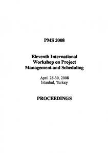
Figure 1: Different node types of a RCDG. (a), simple node, (b), conditional node, (c), merge node, and (d), supernode. associated a simple node vi ∈ VS . To each equation as defined in Def. 3.4 there are associated two special nodes: (i), one conditional node vCi ∈ VC is associated to a run-time dependent conditional CiRT to determine which of the variables x1i , x0i is selected in (ii), a merge node vMi ∈ VMi . Since, by definition the nodes vi1 , vi0 are only intermediate nodes, they can grouped together with node vi and the corresponding merge node vMi to one supernode. In Fig. 1 (a)-(d), graphical symbols of the different node types are shown. Furthermore, a set of edges E consists of two disjoint subsets E = ED ∪ EC . There is an edge (vi , vj ) ∈ ED with distance vector dij if the variable xj directly depends on xi via the dependence vector dij . Each conditional node vC RT ∈ VC coni trols one or more merge nodes vMi ∈ VMi . These control dependencies are specified by an edge (vCi , vMi ) ∈ EC . In the following small example all the definitions are wrapped-up. In the majority of cases, starting point is a given program in a high-level language like C or Java. Example 3.3 Consider the following fictive program fragment given in a pseudo language: 1 2 3 4 5 6 7 8 9

FORALL (i = 1; i ≤ N ; i + +) FORALL (j = 1; j ≤ M ; j + +) b[i, j] = b[i, j − 1]; a[i, j] = a[i − 1, j] + b[i, j]; IF (a[i, j] > 10) a[i, j] = 10; ENDIF ENDFOR ENDFOR

This program can be formulated as a DPRA as follows: b[i, j] = b[i, j − 1] a1 [i, j] = a2 [i − 1, j] + b[i, j] ( a12 [i, j] if (a1 [i, j] > 10) a2 [i, j] = a02 [i, j] if (a1 [i, j] ≤ 10) a12 [i, j] = 10 a02 [i, j] = a1 [i, j] with the iteration space I = {i, j ∈ Z | 1 ≤ i ≤ N ∧ 1 ≤ j ≤ M } common to all equations.

7

0 1

b

0 0

a1 0 0

0 0

C 1 0

a12

M

a02

a2

Figure 2: RCDG of the algorithm of Ex. 3.3. Note that in order to satisfy the single assignment property, variables have been renamed, this can be performed during a data dependence analysis of a given algorithm similar as in [Kie00] assuming that a variable defined in an if-branch have to be defined also in a corresponding elsebranch. A corresponding reduced dependence graph is depicted in Fig. 2. Here, for each left hand side variable (b, a1 , a2 ) of the DPRA exists one node. The evaluation of the run-time dependent conditional is denoted by the triangular-shaped node C which generates a control signal (dashed edge). This control signal selects in the second triangular-shaped node M whether the first or the second branch is assigned to variable a2 .

4

Allocation and Scheduling of DPRAs

Linear transformations as in the following equation are used as space-time mappings [Mol83, Len93] in order to assign a processor index p ∈ Zn−1 (space) and a sequencing index t ∈ Z (time) to index vectors I ∈ I. ! ! p Q = TI = I (2) t λ In Eq. (2), Q ∈ Z(n−1)×n and λ ∈ Z1×n . The main reasons for using linear allocation and scheduling functions is that the data flow between processor elements (PE) is local and regular which is essential for VLSI implementations. The interpretation of such a linear transformation is as follows: The set of operations defined at index points λ · I = const. are scheduled at the same time step. The index space of allocated processing elements (processor space) is denoted by Q and is given by the set Q = {p | p = Q · I ∧ I ∈ I}. This set can also be obtained by choosing

8

a projection of the dependence graph along a vector u ∈ Zn , i.e. any coprime1 vector u satisfying Q · u = 0 [Kuh80] describes the processor allocation equivalently. Allocation and scheduling must satisfy that no data dependencies in the DG are violated. This is ensured by the well-known causality constraint, λ · dij ≥ 0 ∀(vi , vj ) ∈ E.

(3)

A sufficient condition for guaranteeing that no two or more index points are assigned to a processing element at the same time step is given by ! Q rank = n. (4) λ Using the projection vector u satisfying Q·u = 0, this condition is equivalent to λ·u 6= 0 [Rao85]. If T is considered to be not anymore square, then among other things also multi-projections or partitioning schemes like Local Sequential Global Parallel (LSGP) partitioning, Local parallel global sequential (LPGS) partitioning, or co-partitioning [EM99] can be considered by an appropriate decomposition of Q and λ into sub-allocations and sub-schedules, respectively. The description of these methods would exceed the content of this report and would not result in any new insights since the following methods can similarly be applied to them. In the following we mainly focus on resource constraints in order to derive in practice applicable schedules. Definition 4.1 (Resourcegraph). A resourcegraph GR = (VR , ER ) is a bipartite graph. The set of nodes VR = V ∪ VT contains the node set V of the RCDG G = (V, E, D). Each node rr ∈ VT denotes one resource type (e.g., adder, comparator, multiplexer, etc.). An edge (vi , rk ) ∈ ER with vi ∈ V and rk ∈ VT models the possibility that vi might be executed on one instance of resource type rk . In case of a supernode only the intermediate nodes vi1 , vi0 , and the node vMi have mapping edges to resource nodes but not the node vi . Furthermore, there exists a weight function w : ER 7→ Z+ 0 which associates to each edge (vi , rk ) ∈ ER a time w(vi , rk ), the execution time of vi on rk . Let (G = (V, E, D), GR = (VR , ER )) be a given specification. An allocation of functional units is a function α : VT 7→ Z+ 0 which associates to each resource type rk ∈ VT a number α(rk ) of available instances. Furthermore, let δ(rk ) be a pipeline rate which denotes after how many time steps already a new operation can start on rk . With this resource model, let wC be the execution time to evaluate a run-time dependent conditional. Furthermore, let wF 1 and wF 0 be the execution times of the if- and the else-branch of an equation, respectively, and wmax = max{wC , wF 1 , wF 0 }. Then with respect to scheduling, different cases can be considered: 1

A vector x is said to be coprime if the absolute value of the greatest value of the greatest common divisor of its elements is one.

9

1. Static parallel branch execution. The conditional branches are (nearly) balanced if the following condition holds: wC = wmax ∨ wF 1 = wF 0 . Then, preconditioned enough resources are available, different branches of a run-time dependent conditional may be executed in parallel to achieve highest performance. These types of run-time conditionals are very common in image processing algorithms where often absolute, threshold, or min/max values are computed. Due to the balanced behavior of branches’ execution time an optimal static linear schedule can be derived at compile-time [HT04]. 2. Static mutually exclusive scheduling. If the computation of one branch is more hardware costly, it makes sense to share the resources since different branches of a conditional are mutually exclusive. 3. Branch Balancing. When the execution times of branches are different (unbalanced, |wF 1 − wF 0 | > 0), linear static scheduling may lead to sub-optimal execution times, since the worst case execution time is always given by the longest branch. Then, techniques such as loop shifting and compaction as in [GDGN04] can be investigated in order to balance the branches. 4. Quasi-static scheduling. If loop branches may not be balanced properly using branch balancing so that the overhead in execution time would not be tolerable, mixed scheduling concepts consisting of mixed static/dynamic schedules or quasi-static schedules where events generated at run-time from the evaluation of run-time dependent conditionals and trigger statically optimized sub-schedules. In the following we present a methodology, for the second case, to schedule DPRAs under resource constraints.

4.1

Static mutually exclusive scheduling

An entire mixed integer linear program (MILP) to derive optimal schedules is given in Appendix A. In this section we want to consider only the novel formulations in order to account mutually exclusive operations with resource constraints. If the number of available resources is limited, several operations may compete for the same resource. Then it has to be prevented that more than α(rk ) operations are being simultaneously executed by the same resource type rk ∈ VT . Here, we have to distinguish two different cases 1. Concurrent operations, we say also the operations are in AND relation, 2. If there are different execution branches in an algorithm, the operations are mutually exclusive, in XOR relation. The relationships among a set of operations can be represented as a tree where the internal nodes are of the above introduced types, XOR and AND, and the leaves are the operations [HHL90]. Let a node of the relationship tree have n sub-trees and the number of possible concurrent operations for each sub-tree be fj (rk , t), j = 1 . . . n. With this, the resource constraints can be formulated as

10

follows: fj (rk , t) ≤ α(rk )

∀ rk ∈ V T

(5)

∀t:0≤t≤P −1 where, fj (rk , t) is defined as follows2,3  n X   fj (rk , t)     j=1    n   max fj (rk , t) j=1 fj (rk , t) = δ(rk )−1  X   X  xi,k,t−d−νP     d=0 ∀ν:l ≤t−d−νP ≤h  i i   0

if the node is an AND node if the node is an XOR node if the node is a leaf vi ∧ ∃ (vi , rk ) ∈ ER if the node is a leaf vi ∧ @ (vi , rk ) ∈ ER

The constraint in Eq. (5) has to be generated for all different resource types and for all minus one time steps in the iteration interval. If one leaf node vi with binding possibility to resource node rk is reached, a sum of binary variables is generated. Here, by the outer summation the pipeline rate of resource type rk is considered. During the time steps from 0 to δ(rk )−1 only one operation can be executed on one instance of resource type rk . Since an operation is executed repeatedly, i.e., with a distance of P time instances, operations in different iterations may overlap and multiplies of the iteration interval (νP ) have to be considered. This is ensured by the innermost summation where the condition li ≤ t − d − νP ≤ hi can be interpreted as a convolution of the scheduling intervals to the basic iteration interval. li and hi are lower and upper bounds of t, for further details see Appendix A. In a linear program the above inequalities can be formulated only for a fixed iteration interval P (for Def., see Footnote 4) but as can seen in Appendix A, P is a variable of the MILP. This problem can be solved by the introduction of an upper bound Pmax and the introduction of further binary variables for all possible values of P . We omit this procedure for the sake of brevity.

4.2

Example

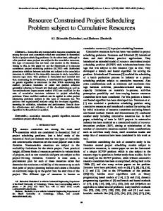
In this section, the proposed MILP formulation that can be used to schedule dynamic piecewise regular algorithms under resource constraints and to allocate necessary resources simultaneously is applied to an illustrative example. For this, consider the fictive nested loop program given in Fig. 3 (a). In this small program two nested run-time conditionals are present. An equivalent DPRA of the algorithm is represented in Fig. 3 (b). In order to formulate the scheduling problem as a MILP we have to denote the available resources. Therefore, in Fig. 4 (a) the RCDG of the algorithm and in Fig. 4 (b) a resource graph is 2

xi,k,t is a binary variable of the MILP denoting, if true, that the execution of operation vi on resource type rk is started at time t. For further details of the MILP see Appendix A. 3 A term b = max (a1 , ..., an ) can be calculated in a minimization problem by n inequalities b ≥ ai , i = 1 . . . n and the addition of b to the objective function, f (x) + b.

11

(a)

(b) a[i, j]

1 FORALL (i = 1; i ≤ N ; i + +) 2

b[i, j] = b[i, j − 1] − c[i − 1, j];

4

a[i, j] = a[i − 1, j] + b[i, j];

5

IF (a[i, j] > 10)

6

c[i, j] = b[i, j] · b[i, j];

7

IF (b[i, j] > 8)

8

d[i, j] = b[i, j] + a[i, j];

9

e[i, j] = a[i, j] + 10;

10

= b[i, j − 1] − c[i − 1, j] ( c1 [i, j] if C1 [i, j] c[i, j] = c0 [i, j] if ¬C1 [i, j] b[i, j]

FORALL (j = 1; j ≤ M ; j + +)

3

c1 [i, j]

d[i, j] = 2 · b[i, j];

12

e[i, j] = a[i, j] + 3;

= b[i, j] · b[i, j]

0

c [i, j]

= a[i, j] + 8 ( d1 [i, j] d[i, j] = d0 [i, j] ( d1.1 [i, j] d1 [i, j] = d1.0 [i, j]

if C1 [i, j] if ¬C1 [i, j] if C2 [i, j] if ¬C2 [i, j]

d0 [i, j] = b[i, j] + 3

ELSE

11

= a[i − 1, j] + b[i, j]

d1.1 [i, j] = b[i, j] + a[i, j] d1.0 [i, j]

15

c[i, j] = a[i, j] + 8;

= 2 · b[i, j] ( e1 [i, j] if C1 [i, j] e[i, j] = e0 [i, j] if ¬C1 [i, j] ( e1.1 [i, j] if C2 [i, j] e1 [i, j] = e1.0 [i, j] if ¬C2 [i, j]

16

d[i, j] = b[i, j] + 3;

e0 [i, j]

13 14

17

ENDIF ELSE

18

ENDIF

19

ENDFOR

[i, j] = a[i, j] + 10

1.0

[i, j]

e

e[i, j] = 2 · a[i, j];

= 2 · a[i, j]

1.1

e

C1 [i, j]

= a[i, j] + 3 = (a[i, j] > 10)

C2 [i, j] = (b[i, j] > 8)

20 ENDFOR

if C1 [i, j]

with I = {i, j ∈ Z | 1 ≤ i ≤ N ∧ 1 ≤ j ≤ M }

Figure 3: In (a), pseudo code of a nested loop program, in (b), the same algorithm written as a DPRA.

12

shown. Here, the available resources consist of one subtracter (sub), one adder (add), two comparators (cmp), and one multiplier (mul). Thus, six add operations and three mul operations have to share each only one functional unit. The possibility of module selection can be seen for node b which can be mapped either on resource type sub or on resource type add. All resources require one clock cycle except the multiplier which requires two cycles, but due to pipelining also the multiplier is able to start every δ(mul) = 1 clock cycle a new operation. Note, we assume that the multiplexers M1 to M5 have zero time overhead, hence binding possibilities and multiplexer resources are not depicted in the resource graph. The relationship tree of the program is shown in Fig. 5 (a), accordingly to the nesting level of the if-conditionals the tree has levels. With this information and a given allocation by a projection vector u = (1 0)T the minimization problem can be formulated. As a valid and optimal solution we obtain as schedule vector λ = (5 1), as iteration interval P = 5, and τ (C1 ) = 2, τ (C2 ) = 3, τ (b) = 0, τ (a) = 1, τ (c1 ) = 3, τ (c0 ) = 3, τ (d0 ) = 4, τ (e0 ) = 3, τ (d1.1 ) = 5, τ (e1.1 ) = 4, τ (d1.0 ) = 4, τ (e1.0 ) = 4 are the relative start times for each operation. In Fig. 6 the schedule is visualized for two processor elements for a time of each three periods. Only some data dependencies are shown. For processor element one, from left to right, three different schedules for the cases C1 [i, j] = true ∧ C2 [i, j] = true, C1 [i, j] = true ∧ C2 [i, j] = f alse, and C1 [i, j] = f alse are shown. Furthermore, it can be seen that the execution of different iterations overlap within the iteration interval P . In terms of power awareness the schedule is conscious but in terms of resource utilization, the adder and multiplier are working only 50% of the time. Therefore, it can be considered to use the free resources in order to achieve a better performance. Here, the main idea is to precompute some variables in advance before the run-time conditional is evaluated. This strategy, called speculative execution is well known and used in super-scalar and VLIW processors [SBV98]. This method will be formulated in the next section for the first time in the realm of processor array design.

4.3

Speculative Scheduling

In order to achieve highest performance, free resources can be used to precalculate speculative some variables. The main ideas to formulate the speculative execution of operations within our MILP can be summarized as follows: • Let τ (CiRT ) be the fixed execution start times of the run-time dependent conditionals. • Then, for each run-time dependent conditional two cases can be considered: 1. t < τ (CiRT ) + wC RT : The conditional has not been yet computed. Thus all of its i depending nodes are in AND relation. 2. t ≥ τ (CiRT ) + wC RT : The conditional has been evaluated and thus its branches are in i XOR relation in the following time.

13

(a)

0 1

b a

1 0 1 0

C1 C2

c1

M3

c0 d1.1 M d1.0

cc

e 1.1 M e 1.0

1

d

1

M4

2

d

e

0

1

M5

d

(b)

e0

e

1 0 1

sub

b

α(sub)=1 δ(sub)=1

1

a

1 0

1 add

1

1 0

C1

1

1

1

C2

c

1

M3

cc

α(add)=1 δ(add)=1

1

c

1 1

0

d1.1 M d1.0 d1

M4

d

α(cmp)=2 δ(cmp)=1

e 1.1 M e 1.0

1

2

d0

e1

M5

e

cmp

e0

2 2

2

mul α(mul)=1 δ(mul)=1

Figure 4: The RCDG of the algorithm in Fig. 3 (b) is shown in (a) and a corresponding resource graph in (b), respectively.

14

(a) AND

aa

b

XOR

C1 1

0

AND

cc1’

AND

cc0’’

XOR

C2 1

e0’’’

0

AND

dd1.1’

d0’’’

AND

ee1.1’

dd1.0’

ee1.0’

(b) AND

b

aa

XOR

C1 1

0

AND

cc1’

C2

XOR

’ dd1.1

AND

’ ee1.1

’ dd1.0

’ ee1.0

cc0’’

d0’’’

e0’’’

’ ee1.1

’ dd1.0

’ ee1.0

cc0’’

(c) AND

b

aa

C1

cc1’

C2

’ dd1.1

d0’’’

e 0’’’

Figure 5: In (a), relationship tree of the algorithm in Fig. 3. In (b) and (c), relationship trees in dependence on time intervals in order to perform speculation. • Furthermore, if multi-cycle operations are allowed it must be ensured that the operations’ execution can be interrupted by others. For the before discussed algorithm in Fig. 3 we get three intervals: t < τ (C1 ) + wC1

(6)

τ (C1 ) + wC1 ≤ t < τ (C2 ) + wC2

(7)

τ (C2 ) + wC2 ≤ t

(8)

In the last interval (Eq. (8)) all run-time dependent conditionals have been evaluated such that this case is equivalent to the relationship tree in Fig. 5 (a). The first (Eq. (6)) and the second (Eq. (7)) interval are depicted in Fig. 5 (c) and (b), respectively. Formulating the MILP with these relationship trees, leads to the optimized schedule shown in Fig. 7 with the schedule vector

15

C2

CMP2

C2

C1

CMP1

C1

b

PE2 SUB

c

d

1

a

ADD

b c

1.0

e 1.0

e 1.1 d1.1 a

C1

b c

1

b c

1

a

ADD

d

1

e 1.1 d1.1 a 2

P

3

e 1.0

C1

b

MUL

d1.0

C2

C1

CMP1

c1

1

a

C2

CMP2

0

C1

b

MUL

PE1 SUB

C2

4

5

6

e0

1.0

e 1.0 7

8

9

10

a 11

c0 12

13

d0 14

15

16

t

Figure 6: Gantt chart for a part of the schedule. Depicted are two processor elements for a time of each three periods. λ = (4 1), as iteration interval P = 4, and τ (C1 ) = 2, τ (C2 ) = 3, τ (b) = 0, τ (a) = 1, τ (c1 ) = 1, τ (c0 ) = 2, τ (d0 ) = 3, τ (e0 ) = 3, τ (d1.1 ) = 3, τ (e1.1 ) = 4, τ (d1.0 ) = 2, τ (e1.0 ) = 4. For instance, variables c1 and c0 are calculated speculative, in advance and in parallel to C1 . After the comparison, also c1 and c0 have been already computed, one variable is selected for the further dataflow and the other is disallowed (striped bar in the Gantt chart).

5

Conclusions and Future Directions

In this report we presented an extension of the class of PRAs in order to model run-time dependent conditionals. This extension significantly increases the range of applications which can be parallelized and mapped to massively parallel processor arrays. For instance, a lot of computational intensive applications for video and image processing consist of nested loop programs with only few and small run-time dependent conditionals. Furthermore, we presented an exact scheduling methodology which takes resource constraints and mutual exclusive execution paths into account. Finally, we presented novel extensions when designing processor arrays to utilize not used resources in order to perform speculative computations to achieve better execution performance. In the future we would like to investigate unbalanced and computational intensive branches. Here, a two-stage scheduling methodology might be applied: within a branch, a static linear schedule can be determined during compile-time. Around these static parts, a dynamic or data flow driven concept has to be developed. In case of reconfiguration at run-time our resource graph has to be extended to allow the modeling of reconfiguration times in order to perform precise worst/best case execution estimations. The newly class of DPLA introduced in this report is currently integrated into the PARO design

16

C2

CMP2

C2

C1

CMP1

C1

b

PE2 SUB

c

ADD

a

1

b

d

c

c0

d1.1 e 1.0 a

1.0

1

c1

c0

d1.1 e 1.1 a

C1

b

MUL

c

ADD

a 1

d

2

P

c

d

1

d1.1 e 1.1 a 3

d1.1 e 1.0

b

1.0

c0

c0

C1

b 1

d1.0

C2

C1

CMP1

d

1.0

C2

CMP2

0

C1

b

MUL

PE1 SUB

C2

4

5

c1

1.0

c0 6

d1.0 e 0

d1.1 e 1.0 a 7

8

9

c0 10

d0 11

12

13

14

15

16

t

Figure 7: Gantt chart for a part of the speculative schedule. system [PAR, BT01]. Furthermore, in the future we would like to adapt our design methodology in order to target also coarse-grained reconfigurable architectures [HDT04].

References [AR94]

Rumen Andonov and Sanjay Rajopadhye. An Optimal Algo-Tech-Cuit for the Knapsack Problem. Technical Report PI-791, IRISA, Campus de Beaulieu, Rennes, France, January 1994.

[BT01]

Marcus Bednara and J¨urgen Teich. Synthesis of FPGA Implementations from Loop Algorithms. In First International Conference on Engineering of Reconfigurable Systems and Algorithms (ERSA’01), pages 1–7, Las Vegas, NV, June 2001.

[BT03]

Marcus Bednara and J¨urgen Teich. Automatic Synthesis of FPGA Processor Arrays from Loop Algorithms. The Journal of Supercomputing, 26(2):149–165, 2003.

[CBF95]

Jean-Franc¸ois Collard, Denis Barthou, and Paul Feautrier. Fuzzy Array Dataflow Analysis. In Proceedings of the fifth ACM SIGPLAN Symposium on Principles and Practice of Parallel Programming, pages 92–101. ACM Press, 1995.

[CEL]

CELOXICA, Handel-C. www.celoxica.com.

[DR92]

A. Darte and Y. Robert. Scheduling uniform loop nests. Technical Report 92–10, ENSL Lyon, France, 1992.

[EM99]

Uwe Eckhardt and Renate Merker. Hierarchical Algorithm Partitioning at System

17

Level for an Improved Utilization of Memory Structures. IEEE Transactions on Computer-Aided Design of Integrated Circuits and Systems, 18(1):14–24, 1999. [Fea96]

Paul Feautrier. Automatic Parallelization in the Polytope Model. Technical Report 8, Laboratoire PRiSM, Universit´e des Versailles St-Quentin en Yvelines, 45, avenue des ´ Etats-Unis, F-78035 Versailles Cedex, June 1996.

[GDGN03] S. Gupta, N. D. Dutt, R. K. Gupta, and A. Nicolau. SPARK: A High-Level Synthesis Framework for Applying Parallelizing Compiler Transformations. In Proceedings of the International Conference on VLSI Design, January 2003. [GDGN04] Sumit Gupta, Nikil Dutt, Rajesh Gupta, and Alexandru Nicolau. Loop Shifting and Compaction for the High-Level Synthesis of Designs with Complex Control Flow. In Georges Gielen and Joan Figueras, editors, Proceedings of Design, Automation and Test in Europe, pages 114–119, Paris, France, February 2004. IEEE Computer Society. [GL96]

Martin Griebl and Christian Lengauer. The Loop Parallelizer LooPo. In Michael Gerndt, editor, Proc. Sixth Workshop on Compilers for Parallel Computers, volume 21 of Konferenzen des Forschungszentrums J¨ulich, pages 311–320. Forschungszentrum J¨ulich, 1996.

[HDT04]

Frank Hannig, Hritam Dutta, and J¨urgen Teich. Regular Mapping for Coarse-grained Reconfigurable Architectures. In Proceedings of the 2004 IEEE International Conference on Acoustics, Speech, and Signal Pro cessing (ICASSP 2004), volume V, pages 57–60, Montr´eal, Quebec, Canada, May 2004. IEEE Signal Processing Society.

[HHL90]

Cheng-Tsung Hwang, Yu-Chin Hsu, and Youn-Long Lin. Optimum and Heuristic Data Path Scheduling under Resource Constraints. In Conference proceedings on 27th ACM/IEEE design automation conference, pages 65–70. ACM Press, 1990.

[HT01]

Frank Hannig and J¨urgen Teich. Design Space Exploration for Massively Parallel Processor Arrays. In Victor Malyshkin, editor, Parallel Computing Technologies, 6th International Conference, PaCT 2001, Proceedings, volume 2127 of Lecture Notes in Computer Science (LNCS), pages 51–65, Novosibirsk, Russia, September 2001. Springer.

[HT04]

Frank Hannig and J¨urgen Teich. Dynamic Piecewise Linear/Regular Algorithms. In Proceedings of the Fourth International Conference on Parallel Computing in Electrical Engineering (PARELEC 2004), Dresden, Germany, September 2004.

[KAS+ 02] Vinod Kathail, Shail Aditya, Robert Schreiber, B. Ramakrishna Rau, Darren C. Cronquist, and Mukund Sivaraman. PICO: Automatically Designing Custom Computers. Computer, 35(9):39–47, 2002.

18

[Kie00]

Bart Kienhuis. MatParser: An Array Dataflow Analysis Compiler. Technical Report UCB/ERL M00/9, University of California, Berkeley, CA-94720, U.S.A., February 2000.

[KMW67] Richard M. Karp, Raymond E. Miller, and Shmuel Winograd. The Organization of Computations for Uniform Recurrence Equations. Journal of the Association for Computing Machinery, 14(3):563–590, 1967. [KRD00]

Bart Kienhuis, Edwin Rijpkema, and Ed F. Deprettere. Compaan: Deriving Process Networks from Matlab for Embedded Signal Processing Architectures. In Proceedings of the 8th International Workshop on Hardware/Software Co-Design, pages 13– 17. ACM Press, 2000.

[Kuh80]

Robert H. Kuhn. Transforming Algorithms for Single-Stage and VLSI Architectures. In Workshop on Interconnection Networks for Parallel and Distributed Processing, pages 11–19, West Layfaette, IN, April 1980.

[Len93]

Christian Lengauer. Loop Parallelization in the Polytope Model. In Eike Best, editor, CONCUR’93, Lecture Notes in Computer Science 715, pages 398–416. SpringerVerlag, 1993.

[Meg93]

Graham M. Megson. Mapping a Class of Run-Time Dependencies onto Regular Arrays. In Proceedings 7th International Parallel Processing Symposium, pages 97– 104, Newport Beach, CA, April 1993. IEEE Computer Society Press.

[Mol83]

Dan I. Moldovan. On the Design of Algorithms for VLSI Systolic Arrays. In Proceedings of the IEEE, volume 71, pages 113–120, January 1983.

[PAR]

PARO Design System Project. erlangen.de/research/paro.

[Rao85]

S. K. Rao. Regular Iterative Algorithms and their Implementations on Processor Arrays. PhD thesis, Stanford University, 1985.

www12.informatik.uni-

[SAR+ 00] Robert Schreiber, Shail Aditya, B. Ramakrishna Rau, Vinod Kathail, Scott Mahlke, Santosh Abraham, and Greg Snider. High-Level Synthesis of Nonprogrammable Hardware Accelerators. Technical Report HPL-2000-31, Hewlett-Packard Laboratories, Palo Alto, May 2000. [SBV98]

Gurindar S. Sohi, Scott E. Breach, and T. N. Vijaykumar. Multiscalar Processors. In 25 Years of the International Symposia on Computer Architecture (selected papers), pages 521–532. ACM Press, 1998.

19

[Sch86]

Alexander Schrijver. Theory of Linear and Integer Programming. Whily – Interscience series in discrete mathematics. John Wiley & Sons, Chichester, New York, 1986.

[SD03]

Todor Stefanov and Ed F. Deprettere. Deriving Process Networks from Weakly Dynamic Applications in System-Level Design. In Proceedings of the 1st IEEE/ACM/IFIP International Conference on Hardware/Software Codesign & System synthesis (CODES+ISSS’03), pages 90–96. ACM Press, 2003.

[Syn]

Synfora, Inc. www.synfora.com.

[Tei93]

J¨urgen Teich. A Compiler for Application-Specific Processor Arrays. PhD thesis, Institut f¨ur Mikroelektronik, Universit¨at des Saarlandes, Saarbr¨ucken, Deutschland, 1993.

[Thi92]

Lothar Thiele. Computer Systems and Software Engineering: State-of-the-Art, chapter 4, Compiler Techniques for Massive Parallel Architectures, pages 101–151. Kluwer Academic Publishers, Boston, U.S.A., 1992.

[Thi95]

Lothar Thiele. Resource Constrained Scheduling of Uniform Algorithms. Journal of VLSI Signal Processing, 10:295–310, 1995.

[TTZ97]

J¨urgen Teich, Lothar Thiele, and Li Zhang. Scheduling of Partitioned Regular Algorithms on Processor Arrays with Constrained Resources. Journal of VLSI Signal Processing, 17(1):5–20, September 1997.

[WS94]

Doran Wilde and Oumarou Si´e. Regular Array Synthesis using Alpha. In Int. Conf. on Application Specific Array Processors, San Francsico, California, pages 200–211, August 1994.

A

MILP Formulation

In this section the construction of a MILP is described. Its solution yields a latency optimal schedule and resource type binding of operations. This methodology mainly recapitulates previous ideas reported in [Thi95, TTZ97, HT01]. As is typical for VLSI processor array design, a linear schedule is applied to the DPRA with the index space I. The calculation of a variable (or an operation) xi [I] for I ∈ I starts at time step t(I) = λ · I + τ (vi )

(9)

t(I) = λ · I + τ (vi ) + wi ,

(10)

and is finished at

respectively.

20

A.1

Objective Function

The goal of the optimization is to minimize the total evaluation time L which is given by:     L = max λ · I + max {τ (vi ) + wi } − min λ · I + min {τ (vi )} vi ∈V

I∈I

I∈I

vi ∈V

(11)

In the following, L is approximated by λ · (I2 − I1 )

max

A · I1 ≥ b

subject to

A · I2 ≥ b Using the duality theorem of linear programming [Sch86, DR92] the problem can be rewritten as: min subject to

−(y1 + y2 ) · b y1 ≥ 0 , y1 ∈ Q1×m

y1 · A = λ y2 · A = −λ

y2 ≥ 0 , y2 ∈ Q1×m

λ ∈ Z1×n

A.2

Dependence Constraints

The implied data dependencies given in the RCDG have to be guaranteed. I.e., for all edges (vi , vj ) ∈ E, the computation of node vj can not begin until the execution of node vi is finished. Therefore, the starting time of vj must be at least wi greater than the starting time of node vi . The corresponding constraint tj (I) − ti (I − dij ) ≥ wi ∀ (vi , vj ) ∈ E directly leads with Eq. (9) to λ · dij + τ (vj ) − τ (vi ) ≥ wi

A.3

Determination of the Iteration Interval

The iteration interval4 is given by P = |λ · u|. Since the iteration interval is not a fixed parameter it has to be considered as variable P in the linear program. Let Pmax be an upper bound of the iteration interval, then the absolute value |λ · u| can be determined by the following set of inequalities: 4

The iteration interval P of an allocated and scheduled piecewise regular algorithm is the number of time instances between the evaluation of two successive instances of a variable within one processing element [Thi95].

21

P

≤ Pmax

λ · u ≥ P − 2vPmax

P ∈Z v ∈ {0, 1}

λ·u ≤ P

(12)

−λ · u ≥ P − 2(1 − v)Pmax −λ · u ≤ P It can easily demonstrated that the binary variable v always takes the right value so that a positive value follows, i.e., the absolute value of P .

A.4

Resource Constraints

In order to take into account resource constraints within a processing element, an additional representation is introduced. Where, the main concepts can be summarized as follows: • The scheduling of operation vi ∈ V is characterized by a binary variable xi,k,t , where xi,k,t = 1 denotes that at relative time instance t ∈ Z the operation vi starts its operation on resource type rk ∈ VT . • The relative start time τ (vi ) of each operation in the RCDG has a lower and upper bound. These bounds can be obtained from schedules following the well known as soon as possible (ASAP) and as late as possible (ALAP) principles, respectively. For this, within the processor elements unlimited resources are assumed. Through this, for each operation vi ∈ V an interval of possible starting times is determined, τ (vi ) ∈ [li , hi ], where li denotes the earliest and hi the latest possible starting time, respectively. • The relative start times τ (vi ) in Eq. (9) are represented as the weighted sum of the binary variables xi,k,t hi X X τ (vi ) = t xi,k,t ∀ vi ∈ V ∀k:(vi ,rk )∈ER t=li

• As each operation can be executed on one resource type only, we need to add the following equalities hi X X xi,k,t = 1 ∀ vi ∈ V ∀k:(vi ,rk )∈ER t=li

• The evaluation time corresponding to a node vi ∈ V executed on a resource type rk ∈ VT can then be determined as hi X X wi = w(vi , rk ) xi,k,t ∀ vi ∈ V ∀k:(vi ,rk )∈ER t=li

• And finally, in order to model resource constraints of mutually exclusive operations, the constraints that have been defined in Eq. (5) are used.

22