this work is to identify the uniqueness of hierarchical service routing compared with hierarchical network routing. Mea et al. [7] extended the service orchestration ...
Resource Optimization for Web Service Composition Xia Gao, Ravi Jain, Zulfikar Ramzan, Ulas Kozat
Abstract— Service composition recently emerged as a costeffective way to quickly create new services within a network. Some research has been done to support user perceived end-toend QoS for service composition. However, not much work has been done to improve a network operator’s performance when deploying composite services. In this paper we develop a service composition architecture that optimizes the aggregate bandwidth utilization within a operator’s network; this metric is what operators care about most. A general service composition graph is proposed to model the loosely coupled interaction among service components as well as the estimated traffic that flows among them. Then an optimization problem is formalized and proved to be NP-hard, even to approximate. Next, two polynomial-time heuristic algorithms are developed together with several local search algorithms that further improve the performance of these two algorithms. Our simulations demonstrate the effectiveness of both approximation algorithms and show that they are suitable for service graphs with varying topologies.
I. I NTRODUCTION Service composition is a key enabling technology for fast and flexible service deployment. It can be iterated to progressively integrate service components of different granularity and manage the complexity of service development. Web service technologies such as WSDL [1] provide tools to unify the semantics and syntax of service definition and access. They allow service composition to be carried out at the application level and seamlessly integrated into enterprise business logic. There has been recent interest in the service composition field to guarantee Quality of Service (QoS) when distributed service components are integrated to provide one composite service. As discussed later, existing solutions only consider QoS requirements of interest to users of each service; the classic example of such a QoS metric is the delay experienced by the user. To derive the end-to-end QoS bound, orchestration models used by existing solutions in [2], [3] are the simplistic chain (service path) model and its combination (multicast tree). Their goal is to determine the appropriate application servers that form the given service chain and whose combined performance also meets the overall QoS requirements of each individual user. Furthermore, because these solutions assume that interactions between service components conforms to welldefined logic, they are mainly suitable for low-level service composition where behavior of each component is well defined. Consequently, they cannot be used for application-level service composition where service components are loosely coupled. Little work has been done so far to improve a network operator’s performance when deploying composite services. One of the QoS metrics network operators care about most is the total aggregate bandwidth utilization within its network. This metric greatly influences the efficiency with which a network operator manages its network and the number of services that can be deployed simultaneously with a given network capacity. Furthermore, according to the current trend of
service composition exhibited by BPEL [4] and similar efforts, the orchestration model to compose service components will be fairly complex. A general graph, probably cyclic in many scenarios, is required to describe complex service composition logic among service components. This can not be handled by existing solutions [2], [3], [5], [6], [7]. To this end, this paper proposes a framework that uses a generic service graph to capture loosely coupled complex service logic and optimizes the overall bandwidth usage within an operator’s network to support a large number of service users. The paper is organized as follows. Section II discusses the related work on service composition and its QoS support, which puts our work in perspective. Section III presents our proposed system of QoS support for the generic service composition model based on web service technologies. Section IV gives the formal definition of the “service mapping” problem which maps a given arbitrary service graph to a physical network and minimizes the aggregate network bandwidth usage. Section V proves the “service mapping” problem is NP-hard to even approximate and Section VI correspondingly presents two heuristic algorithms. Section VII then presents the simulation results of the proposed algorithms with different setup. Finally, section VIII gives some discussions and section IX concludes the paper with our future works. II. R ELATED W ORK There is much work related to service overlay network, service composition and QoS support. For brevity, we only cover work that is most relevant to our research. A. Existing Service Composition Related Technologies Recently, Business Process Execution Language (BPEL) [4] has been standardized; it can define the external behavior of a service as well as its internal implementation. BPEL assumes that the interfaces of the interacting web services are defined in terms of WSDL port types and interact by exchanging WSDL messages. BPEL also defines five types of structure activities, namely, sequence, switch, pick, while and flow. With these five orchestration activities, BPEL can define very complex web service composition logic. Recently, there has been work on how to manage QoS provisioning for composed services [2], [3], [5], [6], [7]. Gu [2] and Xu [5] use an application-level virtual link orchestration model that organizes service components into a chain architecture; i.e., a service path. As shown in Fig. 1, composite service logic is implemented by composing the basic service components between a service entrance portal and service exit portal. Each service component has a service level agreement (SLA) specifying availability and response time. Each link between adjacent service components is also characterized by its availability and transmission delay. The final goal of the work is to compose a service path among
2
all service components that can best avoid QoS violations or mitigate such a violation should one occur.
link is deterministic. Such an assumption is suitable for services, such as streaming, which have well-defined functional units that can be deployed at each node along the service path. But it is too restrictive for loosely coupled services such as web services.
Composite Service Service Input Portal
Fig. 1.
Service Component 1
Service Component 2
Service Component 3
Service Output Portal
Service path model of service composition.
Jin et al. [3] extend the single service path orchestration model by providing service composition functionalities to multiple users with distributed location and heterogeneous service requirements. Hence, a one-to-many multicast tree orchestration model is used. Compared with the scheme of building multiple one-to-one unicast service paths between the source and each destination node, the one-to-many multicast orchestration model can save both computing power at intermediate service nodes and bandwidth of intermediate links by combining common segments of unicast service paths. The final goal of the work is to build an optimal multicast service tree that meets bandwidth requirements and minimizes the aggregate delay and/or the total number of hops. Jin et al. [6] also proposed an distributed and hierarchical service composition architecture. In this work, the service overlay network is first organized into a cluster architecture and then the service path finding algorithm is applied hierarchically in a divide-and-conquer fashion. The main focus of this work is to identify the uniqueness of hierarchical service routing compared with hierarchical network routing. Mea et al. [7] extended the service orchestration model from a single service chain to a generic directed acyclic graph. Then sFlow, a distributed service routing algorithm, was developed to choose appropriate servers that satisfy the service logic requirement and optimize the QoS metrics. B. Limitations of Existing Solutions To motivate our work, we now describe limitations of existing solutions. 1) Existing work on QoS support in service composition aims to guarantee QoS metrics that each service user will experience (e.g., bandwidth and delay). They do not account for QoS metrics that a network operator cares about (e.g., aggregate bandwidth). Total aggregate bandwidth usage within a network influences the efficiency with which a network operator manages its network and the number of services that can be deployed simultaneously with a given network capacity. 2) To derive end-to-end QoS bounds, existing solutions [2], [3], [5], [6], except [7], use simple orchestration models such as single chains (service path) and combinations of chains (multicast tree). According to the current trend of service composition exhibited by BPEL and similar efforts, the orchestration model to compose service components will be much more complex than a chain architecture. A general graph, probably cyclic in many scenarios, is required to describe complex service composition logic among service components. This cannot be handled by existing solutions. 3) Existing work assumes a closely coupled relation between adjacent service components in the sense that the behavior at each service node and interconnecting
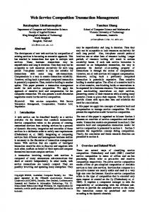
III. S ERVICE C OMPOSITION M ODEL AND S YSTEM A RCHITECTURE In previous section we have discussed the major limitations of existing service composition models. In this section we at first present a new model that is more suitable for webtechnology based service composition. We then propose a system architecture that enables a network operator to improve its network efficiency when composing distributed services. A. Generic Service Composition Model Figure 2 shows the service composition graph that a network operator uses to support the business of a travel agent. The Service Proxy/Gateway is the data entrance point of the 3rdparty service provider and its end users. All the entities shown in Figure 2 are service components that the service agent requires from the network operator. 3rd-party service provider gives its own web site and core value-added services to end users and redirects traffic to these supporting servers upon user request. For the travel reservation, users can go to Flight Reservation, Hotel Reservation, or Car Rental Reservation directly. Users can also go to a Deal Search Service to find the best available deal and then make reservations. After making the reservation, the billing is handled by Payment Processing and the Shipping Service takes care of the mailing of receipts, tickets, and other materials. To increase profit, the 3rd-party service provider has a contract with Shopping Sites and attracts users to these shopping sites to purchase travel-related merchandize such as sports gear, books, and souvenirs. To increase the user base, the 3rd-party service provider utilizes a Unified AAA Service to provide a single sign-on experience to end users. Some of the auxiliary services useful for travel arrangements are the Weather Channel and Local News. If some of the news or events are in the form of audio or video, a Media Streaming service could be used. The graph of web service composition just shown has two Weather Channel
Service Proxy / Gateway
Deal Search Service
Local News
Media Streaming
Shopping Sites
Flight Reservation
Hotel Reservation
Car Rental Reservation
Unified AAA Service
Payment Processing
Shipping Services
Fig. 2.
Service Composition Graph of a Travel Agent.
major differences compared to the service composition model described in the related work. Firstly, the topology of the web service composition graph is too complicated for existing models to readily handle. In many cases the composition model has to be expressed as a directed cyclic graph. As exemplified in Fig. 2, the proxy
3
server, news, and streaming form a circle. The Proxy server, flight reservation, Payment processing and Shipping blocks form a service chain while flight reservation, rental reservation and hotel reservation form a parallel architecture. Secondly, the functionality and QoS metric can not be accurately defined for the service nodes and service links in the graph. This is because each service component might be another service provider with very complicated service logic. For reasons such as security, most of the service logic will not be exposed and the service can only be accessed through a well-defined API. Fulfilling a service request might require multiple back and forth messages between neighboring nodes. Hence, the functionalities of each service component cannot be easily depicted (in many cases requiring run-time user input) and the QoS of each service component and accordingly the end-to-end QoS is hard to defined at setup time. As a result, the links defined in this graph are no longer the logic interaction between two nodes. Instead, it shows there is noticeable traffic flowing from the source node to destination nodes. The traffic includes all the messages of one conversation and also is the aggregate message traffic of all users using the services. B. System Architecture Figure 3 shows the basic system architecture of the service composition within an operator’s network. It includes both an operator’s network and its interacting peers outside of its trusted domain. A network operator deploys the Service Composition Engine within its trusted domain to manage the service composition process. The Service Composition Engine obtains currently available services both within and outside the networks from the Service Registry. The Service Registry stores the information of service type, characteristics, access information, and other related details and supports different kinds of queries. For example, one Service Registry technology, UDDI [8], can find registry entries that satisfy search criteria such as a particular business entity, a particular service type, access information, and semantic details contained in the model. Network management monitors the bandwidth usage of each link and computation capacity of each application servers/routers within the network. With all the information, the service composition engine calculates the optimal server assignment and sends the results to Service Configuration to configure the involved application servers. The configuration includes a service identifier to uniquely identify a composite service and the addresses of adjacent application servers to forward data traffic of users using this composite service. The service used for composition can be provided by internal application servers owned and operated by the network operator or by external application servers owned and operated by 3rd parties outside of the trusted space but accessible through well-defined interfaces. To interact with 3rd-party application server, an application proxy is used by the network operator to take care of the message transformation, asynchronous and synchronous transformation, AAA and other coordination functionalities. 3rd-party service providers offer services to end users. To build the services, the 3rd-party service provider decides which parts of the service logic will be implemented locally and what should be supported by the network operators. Before making such a decision, 3rd-party service providers might send inquiries to the Service Registry to ask for information of
3rd-party Application Servers
3rd-party Service Provider
Application Proxy
Application Proxy /Gateway
Service Composition Engine
Service Registry
Service Configuration
Network Management
End user of 3rd-party Services Application Servers
Fig. 3.
Internal Composite Services
Routers
System Topology of Service Composition.
available services within the network. With this information, 3rd-party service provider can then choose the set of service components that will be supported by the network operator. Once this decision is made, the service provider will sign a Service Level Agreement (SLA) with the network operator to decide the QoS metrics including the total number of users and total bandwidth. With this information, the 3rd-party service provider is able to produce the service composition graph and specify the traffic on each link connecting two service components. Such a service composition graph is then sent to the Service Composition Engine for the optimal deployment. After the service graph is optimally deployed, each end user accessing the composite services will be redirected to application servers within the operator’s network. Because each composite service is uniquely identified by a tag, application servers are able to distinguish user requests from different composite services and route the request to the subsequent application server. In Fig. 3, solid lines denote signaling flows during the service deployment phase and dashed lines denote data flow when end users request services. IV. S ERVICE M APPING P ROBLEM D EFINITION After presenting the framework to provide QoS support for complex service composition, we formally define the “service mapping” problem (SMP) that is studied in detail in the rest of the paper. Let service graph Gs = (Vs , Es ) be a directed graph with vertex set Vs (|Vs | = Ns ) and edge set Es (|Es | = Ne ). Each node vs ∈ Vs is a service component that is required by the 3rd-party service provider. Every edge es (vi , vj ) ∈ Es has an associated cost c(es ), which is the estimated traffic from a source node vi to a destination node vj . Let Ps = (Vp , Ep ) be a directed graph that describes the network topology of a network operator. Node set Vp consists of a set of application servers Va and intermediate routers Vr . Each service component vs ∈ Vs in the service graph is supported by a set of application servers S(vs ) in the network graph. S(vs ) is a non-empty subset of Va . For every pair of application servers in Va , a distance function, d(va,1 , va,2 ), is defined, which is the hop distance of the physical path in the network graph Ps from source node va,1 to destination node va,2 . The aggregate bandwidth utilization C(Gs , Ps , Va ) is defined according to the following formula: X c(es ) · d(f (vi ), f (vj )) (1) es (vi ,vj )∈Es
Then the goal of an optimization algorithm for SMP is to define the mapping function f : Vs 7→ Va that uniquely assigns each service component vs to an application server f (vs ) ∈
4
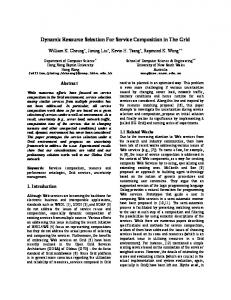
S(vs ) that supports vs while minimizing C(Gs , Ps , Va ) within the network operator’s network Ps to deploy the whole service graph Gs . In Eqn. 1, for each service link es (vi , vj ), the product of the traffic c(es ) on this link and the hop distance d(f (vi ), f (vj )) between corresponding application servers in the network graph Ps is calculated. This product captures the effect that the traffic from service component vi to vj will use the resource of multiple links in the underlying network that interconnect two supporting application servers f (vi ) and f (vj ). Figure 4 shows an example of SMP that maps a service graph to the underlying physical network and minimizes aggregate bandwidth utilization. Service Composition Graph Gs
Service Vs,2
10 Kbps 15 Kbps Service Vs,1
Service Vs,3
100 Kbps
Application servers Overlay Network Ms
S3(Vs,2)
S4(Vs,2) S5(Vs,3)
S2(Vs,1)
10*3=30 15*3=45
S1(Vs,1) Physical Network Ps
S6(Vs,3)
100 * 4 = 400
S2
S3 S5 R1
S1
R6
R2 R3
Fig. 4.
S4
R4
S6
R5
Example of service mapping problem
There are three different service components, Vs,1 , Vs,2 , and Vs,3 required from the 3rd-party service provider. The service graph formed by Vs,1 , Vs,2 , and Vs,3 is a circle. The weights of links among Vs,1 , Vs,2 , and Vs,3 show the estimated traffic flowing among them. There are six application servers in the physical network supporting these service components. Server s1 and s2 support service Vs,1 ; s3 and s4 support service Vs,2 ; s5 and s6 support service Vs,3 . These servers are distributed at different physical network locations and connected with each other through intermediate routers. For example, the link from s1 to s3 has the shortest path of length 3. Then the optimization problem is to choose an application server among s1 , s2 for Vs,1 , a server among s3 , s4 for Vs,2 , and a server s5 , s6 for Vs,3 such that the aggregate bandwidth-distance product for the chosen set of application servers is minimized. If servers s1 , s3 , and s6 are chosen, then the aggregate bandwidth-distance product for this set of servers is 475kbps. Observe that the optimal set of servers can be found by considering all possible combination of servers, but this approach has exponential time complexity. Given a generic service graph with arbitrary topology and traffic requirement and a network graph having a number of servers for each service component, it is NP-hard to compute the optimal set of servers, as we will show, and therefore unlikely to be computable in polynomial time. Of course, for specific classes of graphs, one may be able to obtain more efficient solutions. A. Integer programming formulations To develop exact algorithm for the SMP defined in Eqn. 1, we formally formulate it as an integer programming (IP)
problem so that standard linear programming and integer programming techniques can be used to find the optimal solution. In order to formulate the problem, we compose an overlay network of application servers Ms = (Vm , Em ) from the given service graph Gs and network graph Ps . The node set Vm of Ms consists of all the application servers that support a service component of Gs . So Vm is equal to Va . A link em ∈ Em is defined from node si (vi ) to sj (vj ) if and only if there is a service link es in graph Gs from service component vi to vj . For each link em from node si (vi ) to sj (vj ) we define a weight function c(em ) = c(es (vi , vj )) · d(si , sj ); i.e., the bandwidthdistance product of em . An example of composing overlay network Ms is also shown in Figure 4. Here we assume that each application server supports only one service component. Later we will describe the process to decompose a server supporting multiple service components into multiple servers supporting only one service component each. So techniques described here are still feasible. The integer programming formulation of the SMP is then based on the composed overlay network Ms . We define for each server sm (vi ), a variable ysm which is equal to one if server sm is chosen to support service component vi , and zero otherwise. We define for each em (si (vi ), sj (vj )) ∈ Em , a variable xem which is equal to one if edge em is included in the mapping, and zero otherwise. We further consider three additional constraints imposed by the service mapping problem. For each vi , only one application server is chosen from the set, S(vi ), of all servers supporting vi . So we introduce the constraint X ysm = 1, ∀vi ∈ Gs . (2) sm ∈S(vi )
Let E(i, j) be the set of all the links in Ms that point from servers supporting service vi to servers supporting service vj . Because there is only one link chosen in E(i, j) that goes from a server chosen to support vi to another server chosen to support vj , we introduce the constraint X xem = 1, ∀vi , vj ∈ Vs , vi 6= vj . (3) em ∈E(i,j)
Furthermore, if an application server sm is chosen to support a service component vi , all traffic incident to the service component vi must enter or leave the same server sm . So, all the links incident to the chosen server are included in the mapping and none of the links of other servers supporting vi are included. Let D(vi ) be the sum of the in-degree and outdegree of a service component vi in Gs and E(sm ) be the set of all links in Ms that enter or leave sm . We introduce the constraint X xem = D(vi ) · ysm , ∀sm ∈ Vm . (4) em ∈E(sm )
Combining these constraints, we obtain the ger programming formulation of the SMP: P minimize c(em )xem P em ∈Em subject to sm ∈S(vi ) ysm = 1, P xem = 1, vi 6= vj , Pem ∈E(i,j) em ∈E(sm ) xem = D(vi )ysm , xem ∈ {0, 1}, ysm ∈ {0, 1}.
following inte-
∀vi ∈ Gs ∀vi , vj ∈ Vs ∀sm ∈ Vm (5)
5
After SMP is formulated as a standard integer programming problem, techniques such as branch and bound [9] can be used to derive the optimal value. Branch and bound divides original feasible solution set into many smaller feasible solution sets and then solves subproblems on these smaller sets. During the calculation, it uses bounds on the optimal cost to avoid exploring certain subproblems. A popular method to obtain such a bound is to use the optimal cost of the linear programming relaxation. Typically techniques such as branch and bound have better performance than brute force search. However, there are O(Va2 ) variables xem and O(Va ) variables ysm in Eqn. 5. 2 So in worst case, branch and bound has to calculate O(2n ) subproblems and the time complexity is still exponential. In the following section, we will prove that the SMP is indeed NP-hard. Accordingly we will propose two approximation algorithms and prove their approximation ratio. V. NP-H ARDNESS OF S ERVICE M APPING P ROBLEM The time required to solve the SMP depends on the topologies of service graph Gs and the network graph Ps and the number of application servers for each service component. For some special cases, SMP can be solved efficiently. For example, if there is only one application server for each service component, then no matter how many service components Gs has, the total number of server combination is one and SMP is solved in constant time. Another example is the simple chain topology which can be handled in polynomial time by modifying Dijkstra’s shortest path algorithm [3]. However, a brute-force algorithm requires super polynomial time in general. For example, for a service graph with k service components and a physical network that has 3 servers for each service, the total number of server combination is 3k , which is exponential in k. In this section, we will prove the NP-hardness of SMP by reducing the well-known NP-complete problem 3-CNF-SAT to it (3-CNF-SAT was proved NP-hard by Cook [10]). We then show, the problem is hard, even to approximate, within a constant factor. The 3-CNF-SAT has following definition. A Boolean formula φ is in 3-conjunctive normal form, or 3-CNF, if φ = C1 ∧ . . . ∧ Ck , where each Ci is the disjunction of exactly three literals. A literal in the formula is an occurrence of a variable or its negation. Assume that there are n variables total; call these x1 , . . . , xn . For example, the Boolean formula φ = (x1 ∨ x2 ∨ x3 ) ∧ (x3 ∨ x2 ∨ x4 ) ∧ (¬x2 ∨ ¬x3 ∨ ¬x4 ) (6) is in 3-CNF. The 3-CNF-SAT problem is to find out whether a given Boolean formula φ is satisfiable; i.e., there is an assignment of the variables for which the formula evaluates to true. We focus on the decision version < Gs , Gp , c > of the SMP, which is described as follows: can we choose one server (among all servers in Gp ) for each service component in Gs such that the sum of bandwidth-distance product of all links among these chosen servers in Gp is at most c. The NP-hardness of the optimization version of SMP follows immediately from the NP-completeness version of the decision version. Theorem 1: The Decision Service Mapping Problem (DSMP) is NP-Complete.
Proof: It is easy to see that DSMP ∈ NP. Given a instance of decision problem < Gs , Gp , c > that has total ` = |Va | servers, it takes O(`2 ) to sum the bandwidth-distance product of all links among these servers and decide whether the sum is bounded by c. We now show NP-hardness of DSMP by reducing 3-CNFSAT to it. Given the instance of 3-CNF φ = C1 ∧. . .∧Ck with k clause, we convert it to an application overlay network Ms of SMP as follows. The graph Ms has k sets of 3 vertices. Call these sets S(v1 ), . . . , S(vk ). Each S(vi ) contains 3 vertices (corresponding to the literals in ith clause) where all 3 vertices in S(vi ) support the same service component vi . Now, we place a directed from each vertex in each S(vi ) to each vertex in S(vj ), i 6= j. The weight of the directed edge is α if two vertices of the edge do not correspond to literals that are the negation of each other and is β otherwise (e.g., the edge weight is β on the edge between vertices corresponding to x1 and ¬x1 ). Further, we pick α < β. Hence, the generated Ms has three characteristics. First, the service graph Gs is a clique. Second, the bandwidth-delay product of each link is either α or β. Third, there are exactly 3 servers supporting each service component in Gs . Now, we claim that the original formula φ is satisfiable iff the resulting SMP has an aggregate bandwidth-distance product of n(n − 1)α. First, suppose the original formula is satisfiable. Then, there is a satisfying assignment to the literals x1 , . . . , xn . For each clause, there must be one literal whose value is true within that clause. Pick one such true literal from each clause. Consider the vertices si (vi ) corresponding to the true literal in clause Ci belonging in set S(vi ) in Ms , for 1 ≤ i ≤ k. Now, this collection of vertices forms a clique (since there is an edge between every vertex in one clause and every vertex in another clause). Moreover, because in two clauses both the literals evaluate to true, they cannot be negations of each other. Therefore, each links has a bandwidthdistance product of α. We have n(n −1) edges (since we have n(n − 1)/2 pairs and there is one edge in each direction). The sum of these values is n(n − 1)α. This provides a proof for one direction. Now, let us assume that Ms has a service assignment of weight n(n − 1)α. In this case, consider the vertices in the clique. The literals corresponding to these vertices can be set to true. This gives a satisfying assignment to each clause. Moreover, we have no contradictions since the clique weight is n(n − 1)α, but the weight between any literal and its negation in another clause would be β; therefore the edge is not in the clique since its inclusion would yield a weight greater than n(n − 1)/α since β > α. Therefore, the algorithm for converting the formula to Ms constitutes a reduction. Finally, it is not hard to see that this reduction can be computed in polynomial time. This follows since the graph Ms has 3k vertices. So we can initialize the adjacency matrix in at most 9k 2 steps. Filling it is straightforward and can be done with a single scan of the formula. Thus the whole reduction is polynomial time. � The reduction is depicted in Fig. 5 using Eqn. 6 as an example. Now, let us examine what this reduction yields with respect to approximation ratios. Suppose that there is a polynomialtime algorithm that always performs within an approximation factor of ˆb. We claim that the existence of such an algorithm would imply P = N P . The reasoning is simple – if we construct the graph used in the above reduction where β is
6
Service Graph
Cmin . The aggregate bandwidth-distance product, Cappro , of any approximation algorithm’s solution is no bigger than . . C max ˆ. ≤ C Cmax . So the approximation ratio α = appro C Cmin = α �
V2
v1
1
3-CNF-SAT Reduction 1
S1(V2)
S2(V2)
S3(V2)
1 X3
V3
X2
X4
α
Fig. 5.
S1(V1)
X1
S2(V1)
X2
S3(V1)
X3
X2
β
α
β
β
β
S1(V3)
X3
S2(V3)
X4
S3(V3)
Reduction of 3-CNF-SAT in Equation 6
especially computed to be sufficiently larger than α, then the gap between the optimal solution and any suboptimal solution would be large. Therefore, any algorithm performing within a given approximation bound would necessarily pick the optimal solution. However, the optimal solution results in a satisfying assignment for the formula φ on which the graph is based. Specifically, if we set � 1 �ˆ b (n(n − 1)α) − (n2 − n − 2)α , (7) β> 2 then this is sufficient. Here’s why. The optimal algorithm would yields a solution of weight n(n−1)α. Any “suboptimal” solution must have at least one β edge (in each direction). Therefore, a suboptimal solution has weight at least (n(n−1)− 2)α + 2β. And the approximation ratio of such a suboptimal solution is: (n(n − 1) − 2)α + 2β . n(n − 1)α Now, if the above quantity is greater than ˆb, then the supposed approximation algorithm must pick the optimal solution (otherwise it failed to meet its claimed approximation ratio). Setting β according to eqn. 7 is sufficient. Therefore, we have proved: Theorem 2: For any constant ˆb, there is no polynomial-time algorithm for SMP with approximation ˆb unless P = N P . VI. A PPROXIMATION A LGORITHMS In this section, we introduce two polynomial time “heuristic” approximation algorithms that provide a feasible, but suboptimal, solutions to SMP. We also prove a generic (nonconstant factor) upper bound α ˆ on the approximation ratio of any algorithm that yields a feasible solution. We further prove that in the worse case the approximation ratio of both approximation algorithms are equal to α ˆ . Our simulations later show that both algorithm perform very well in reality. For example, in our simulation, when α ˆ is 12, both algorithm has approximation ratio less than 2 for the types of graphs encountered in practice. Given a service graph Gs , a network graph Ps , and a set of application servers Va in Ps , we form the overlay network of application server Ms . Let Ne be the number of links in Gs , Cmax be the sum of the Ne highest bandwidth-distance product of all links in Ms , and Cmin be the sum of the Ne lowest bandwidth-distance product of all links in Ms . Lemma 1: Any feasible SMP algorithm has an approximamax tion ratio of at most α ˆ=C Cmin . Proof: The optimal value, C, of SMP is bounded from below by Cmin because any feasible solution of SMP is no less than
A. Minimum-weight Heuristic Approximation Algorithm The Minimum-weight approximation algorithm (MW)discussed in this section and the longest chain approximation algorithm discussed in the following section are both greedy. They differ from each other in the order they organize and search service components in Gs . The search order of MW is based on the observation that many service graphs have a parallel fan-out architecture. One example of such a fan-out architecture is the service graph of a travel agent shown in Figure 2. Part of this figure shows traffic of the travel agent’s users flows through “service proxy/gateway” to services of “flight reservation”, “hotel reservation”, and “car rental” in parallel. And then the billing traffic from these services flow to a “payment processing” service in parallel as well. To take advantage of such an inherent fan-out architecture in many complex service graphs, MW first runs breadth-first search (BFS) in a service graph and uses the resulting BFS tree to arrange all service components. The root of the BFS tree is the service proxy/gateway with depth 0. The leaf nodes will have the largest depth. Because the purpose of BFS is to arrange service nodes according to their distance from the root, BFS uses hop distance as the metric. Then MW begins its greedy procedure from the leaf nodes to the root node in decreasing order of nodes’ depth. For each service component vi , each of its supporting servers sm (vi ) ∈ S(vi ) calculates a local weight function w(sm (vi )). The server with the lowest weight w(sm (vi )) is chosen to support service component vi . This procedure is repeated until all service components have been assigned to a server. The local weight function w(sm (vi )) is calculated as follows. At the beginning of the iteration, MW initializes the weight function w(sm ) of each server to zero. Then, for a chosen service component vi , the local weight of its supporting server is calculated using the formula: X w(sm (vi )) = c(es ) · d(sm (vi ), f (vj )). (8) vj ∈adje(vi )
In Equation 8, adje(vi ) = {vj |vj ∈ Vs , es (vi , vj ) ∈ Es } is the set of neighboring nodes of vi in Gs . We let c(es ) denote the estimated traffic on the service link es and let d(sm (vi ), f (vj )) denote the hop distance of the route from application server sm (vi ) to the application server f (vj ) supporting service component vj . If f (vj ) has not been assigned yet, the shortest distance from sm (vi ) to any server supporting vj is chosen as d(sm (vi ), f (vj )). The pseudocode of the MW is shown in Fig. 6. Fig. 7 shows an example of using the MW to solve SMP. There are 5 service components in the service graph. For each service component, there are two application servers supporting it; namely, server i and j for Vs1 , server e and f for Vs2 , server g and h for Vs3 , server c and d for Vs4 , and server a and b for Vs5 . All links between two application servers have length 2, except from e to a and from c to e, which we assume have distance 1. Fig. 7 shows the results of BFS search and local weight calculation of each application
7
Minimum-weight Algorithm( Input: Gs, Ps, Va) { Run BFS search in Gs ; Order nodes of Gs in the decreasing order of depth ; Set weight w of each server sm to 0 ; foreach ( vi in Gs ) { foreach ( sm in S(vi) ) calculate weight w(sm) ; assign sm with minimum weight to support vi ; } } Fig. 6.
1
Vs2
3
1
Vs1
2 Vs4
2
Vs5 2
Vs3 Breadth-first Search Tree Vs1
Application Server
3 ⋅ 2 + 2 ⋅ 2 = 10
Vs2
Vs5
Vs3
Vs4
3 ⋅1 = 3 e(Vs2)
3⋅ 2 = 6
i(Vs1)
f(Vs2)
j(Vs1)
2⋅2 = 4 g(Vs3)
3⋅ 2 + 2 ⋅ 2 = 10
h(Vs3) 2⋅2 = 4 Fig. 7.
0 a(Vs5) 0 b(Vs5) 1 ⋅1 + 2 ⋅ 2 = 5 c(Vs4)
d(Vs4) 1⋅ 2 + 2 ⋅ 2 = 6
Example of minimum-weight algorithm
server. The chosen application server is marked with thicker box. We break ties randomly. Since the BFS search in Gs takes O(Vs + Es ) time and the calculation of local weights of servers in Va takes at most O(|Va |2 ) time, the time complexity of MW is polynomial. The approximation ratio of MW is given in the following theorem. Theorem 3: MW has an approximation ratio of α ˆ. Proof: Lemma 1 shows that α ˆ is an upper bound for any approximation ratio. So, we only need to prove that α ˆ is reachable for MW . Consider the instance shown in Fig.8. The service graph Gs is a chain. There is one server (a) for vs1 , two servers (b and c) for vs2 , two servers (d and e) for vs3 , and one server (f ) for vs4 . The composed overlay network Ms has the link weights shown in the figure. It is easy to see that the optimal server assignment is {a, c, e, f }, which has bandwidth-distance product m. MW chooses {a, b, d, f }, which has bandwidth-distance product 3(m − 1). The approximation ratio for this scenario is α = 3(m−1) and the upper bound is α ˆ = 2m+(m−1) . As m m m−1 goes to ∞, α approaches α ˆ. � Notice that Theorem 3 provides a worst-case approximation ratio. Our simulation results later show that MW performs very
Overlay Network Ms
Vs1
a(Vs1) 0
m-1
Vs2
b(Vs2) m m-1
Vs3 Vs4 Fig. 8.
Pseudocode of Minimum-weight algorithm
Service Graph
Service Graph Gs
m c(Vs2) 0
d(Vs3)
e(Vs3)
m-1
m
f(Vs4)
The worst case of minimum weight algorithm
well in most of the scenarios. B. The longest chain heuristic approximation algorithm The previous section discussed the MW which targets service graphs with parallel fan-out architecture. In this section we present another greedy algorithm, the longest chain approximation algorithm (LC), that is geared towards service graphs with more sequential architecture. The service chain graph discussed earlier is an example of this architecture. To find the inherent sequential architecture in a complex service graph, LC first runs depth-first-search (DFS) in the service graph. Because DFS can produce several disconnected DFS trees, LC manipulates these DFS trees one at a time. For each DFS tree, the longest service path is from the root to the leaf with the largest depth. Then, the second longest chain in this DFS tree is found whose source node is on the first service chain and whose destination node is another leaf. This procedure continues until all service nodes in this DFS tree are covered by some service chain. After service chains have been found in all DFS trees, they are ordered from the longest to the shortest. Ties are broken randomly. Longest-Chain Algorithm( Input: Gs, Ps, Va) { Run DFS search in Gs ; foreach ( DFS tree) find all service chains in the tree; Order service chains SCk in the decreasing order of length ; Set weight w of each server sm to 0 ; foreach (SCk ) { form overlay network Ms(SCk) ; foreach ( sm in Ms(SCk) ) calculate weight w(sm) ; foreach (pair of root server and leaf server ) calculate the shortest path; choose the path Pi with lowest weight ; assign all sm(vi) on path Pi to support vi ; } }
Fig. 9.
Pseudocode of the longest chain algorithm
Then, beginning with the longest service chain, LC decides the mapping of service components on each service chain. For each service chain SCk , LC first composes the overlay network Ms (SCk ) of application servers using SCi as the service graph. Then each server sm uses Eqn.9 described below to calculate the local weight w(sm ). LC then runs the shortest path algorithm in Ms (SCk ) from application servers supporting root service component to application servers supporting the leaf service component. The path with the lowest weight is chosen and servers on this path are selected to support corresponding service components. Finally, LC decides whether all service chains have been calculated; if so, it terminates. The pseudocode of LC is shown in Fig. 9.
8
The local weight calculation in LC is almost the same as the calculation in MW. The only difference is that the bandwidth-distance product of the service link from a server to its immediate child in the service chain SCk is excluded from the weight calculation. This is because the bandwidth-distance product of this link has already been included in the calculation of the shortest path. Hence, the local weight calculation of LC is: X w(sm (vi )) = c(es ) · d(sm (vi ), f (vj )) (9) vj ∈adjesc (vi )
and adjesc (vi ) = {vj |vj ∈ Vs , es (vi , vj ) ∈ Es , es (vi , vj ) ∈ / SCk }. The weight of a path of service chain SCk is calculated as follows: X X c(es ) · d(f (vi ), f (vj )) + w(f (vi )).
Service Graph Gs Vs1
(10) Fig. 10 shows an example of using LC to solve SMP. Gs , Ps , and Va are the same as those in Fig.7. The DFS produces one DFS tree. In this tree, the longest chain is Vs1 → Vs2 → Vs3 of length 3. The second chain is Vs1 → Vs3 → Vs4 . Since the root of the second chain is already included in the first chain, the length of the second chain is 2. The weight calculation of each application server is shown in the example. Also shown is the calculation of shortest path according to Eqn. 10. After application servers on the first service chain are chosen, the application servers on the second service chain are chosen in the same way. The chosen application servers are denoted with a solid box. Service Graph
3
Vs2
3
1
Vs1
2 Vs4
2
Vs5 2
Vs3 Vs1
Depth-first Search Tree
Vs2 Vs3
Overlay Network Ms i(Vs1) 0 j(Vs1) 0 4 4
3⋅ 2 = 6 6 6 6
Vs5 Vs4
0 3 ⋅1 = 3 0 e(Vs2) a(Vs5) 6 0 0 f(Vs2) 6 b(Vs5) 6
0 2 ⋅ 2 = 4 2 ⋅1 + 2 ⋅ 2 = 6 g(Vs3) 4 c(Vs4) 4 h(Vs3) 4 d(Vs4) 0 2⋅2 + 2⋅2 = 8
Example of the ”longest service chain” approximation problem
LC runs in polynomial time since each step of LC finishes in polynomial time.The computation of LC is much more complex than MW. However, its time complexity is greater than that of MW. In the following, we prove the approximation ratio of LC, however, is the same as MW in the worst case. Theorem 4: LC has approximation ratio α ˆ. Proof: Lemma 1 has shown that α ˆ is the upper bound for any approximation ratio. So, we only need to prove that α ˆ is reachable for LC.
Overlay Network Ms
Vs2
Vs4
Vs3
Vs5
m
a(Vs1) m-1
b(Vs2) m-1
vi ∈SCk
es (vi ,vj )∈SCk
Fig. 10.
Consider the instance shown in Fig.11. Running DFS in Gs produces two chains, Vs1 → Vs2 → Vs3 and Vs1 → Vs4 → Vs5 . There is one server (a) for vs1 , two servers (b and c) for vs2 , two servers (d and e) for vs3 , one server (f ) for vs4 , and one server (g) for vs5 . The composed overlay network Ms has the link weights shown in the figure. It is easy to check that optimal server assignment is {a, c, e, f, g}, which has bandwidth-distance product 4m. LC chooses {a, b, d, f, g}, which has bandwidth-distance product 6m − 2. The approxand the upper imation ratio for this scenario is α = 6m−2 4m 6m bound is α ˆ = 4m−2 . As m goes to ∞, α approaches α ˆ. �
m m m
m c(Vs2)
0
f(Vs4) m
m m
d(Vs3)
g(Vs5)
0
e(Vs3) Fig. 11.
The worst case of the longest chain algorithm
C. Local search algorithms In this section, we will present several local search algorithms that further improve the performance of MW and LC. The main idea of these local search algorithms is to start at the assignment f (Gs ) produced by MW and LC, and then evaluate the aggregate bandwidth-distance product C for some other assignment f 0 (Gs ), which is a “neighbor” of f (Gs ). If a neighbor f 0 (Gs ) with lower C is found, select f 0 (Gs ) and repeat the same process. If no such neighbor is found, the process stops: a local optimum has been found. There is a generic tradeoff in such local search algorithms. When we consider larger neighborhoods, there are few local minima and a better solution is likely to be found when the algorithm terminates. On the other hand, the algorithm is slower since more feasible solutions have to be compared. The three local search algorithms presented here follow the same logic and only differ in the way they define “neighborhood”. 1OPT local search considers assignments f (Gs ) and f 0 (Gs ) neighbors if we can obtain one from the other by changing the assignment of one service component. Similarly, 2OPT and 3OPT local search considers f (Gs ) and f 0 (Gs ) neighbors if we can obtain one from the other by concurrently changing the assignment of two or three service components respectively. VII. P ERFORMANCE E VALUATION We evaluate the performance of MW and LC in this section. We also present the results of how three local search algorithms can improve the performance of MW and LC. Service graphs with different characteristics are used to determine which approximation algorithm is more suitable for a given graph. The results are further compared with the optimal solution to determine the approximation ratio of two algorithms. A. Simulation Setup The simulations are conducted using the physical topology graph produced by the Georgia Tech Internet Topology Models
9
5
7 2
0 6
2
1
7
6
(a) Fig. 12.
0.4
60
0.3
40
0.2
20
0.1
Min Diff Ratio Max Diff Ratio
9
0.5 0.45 0.4 0.35 0.3 0.25 0.2 0.15 0.1 0.05 0
140
4
Average Diff Ratio
0 2 3 4 5 6 7 8 No. of Servers per Service
160
7
2
4
Difference Ratio
80
MW Average
(a)
4
3
5
5
0.5
Aggregated BW of Longest Chain
7 3
6
0.6
7
6
(b)
B. Simulation Results The first set of results, Fig. 13, shows the simulation results of service graph Gs1 in Fig. 12.a. When each service component has only one supporting application server, both MW and LC calculate the same result as the optimal algorithm. As the number of supporting application servers for each service component increases, the difference between both approximation algorithms and the optimal algorithm also increases. When the number of server per service is 9, MW performs 35% on average (80% maximum and 5% minimum) worse than optimal algorithm and the LC performs 15% on average (47% maximum and 0% minimum) worse than the optimal algorithm. More clearly shown in Fig.14, LC performs better than the MW for service graph Gs1 . The second set of results shows the performance of two algorithms for service graph Gs2 . Fig. 15 presents the main simulation results of two algorithms. As the number of servers per service increases, two algorithms’ performance deteriorate also compared with optimal value. When the number of servers per service is 9, MW behaves 22% on average worse than optimal value and LC behaves 25% worse than the optimal value. Comparing the results of Fig.14 and Fig. 15, we can observe that the topology of the service graph has big impact on the performance the algorithms. Both algorithms perform better for Gs2 than Gs1 . Furthermore, MW performs worse than LC in Gs1 but better in Gs2 . This shows that both algorithms are suitable for different service graphs. In all cases, the approximate ratio of both algorithms is better than
100 80 60 40 20
Service Graph Gs1 and Gs2
For each service component in Gs , there is at least one application servers in Ps supporting it. The simulation is carried on as follows. At each round, i application servers are chosen randomly in Ps to support each service component in Gs . Then, MW and LC are used respectively to assign each service component to one application server. To make comparison, the optimal assignment is also calculated using the exact algorithms described in section IV. For each i, 20 rounds are repeated and the average is calculated. This process is repeated for each i between 1 and 9. Three local search algorithms, 1OPT, 2OPT, and 3OPT, are then used to improve the results of MW and LC.
120
0 1
2
3 4 5 6 7 No. of Servrs per Service
8
9
Optimal Average Difference Ratio
2
5
0.7
100
2
2 4
120
Optimal Average
LC Average Min Diff Ratio Average Diff Ratio Max Diff Ratio
(b)
Fig. 13.
Aggregate BW of MW and LC Comparison of MW and LC
160
0.4
140
0.35
Optimal Average
120
0.3
MW Average
100
0.25
80
0.2
60
0.15
40
0.1
20
0.05
LC Average MW Average Diff Ratio LC Average Diff Ratio
0
0 1
Fig. 14.
Difference Ratio
0
6 2
4
5
0.8
1
Aggregated BW
1 7
0.9
140
2
1 2
160
0
Aggregated BW
3 2
Aggregated BW
Aggregated BW of Minimum Weight
(GT-ITM) [11]. The simulation results presented here use a random physical graph Ps that has 100 nodes and 354 links. The largest hop distance between two servers in Ps is 7. Two service graphs, Gs1 and Gs2 , shown in Fig. 12 are considered. Both service graphs are complicated. Fig. 12.a has more sequential characteristics while Fig. 12.b has more parallel fan-out characteristics. As shown later in the results section, the topology of service graphs has great impact on the performance of both approximation algorithms.
2
3 4 5 6 7 8 No. of Servers per Service
9
Comparison between MW and LC for Gs1
2. This is much better than the worse case upper bound, α ˆ, which is approximately 12. The third set of results shows the performance of local search algorithms. In Fig. 16, algorithms 1OPT, 2OPT and 3OPT start from the result of MW. Service graph Gs1 is used. In Fig. 17, local search algorithms start start from the result of LC. Service graph Gs2 is used. Both figures show that 1OPT does not improve the performance much. 1OPT has similar performance to MW in Fig. 16 and to LC in Fig. 17. On the other hand, both 2OPT and 3OPT can improve the performance greatly. 2OPT performs a little bit worse than 3OPT due to the smaller neighborhood size. 3OPT’s performance closely follows the optimal value and the difference slightly increases as the number of servers per service component increases. When the number of servers per service component is 9, 3OPT behaves 4.75% worse than optimal value in Fig. 16 and 8.2% worse than optimal value in Fig. 17. VIII. D ISCUSSIONS OF SMP After discussing our main algorithms of the SMP, we briefly describe some techniques here that extend these algorithms to other areas.
10 Aggregated BW vs. No. of Servers per Service 200
•
0.35
150
0.25 0.2
100
0.15 0.1
50
Optimal Average MW Average LC Average MW Diff Ratio LC Diff Ratio
Diff Ratio
Aggregated BW
0.3
0.05 0
0 1
2
3
4
5
6
7
8
9
No. of Servers per Service
Fig. 15.
Comparison between MW and LC for Gs2 Average BW of all algorithms
170
Aggregated BW
150 Optimal MW LC 1OPT 2OPT 3OPT
130 110 90 70 50 1
Fig. 16.
•
•
2
3 4 5 6 7 No. of Servers per Service
8
9
Performance of local search algorithms for Gs1
Multiple services per server Network graph Ps discussed so far assumes that each server only support one service. This is mainly for the convenience of discussion and not a limitation. Note that a server supporting multiple service components can be easily transformed into multiple servers supporting only one service component each. For each newly added server node, links of length 0 are added to connect it to other new servers and links of length 1 are added to connect it to all neighbor nodes of original server. Then, servers in the resulting network graph Ps0 only support one service. Bandwidth limitation When forming the overlay network of application server Ms , our algorithms select the shortest distance path as the virtual link connecting two servers. It is assumed that the available bandwidth on this path is bigger than the estimated traffic on the corresponding service link in Gs . If this is not the case, a pre-processing procedure is required before forming Ms . In the process, physical links that do not meet the bandwidth requirement are removed before the shortest distance algorithm is used to find the shortest path among two servers. Such path is referred to as a shortest-widest path [12].
Aggregated BW
Comparison of all algorithms 180 170 160 150 140 130 120 110 100 90 80
Optimal MW LC 1OPT 2OPT 3OPT
1
Fig. 17.
2
Server load and network load balancing Besides minimizing the aggregate bandwidth utilization, our algorithm can also accommodate other QoS goals such as balancing the server load and network load. To achieve this, some weight functions are defined to reflect current server load or network traffic load. Then such weight will be included into the local weight calculation in Eqn. 8 or Eqn. 9 to select appropriate servers or links.
3 4 5 6 7 No. of Servers per Service
8
Performance of local search algorithms for Gs2
9
IX. C ONCLUSIONS AND FUTURE WORKS In this paper, we develop a service composition architecture that optimizes the aggregate bandwidth utilization when deploying a general service composition graph required by a 3rd-party service provider. We formalize the service mapping problem (SMP) as an integer programming problem and prove it to be NP-hard even to approximate within a constant factor. Next, two polynomial-time heuristic approximation algorithms are developed and their approximation ratios are proved. Several local search algorithms are then developed to improve the performance of two approximation algorithms. Finally, our simulations demonstrate the effectiveness of our solution. The research on supporting QoS for service composition has just begun. Some of our future work in this area include: a.develop technologies that can estimate traffic on each service link and automatically produce service composition map; b.study the server deployment problem of how to deploy servers into a network given a large number of service composition graphs; and c. investigate the issues of combining network oriented QoS optimization and end-to-end user oriented QoS optimization solutions. R EFERENCES [1] W3C. Services Description Language (WSDL) 1.1. [2] X. Gu, K. Nahrstedt, R. Chang, and C. Ward. QoS-Assured Service Composition in Managed Service Overlay Networks. In IEEE ICDCS’2003, May 2003. [3] J. Jin and K. Nahrstedt. QoS Service Routing in One-to-One and Oneto-Many Scenarios in Next-Generation Service-Oriented Networks. In IEEE IPCCC’2004, Apr. 2004. [4] T. Andrews. Specification: Business Process Execution Language for Web Services Version 1.1. [5] D. Xu and K. Nahrstedt. Finding service paths in an overlay media service proxy netowrk. In SPIE/ACE MMCN,, Jan. 2002. [6] J. Jin and K. Nahrstedt. Large-scale service overlay networking with distance-based clustering. In ACM/IFIP/USENIX International Middleware Conference, Jun. 2003. [7] M. Wang, B. Li, and Z. Li. sFlow: Towards resource-efficient and agile service federation in service overlay networks. In IEEE ICDCS’2004, Mar. 2003. [8] UDDI SPEC TC. UDDI Version 3.0. [9] D. Bertsimas and J. N. Tsitsiklis. Introduction to Linear Optimization. Athena Scientific, 1997. [10] S. A. Cook. The Complexity of Theorem Proving Procedures. In Proc. of 3rd ACM STOC, pages 151–158, 1971. [11] E. Zegura, K. Calvert, and S. Bhattacharjee. How to model an internetwork. In IEEE Infocom, May 1996. [12] Z. Wang and J. Crowcroft. QoS routing for supporting multimedia applications. In IEEE Journal of Selected Areas in Communications, 14(7), 1996.