Response functions and superfluid density in a weakly interacting ...

Response functions and superfluid density in a weakly interacting Bose gas with non-quadratic dispersion.

arXiv:cond-mat/0605494v1 [cond-mat.mes-hall] 19 May 2006

Jonathan Keeling Department of Physics, Massachusetts Institute of Technology, 77 Mass. Ave., Cambridge, MA 02139, USA Motivated by the experimental search for Bose condensation of quasiparticles in semiconductors, the response functions of a weakly interacting Bose gas, with isotropic but non-quadratic dispersion, are considered. Non-quadratic dispersion modifies the definition of particle current, and leads to modified sum rules for the current-current response function. The effect of these modifications on the Berezhinski-Kosterlitz-Thouless transition is discussed. PACS numbers: 03.75.Hh,47.37.+q,71.35.Lk

Recently, there has been increasing interest in Bose condensation of quasiparticles in solid state systems. Examples include indirect excitons in semiconductor quantum wells1 , exciton-polaritons in semiconductor microcavities2,3,4 , quantum hall bilayer excitons5,6 , and spin “triplons” in copper compounds7,8,9 . In many of these cases, the composite nature of the quasiparticle leads to significant deviations from a quadratic dispersion. Such deviations mean that a current defined by J(x) = ψ † (x)i∇ψ(x) is no longer correct: such a current is not conserved, and so its correlation functions do not obey simple sum rules. Neither can this problem be extricated by working in terms of more fundamental fields, e.g. the photon/exciton fields for the polariton problem, as in such an example the photon current is not conserved, the Hamiltonian has terms by which photon current is transfered to exciton current and back again. There is an obvious solution to this problem: the correct definition of current is the Noether current associated with invariance of the action under global phase rotations. Such a definition automatically leads to a conserved current, which for quadratic dispersion is just the standard definition. The definition of current and its response functions are of particular importance due to another common feature of these solid state systems in which condensation is sought: they are two dimensional, and therefore the transition is of the BerezhinskiKosterlitz-Thouless (BKT) class10,11 . Therefore, to find the critical conditions at which the transition should occur, it is necessary to find the superfluid stiffness, including effects of depletion by density fluctuations. This is most naturally achieved by finding the current response functions, and thus separating the current response into normal and superfluid components12,13,14 . For the weakly interacting case, one may then perturbatively evaluate the current response functions. Such a perturbative evaluation relies on two properties of the current response: a sum rule on the longitudinal response function (a consequence of using a conserved current)15 , and an understanding of the effect of vertex corrections on the transverse response functions16,17,18 . The aim of this article is to discuss the correct generalisation of response functions for non-quadratic, but isotropic, quasi-particle dispersion. Previous work on the

BKT transition in a model of weakly interacting bosons with non-quadratic dispersion19,20 did not generalise the current in this manner. As a result, the current in that work was not conserved, and so there is no sum rule relating the longitudinal response function to density. As the spectrum considered there was quadratic for small momenta, any formalism which recovers the standard form at low densities (i.e. when only low momentum particles are excited) will agree. However, at higher densities, when particles beyond the quadratic dispersion contribute to the current response, there are differences between the method described here, and the method in those previous works, as will be shown below. To be precise, consider the following model of a weakly interacting Bose gas: X g X † H= ǫk ψk† ψk + ψk+q ψk† ′ −q ψk′ ψk , (1) 2 ′ k,k ,q

k

where ǫk is isotropic, and has a quadratic part as k → 0, but is otherwise general. This Hamiltonian is invariant under global phase rotations, and so there is an associated Noether current J given by21 : Ji (x) =

δS δS iψ † (x) − iψ(x), † δ∂i ψ (x) δ∂i ψ(x)

(2)

where S is the action from the Hamiltonian in eq. (1). By definition, this current is conserved, so: X † [H, ρ(q)] = q · J(q), ρ(q) = ψk+q/2 ψk−q/2 . (3) k

In the following, we will be interested in the static response of the system to an applied force that couples to such a current, described by the response function: Z β χij (ω = 0, q) = 2 dτ hhJi (q, τ )Jj (−q, 0)ii , (4) 0

where double angle brackets indicate quantum and thermal averaging. For an isotropic system, the most general form of the response function is:   qi qj qi qj (5) χij (q) = χT (q) δij − 2 + χL (q) 2 . q q

2 The standard rotating bucket argument still applies in dividing the response into a superfluid part that contributes only to χL and a normal part that contributes to both χL and χT . With a quadratic dispersion, the relevant quantity is ρs /m = limq→0 [χL (q) − χT (q)]. With non-quadratic dispersion mass is now q dependent, so the identification of ρs and m separately is not possible, but it is not necessary; the effective vortex action depends only on the well defined quantity: χs = lim [χL (q) − χT (q)]. q→0

(6)

Since the current used is by definition conserved, χL will be subject to a sum rule; a generalisation of the sum rule that would for quadratic dispersion relate χL to the density. Below, this sum rule is evaluated, and thus χL and χT are calculated in a perturbative expansion. Before evaluating this sum rule, it is first worth stressing why the above generalisation gives the quantity appropriate to the BKT transition. The BKT transition is associated with the unbinding of vortex pairs. The conditions at which the transition occurs are therefore described by the effective vortex-vortex interaction, and the vortex fugacity. Starting from a microscopic model, these quantities both depend on the phase stiffness: the coefficient of (∇φ(x))2 ∼ q 2 φ2q in the effective action. It is only this quadratic phase dispersion which matters: nonquadratic terms in the phase dispersion lead only to short range vortex interactions, while the quadratic term leads to a logarithmic confining potential. However, the phase stiffness is modified by density fluctuations, and the nonquadratic dispersion of density fluctuations can modify the phase stiffness. Non-quadratic dispersion matters because after integrating out density fluctuations, nonquadratic dispersion of density fluctuations modifies the coefficient of quadratic dispersion of phase fluctuations. It is technically easier to evaluate the current response functions than to directly integrate out density fluctuations, and the associated definitions of superfluid stiffness are equivalent18 . The sum rule for χL (q) = qi qj χij (q)/q 2 follows from eq. (4) and eq. (3), and the standard procedure, as described for example in ref.15: Z 2 β dτ hhq · J(q, τ )q · J(−q, 0)ii q2 0 1 X −βEn hn| [ρ(q), q · J(q)] |ni , (7) e = Zq 2 n

χL (q) =

where one use has been made of the commutation relation eq. (3). Writing the commutation relations explicitly in terms of the ψ † , ψ operators, one has: q · J(q) =

X k

[ρ(q), q · J(q)] =

X k


† ǫk+q/2 − ǫk−q/2 ψk+q/2 ψk−q/2 ,

† (ǫk+q + ǫk−q − 2ǫk ) ψk+q/2 ψk−q/2 .

In the limit q → 0, the terms in parentheses are independent of the direction of k, so we may average over solid angles dΩ and thus have: X DD † EE (8) lim χL (q) = gk ψk ψk , q→0

k

gk =

Z

dΩ lim Ω q→0



ǫk+q + ǫk−q − 2ǫk q2



. (9)

Since dispersion is isotropic, we may write it as ǫk = f (k 2 ), thus gk = (4/d)k 2 f ′′ (k 2 ) + 2f ′ (k 2 ), and as expected a quadratic dispersion, f (x) = x/2m reduces to gk = 1/m. In general, eq. (8) can be considered as density weighted by effective inverse mass of each momentum component. The longitudinal response is thus reduced to finding an approximation scheme for the occupation of each finite k mode, which will be discussed below. As yet we have only written explicitly the longitudinal component of the current. To find correlations of the transverse component, it is convenient to write:   X † ψk , Ji (q) = Ψk+q γi (k + q, k)Ψk , Ψk = † ψ−k k

(10)

and from conservation of current, we have: qi γi (k + q, k) = σ3 (ǫk+q − ǫk ) .

(11)

Thus, we know the projection of the vector γi onto one axis; what remains is to find its direction. This follows from the definition in eq. (2), which shows that under the interchange ψk ↔ ψk† the current changes as Ji → −Ji . With a little algebra, it can be seen that this directly implies γi (p, q) = (pi + qi )f (p, q)σ3 where f (p, q) is a scalar function chosen to satisfy eq. (11). From this definition of current, it is now possible to calculate the current response function perturbatively. As in the quadratic dispersion case, the leading order perturbative calculation relies on properties of the corrections to the current vertex γi that result from interactions. For clarity, the standard argument15,18 is summarised here. A full calculation of the response would be given by Z dd k lim χij (q) = 2 Tr (G(k)Γi (k, k)G(k)γj (k, k)) , q→0 (2π)d (12) where G(k) is the Green’s function in the Nambu representation indicated in eq. (10), and Γi is the vertex γi including corrections. At one loop order, vertex corrections are necessary to make eq. (12) satisfy the sum rule, eq. (8). However, it can be seen that these required vertex corrections are of the form shown in Fig. 1. Since these involve a vertex where current couples directly to the condensate, they involve γi (q, 0), which, due to the previous discussion of the direction of γi , is proportional to qi . Such a correction therefore only changes the longitudinal response. Therefore, we may safely evaluate the transverse response at one-loop order without such corrections.

3

G(q)

FIG. 1: Vertex corrections required at one-loop order.

Having understood why vertex corrections can be ignored, the perturbative calculation of χT now follows directly; writing:   ǫk+q/2 − ǫk−q/2 σ3 = 2ki f ′ (k 2 ), γi (k, k) = ki lim q→0 k·q (13) with f (k 2 ) = ǫk as before for an isotropic mass, we thus have: Z 2 dd k 2 lim χT (q) = k (2f ′ (k 2 ))2 Tr (G(k)σ3 G(k)σ3 ) . q→0 d (2π)d (14) To complete the evaluation of χT then requires an explicit form for the Green’s function. The Bogoliubov one-loop approximation for the condensed Green’s function is:   1 −iω + ǫk + µ −µ , G(ω, k) = 2 −µ iω + ǫk + µ ω + ξk2 (15) p where ξk = ǫk (ǫk + 2µ) is the Bogoliubov quasiparticle energy. Thus, eq. (14) becomes: β 1 X ξk2 − ωn2 = − n′B (ξk ), (16) 2 2 2 2 ω (ωn + ξk ) 2 n Z 2 dd k k 2 (2f ′ (k 2 ))2 ′ lim χT (q) = − nB (ξk ).(17) q→0 d (2π)d 2

Tr (Gσ3 Gσ3 ) =

Finally, to find χL requires evaluation of the average occupation of each k mode in eq. (8). In evaluating eq. (8), as the effects of fluctuations in the presence of a condensate are required, the condensate depletion due to fluctuations must be included in order DD to derive EEa conmust sistent answer22,23 . This means ρ0 = ψ0† ψ0 include fluctuation corrections, determined by considering a chemical potential coupled only to k = 0 modes, or equivalently by using the Hugenholtz-Pines relation at one loop order:   µ X DD † EE 1 DD † † EE ρ0 = − ψk ψk + h.c. . 2 ψk ψk + g 2 k (18) Inserting this in eq. (8) yields the final form: µ lim χL (q) = g0 q→0 T2B    Z 2ǫk + µ ǫk + µ dd k nB (ξk ) g0 − gk − (2π)d ξk ξk  ǫk + µ − ξk g0 µ ξk − ǫk − µ . (19) + (2g0 − gk ) + 2ξk 2 ξk (ǫk + µ)

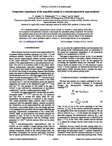
with 1/m1 = 1/mX + 1/mP , and 1/m2 = 1/mX − 1/mP . Parameters are chosen close to those of the experiments of ref. 4 in CdTe: exciton mass mX = 0.08me , photon mass mP = 2.58 × 10−5 me , ΩR = 26meV, and T2B = 13meV/1011 cm−2 . 1e+12

1e+11 -2

√ 2g ρ0

(To avoid the ultra-violet divergence associated with a delta-function interaction, the standard T-matrix renormalisation23 has been performed, thus T2B is the renormalised two-body T-matrix corresponding to the bare interaction g). In two dimensions, the BKT transition is found, as discussed above, by evaluating eq. (17) and eq. (19) at a fixed temperature, and finding the value of µ which satisfies limq→0 [χL (q) − χT (q)] = πkB T /2. The discussion up to now has been for a generic isotropic dispersion. For illustration, Fig. 2 shows the results of such a calculation with a dispersion appropriate to exciton-polaritons:   s  2 2 2 k 1 k − + Ω2R  , (20) f (k 2 ) =  2 2m1 2m2

Polariton Density (cm )

Γi (k + q, k) = γi (k + q, k)+

√
γi (q, 0) ρ0

Result of this article Method of Kavokin et al.

1e+10

1e+09

1e+08

1e+07

1

10

100

Temperature (K)

FIG. 2: Comparison of calculation of BKT critical density vs temperature for the method discussed here and the method in ref. 19,20. At low densities, both calculations agree, as nonquadratic effects are irrelevant, but where such effects matter, their predictions differ.

In the normal state, the transverse and longitudinal response functions should become equal. It is instructive to see how the expression for effective mass, weighting the density, appears in such a calculation. In the normal state, there are no condensate depletion effects to worry about, and so: Z dd k χL (0) = gk nB (f (k 2 )), (21) (2π)d The one-loop transverse response is as in eq. (17), but with ξk → ǫk = f (k 2 ). To see that they agree, it is convenient to rewrite eq. (17) with a change of integration variables. We first introduce x = k 2 , so dd k = Sd xd/2−1 dx/2,

4 with Sd the surface of the d-dimensional hypersphere, and then change integration variable again to f (x), with dx = df /f ′ (x), giving: Sd df xd/2−1 x(2f ′ (x))2 dnB (f ) (2π)d 2f ′ (x) 2 df   d h d/2 ′ i Sd df 1 2 x 2f (x) nB (f ) = d (2π)d 2f ′ (x) dx Z 2d dd k = gk nB (f (k 2 )), (22) d2 (2π)d

χT (0) = −

2 d Z

Z

where the second line is integration by parts, and the last used ∂x (2xd/2 f ′ (x)) = (d/2)xd/2−1 g(x). In conclusion, a formalism for calculating the transverse and longitudinal response functions of a Bose gas with arbitrary isotropic dispersion has been presented.

1 2

3

4

5

6 7

8

9

10

11

L. V. Butov, J. Phys.: Cond. Mat 16, R1577 (2004). L. S. Dang, D. Heger, R. Andr´e, F. Bœuf, and R. Romestain, Phys. Rev. Lett. 81, 3920 (1998). H. Deng, G. Weihs, C. Santori, J. Bloch, and Y. Yamamoto, Science 298, 199 (2002). M. Richard, J. Kasprzak, R. Romestain, R. Andr´e, and L. S. Dang, Phys. Rev. Lett. 94, 187401 (2005). J. P. Eisenstein and A. H. MacDonald, Nature 432, 691 (2004). J. P. Eisenstein, Science 305, 950 (2004). C. R¨ uegg, N. Cavadinin, A. Furrer, H.-U. G¨ udel, K. Kr¨ amer, H. Mukta, A. Wildes, K. Habicht, and P.Worderwisch, Nature 423, 62 (2003). M. Jaime, V. F. Correa, N. Harrison, C. D. Batista, N. Kawashima, Y. Kazuma, G. A. Jorge, R. Stern, I. Heinmaa, S. A. Zvyagin, et al., Phys. Rev. Lett. 93, 087203 (2004). T. Radu, H. Wilhelm, V.Yushankhai, D. Kovrizhin, R. Coldea, Z. Tylczynski, T. L¨ uhmann, and F. Steglich, Phys. Rev. Lett. 95, 127202 (2005). J. M. Kosterlitz and D. J. Thouless, J. Phys. C: Solid State Phys. 6, 1181 (1973). D. R. Nelson and J. M. Kosterlitz, Phys. Rev. Lett. 39, 1201 (1977).

A sum rule relates the longitudinal response to density weighted by effective inverse mass at a given momentum. Using such a formalism recovers the equivalence of transverse and longitudinal responses in the normal state. This formalism allows a consistent formulation of the critical conditions for the BKT transition in a twodimensional Bose gas.

Acknowledgments

I would like to thank F. M. Marchetti and M. H. Szymanska for the suggestion that lead to this work, and P. B. Littlewood for helpful discussion, and to acknowledge financial support from the Lindemann Trust.

12

13

14

15

16 17 18

19

20

21

22

23

D. R. Nelson, in Phase Transitions and Critical Phenomena, edited by C. Domb and J. Lebowitz (Academic Press, London, 1983), vol. 7, chap. 1, p. 2. D. S. Fisher and P. C. Hohenberg, Phys. Rev. B 37, 4936 (1988). H. T. C. Stoof and M. Bijlsma, Phys. Rev. E 47, 939 (1993). L. P. Pitaevskii and S. Stringari, Bose-Einstein Condensation (Clarendon Press, Oxford, 2003). Y. Takahashi, Nuovo Cimento 6, 371 (1957). J. C. Ward, Phys. Rev. 78, 182 (1950). A. Griffin, Excitations in a Bose-condensed Liquid (Cambridge University Press, Cambridge, 1994). A. Kavokin, G. Malpuech, and F. P. Laussy, Phys. Lett. A 306, 187 (2003). G. Malpuech, Y. G. Rubo, F. P. Laussy, P. Bigenwald, and A. V. Kavokin, Semicond. Sci. Technol. 18, S395 (2003). N. Nagaosa, Qauntum Field Theory in Condensed Matter Physics (Springer-Verlag, Berlin, 1999). J. Keeling, P. R. Eastham, M. H. Szymanska, and P. B. Littlewood, Phys. Rev. B 72, 115320 (2005). U. A. Khawaja, J. O. Andersen, N. P. Proukakis, and H. T. C. Stoof, Phys. Rev. A 66, 013615 (2002).