Sep 16, 2003 - In the above kz = âk2. 0 â k2 s where k2 s = k2 x +k2 y when the Weyl identity is used and k2 s = k2 Ï when the Sommerfeld identity is used.
Response of a Point Source Embedded in a Layered Medium W.C. Chew Center for Computational Electromagnetics and Electromagnetics Laboratory Department of Electrical and Computer Engineering University of Illinois, Urbana, IL 61801-2991 S.Y. Chen Agilent Technologies Inc. 3910 Brickway Blvd Santa Rosa, CA95403 September 16, 2003 Abstract This paper shows the equivalence of propagating plane waves due to a source through a layered medium using the recursive propagation approach and the slab approach. It points to errors in Equations (2.4.15) and (2.4.16) of [9], and corrects them. In addition, it proves that both of these solutions satisfy the reciprocity relationship. Furthermore, solution for odd and even symmetric sources in a layered medium is derived
1
Introduction
The propagation of waves through planarly layered medium is a subject of interest to the field of optics, geophysics, remote sensing, as well as in microwaves [1, 2, 3, 4, 5, 6, 7, 8, 9]. Layered medium is often used to make reflectors or Fabri-Perot resonators. Also, in order to calculate the scattering of particles or objects buried in a layered medium, one often has to find the Green’s function of a layered medium. Often time, a layered medium is an excellent approximation to a medium with an inhomogeneous profile. In this case, one approximates the inhomogeneous profile with a piecewise constant function, where the step size can be made very small. Hence, the solution of plane waves in a layered medium also provides an alternate solution to the ordinary differential equation governing the wave physics in an inhomogeneous profile. The Green’s function of a layered medium is often found by first expanding the field due to a point source in terms of plane waves propagating away from the point source. If the layering is orthogonal to the z direction as shown in Figure 1, then the point source field can always be expressed in terms of an integral linear superposition of plane waves using the Weyl identity [10]: eik0 r i = r 2π
∞ ZZ
dkx dky
−∞
1
eikx x+iky y+ikz |z| kz
(1)
or the Sommerfeld identity [9, 11]: eik0 r = r
Z∞
dkρ
0
p
kρ J0 (kρ ρ)eikz |z| kz
(2)
In the above kz = − ks2 where ks2 = kx2 + ky2 when the Weyl identity is used √ 2 2 and ks = kρ when the Sommerfeld identity is used. Here, k0 = ω µ0 ²0 = ω/c0 is the free-space wave number. Hence, given a point source in region m, to find the field in the other regions, we can use the above identities and reduce the problem to a 1D problem of plane waves propagating through a layered medium (in the case of Sommerfeld identity, it actually becomes a plane wave in the z direction, and cylindrical wave in the transverse direction). In the corresponding 1D problem, we can imagine a sheet source at z = z 0 , generating a bi-directional plane wave propagating through the layered medium. Once reduced to a 1D problem, there are two ways to find the field in region n given the source in region m. One is to recursively forward propagate the field from region m to region n. Another is to think of the layered medium between regions m and n to be a layered slab separating them. Then we can use the generalized reflection and transmission coefficient defined for the slab to derive an expression for the field in region n. We will show that these two methods are equivalent to each other. A large part of the knowledge needed to solve this problem is documented in [9]. However, there are errors in Equations (2.4.15) and (2.4.16) of [9] which will be corrected in this paper. k02
z �� ��� �
− d1 − d2
����� �
− dm−2
�� ��� � � ��� �� �
� ��� ��
z = z'
�� � �� � �
− dm−1 − dm − dm+1
− d N −2
��� �� � �
− d N −1
��� �� �
Figure 1: Geometry of a point source embedded in a layered medium.
2
Recursive Propagation Approach
Without loss of generality, we will assume that the field is an electromagnetic field of the transverse electric (TE) type, and assume that region n is below region m, or n > m. Generalization of these approaches to other types of field is quite straight forward. Using Equation (2.1.26) in [9], we can propagate the downward going wave in region m to region m + 1 easily. The formula that relates a downgoing wave in region i to a downgoing wave in region i − 1 at z = −di−1 is then given by iki−1,z di−1 − ikiz di−1 Si−1,i , = A− A− i−1 e i e
2
(3)
− is the same as Si−1,i defined in (2.1.26a) of [9], given here explicitly where Si−1,i as Ti−1,i , (4) Si−1,i = ˜ i,i+1 e2ikiz (di −di−1 ) 1 − Ri,i−1 R
where Tij and Rij are the Fresnel transmission and reflection coefficients, and for TE waves, they are µj kiz − µi kjz , µj kiz + µi kjz 2µj kiz Tij = 1 + Rij = , µj kiz + µi kjz
Rij =
(5)
˜ i,i+1 is the generalized reflection coefficient defined in [9] as while R 2iki+1,z (di+1 −di ) ˜ ˜ i,i+1 = Ri,i+1 + Ri+1,i+2 e , (6) R ˜ 1 − Ri+1,i Ri+1,i+2 e2iki+1,z (di+1 −di ) p In the above kiz = ki2 − ks2 where ks2 = kx2 + ky2 when the Weyl identity is used and ks2 = kρ2 when the Sommerfeld identity is used. The downgoing wave in region m can be shown to be : h i 0 ikmz z 0 ˜ m,m−1 M ˜ m, + e−ikmz (z +2dm−1 ) R A− (7) m = e
which is the same as Equation(2.4.12) in [9]. Applying (3) recursively, we obtain n−2 Y iknz dn−1 A− ej+1 Sj+1,j+2 eikmz dm Sm,m+1 = ne j=m
h
ikmz z 0
· e
where we have defined
i 0 ˜ m,m−1 · M ˜ m, + e−ikmz (z +2dm−1 ) R ej = eikjz (dj −dj−1 ) ,
(8)
(9)
which corresponds to the phase gained by the wave as it traverses a slab of thickness dj − dj−1 in the j-th layer. We can rewrite (8) as ikmz dm iknz dn−1 , = S˜mn− A− A− me ne
where
S˜mn− =
n−1 Y
j=m+1
ej Sj,j+1 Sm,m+1 .
(10)
(11)
S˜mn− can be thought as a generalized transmission coefficient in the downward direction where the effect of all layers are accounted for. One should refer to ref. [9] for more details on the above derivation, and the meanings of the different terms.
3
The Slab Approach
In the slab approach, we define a generalized transmission coefficient for the layered slab region separating regions m and n, the generalized transmission coefficient is given by [9] n−1 Y 0 0 Sm,m+1 ej Sj,j+1 , (12) T˜mn = j=m+1
3
where 0 = Si−1,i
Ti−1,i . 2 ˜0 1 − Ri,i−1 R i,i+1 ei
(13)
The above is similar to Equation (2.1.28) of [9]. It is to be cautioned that when we define the generalized transmission coefficient, the regions in m and ˜0 ˜ n become half spaces, and hence R i,i+1 in (13) is different from Ri,i+1 in (4). Furthermore, 0 = Tn−1,n . (14) Sn−1,n The derivation in [9] did not make this point clear, and hence, the Equations (2.4.15) and (2.4.16) there in are erroneous. Using the constraint condition that the downgoing wave in region n is a consequence of the transmission of the downgoing wave in region m plus the reflection of the upgoing wave in region n, we have 2iknz dn −iknz dn−1 ˜ 0 ikmz dm iknz dn−1 ˜ Rn,n−1 . + A− = T˜mn A− A− n Rn,n+1 e me ne
(15)
Solving (15), we have i−1 h 0 2 ikmz dm iknz dn−1 ˜ ˜ ˜ 1 − R R e . A− = T A− e n,n+1 n,n−1 n mn me n
(16)
i−1 h 0 0 ˜ n− ˜ n,n+1 R ˜ n,n−1 . M = 1−R e2n
(18)
˜0 ˜ It is to be noted that R n,n−1 above is different from Rn,n−1 . The former is the generalized reflection coefficient for the slab only while the latter is for the entire layered medium above region n. After using A− m from (7) into (8), we arrive at i h 0 −ikmz (z 0 +2dm−1 ) ˜ iknz dn−1 ikmz z 0 ˜ m eikmz dm , (17) ˜ ˜ ·M R = T M + e e e A− m,m−1 mn n n
where
When substituted in fully to find the field in region n, Equation (2.4.16) of [9] should read h i ˜ n,n+1 e−iknz dn−1 T˜mn eikmz dm F− (z, z 0 ) = e−iknz z + eiknz (z+2dn ) R i h 0 0 0 ˜ mM ˜ n− ˜ m,m−1 M , · eikmz z + e−ikmz (z +2dm−1 ) R z ∈ region n, z 0 ∈ region m, n > m,
z < z0.
(19)
Similarly, Equation (2.4.15) of [9] should read i h ˜ n,n−1 eiknz dn T˜mn e−ikmz dm−1 F+ (z, z 0 ) = eiknz z + e−iknz (z+2dn−1 ) R i h 0 0 0 ˜ mM ˜ n+ ˜ m,m+1 M , · e−ikmz z + eikmz (z +2dm ) R z ∈ region n, z 0 ∈ region m, n < m,
z > z0
,
(20)
h i−1 ˜0 = 1−R ˜0 ˜ n,n−1 e2 where M R . n+ n n,n+1 We can rewrite the above using the result of the recursive propagation approach, namely, by letting ˜ 0 = S˜mn− , T˜mn M n−
(21)
0 ˜ n+ T˜mn M = S˜mn+ .
(22)
4
4
Equivalence of the Two Approaches
The recursive propagation approach that yields expression (8) appears to be quite different from the slab approach that yields expression (17). In other words, the RHS and the LHS of (21) and (22) are very different in appearance. To show that they are equivalent, we define (0) 0 ˜ n− S˜mn = T˜mn M ,
(23)
˜ 0 is defined in Equation (18). where T˜mn is defined in Equation (12) and M n− We need to show that (0) S˜mn = S˜mn− , ∀n > m, (24) where S˜mn− is as defined in Equation (11), in order to show the equivalence of the two approaches. Before we prove the above, we need the following lemma. Lemma 1. The following formulas are equivalent to each other, namely: ´ ´³ ³ 2 ˜ i,i+1 R ˜0 ˜ i+1,i+2 Ri+1,i e2 1 − R e 1−R i,i−1 i i+1 ³ ´³ ´ 2 2 0 0 ˜ i+1,i+2 R ˜ ˜ = 1−R 1 − Ri,i+1 R (25) i+1,i ei+1 i,i−1 ei .
Proof. Using the fact that Rij = −Rji and that
2 ˜ ˜ i,i+1 = Ri,i+1 + Ri+1,i+2 ei+1 , R ˜ i+1,i+2 e2 1 − Ri+1,i R i+1
LHS
´ ³ 0 ˜ i,i−1 ˜ i+1,i+2 e2i+1 − Ri,i+1 + R ˜ i+1,i+2 e2i+1 R e2i 1 − Ri+1,i R Ã ! ³ ´ ˜0 Ri+1,i + R e2i i,i−1 2 2 0 ˜ i+1,i+2 e ˜ 1−R = 1 − Ri,i+1 R i+1 i,i−1 ei 2 ˜0 1 − Ri,i+1 R i,i−1 ei ³ ´³ ´ 0 0 ˜ i,i−1 ˜ i+1,i+2 R ˜ i+1,i = 1 − Ri,i+1 R e2i 1−R e2i+1
(26)
=
=
RHS.
(27)
The lemma is similar to Exercise 2.4 in [9]. Theorem 1. The recursive propagation approach and the slab approach are equivalent to each other, because (0) S˜mn = S˜mn− ,
∀n > m,
(28)
(0) where S˜mn and S˜mn− are as defined in (23) and (11)
Proof. The proof by induction is as follows. When n = m + 1, the equality is obvious. Next, assuming that (0) S˜mi = S˜mi−
then where
´−1 ³ (0) 2 ˜ i+1,i+2 R ˜0 e S˜m,i+1 = T˜m,i+1 1 − R , i+1,i i+1 T˜m,i+1
(29) (30)
³ ´−1 2 ˜0 e = T˜mi 1 − Ri,i+1 R ei Ti,i+1 i,i−1) i (0) = S˜mi
2 ˜ i,i+1 R ˜0 1−R i,i−1 ei ei Ti,i+1 . ˜0 1 − Ri,i+1 R e2 i,i−1 i
5
(31)
Consequently, (0) S˜m,i+1
³ ´−1 (0) 0 ˜ i+1,i+2 R ˜ i+1,i = S˜mi ei Ti,i+1 1 − R e2i+1 ´ ´−1 ³ ³ 0 0 ˜ i,i+1 R ˜ i,i−1 ˜ i,i−1 · 1−R e2i . · 1 − Ri,i+1 R e2i
(32)
But we can also show that
´−1 ³ ˜ i+1,i+2 Ri+1,i e2 . S˜m,i+1− = S˜mi− ei Ti,i+1 1 − R i+1
(33)
Consequently,
(0) S˜m,i+1 = S˜m,i+1−
(34)
if ´ ´³ 0 ˜ i,i+1 R ˜ i,i−1 ˜ i+1,i+2 Ri+1,i e2i+1 1 − R e2i 1−R ³ ´³ ´ 2 2 ˜ i+1,i+2 R ˜0 ˜0 = 1−R 1 − Ri,i+1 R i+1,i ei+1 i,i−1 ei . ³
(35)
The above equality follows from Lemma 1. Since (34) follows from (29) and that (28) is true when n = m + 1, the theorem is proved by induction.
5
Reciprocity Theorem
F (z, z 0 ) defined in [9] and in (19) and (20) is a solution to the following ordinary differential equation ¸ · 1 1 2 d 1 d + kz (z) F (z, z 0 ) = 2i kz δ(z − z 0 ), (36) dz µ(z) dz µ(z) µ(z) By going through similar procedure for proving the reciprocity theorem in electromagnetics [9, p. 20], we can show that, F (z, z 0 ) satisfies the following symmetry relation µ(z 0 ) µ(z) F (z, z 0 ) = F (z 0 , z), (37) kz (z 0 ) kz (z) which is also a reciprocity relationship. When applied to F+ (z, z 0 ) and F− (z, z 0 ) where the source and observation points are in different parts of the layered medium, the above relationship becomes µm µn F− (z, z 0 ) = F+ (z 0 , z), kmz knz
z < z0,
(38)
where z 0 ∈ Rm , z ∈ Rn , where Ri stands for region i. Consequently, in order for (19) and (20) to satisfy reciprocity, we require that µm ˜ ˜ mM ˜ n− = µn T˜mn M ˜ nM ˜ m+ , Tmn M kmz knz
(39)
The above is also the same as requiring µm ˜ ˜ m = µn S˜nm+ M ˜ n. Smn− M kmz knz
(40)
Theorem 2. Both the recursive propagation approach and the slab approach give rise to solutions that satisfy the reciprocity theorem.
6
Proof. Since Theorem 1 shows that both approaches are equivalent to each other, we need only to prove the validity of Equation (40). The factor on the LHS of (40) can be written as n−1 n−1 Y Y ˜m = ˜m ej S˜mn− M Sj,j+1 Sm,m+1 M j=m+1
=
We can rewrite −1 ˜m M
n−1 Y
j=m
³ ³
=
n−1 Y
j=m+1 n−1 Y
j=m+1
j=m+1
ej
ej
n−1 Y
j=m n−1 Y
˜m Sj,j+1 M
Tj,j+1 ˜ m . (41) M 2 ˜ 1 − R j+1,j Rj+1,j+2 ej+1 j=m
´ ˜ j+1,j+2 e2j+1 = 1 − Rj+1,j R ˜ m,m+1 R ˜ m,m−1 e2m 1−R
´ n−1 Y³ j=m
(42) ´
˜ j+1,j+2 e2j+1 . 1 − Rj+1,j R
Using a similar trick similar to Lemma 1, we rewrite the RHS of (42) as n−2 ´ ³ ´ Y ³ ˜ j+1,j Rj+1,j+2 e2j+1 1 − R ˜ n,n−1 R ˜ n,n+1 e2n 1−R j=m−1
n ³ Y
=
j=m+1
´
˜ n. ˜ j−1,j−2 Rj−1,j e2 M 1−R j−1
(43)
Now, if we look at the factor on the RHS of (40) n+1 m+1 Y Y ˜n ˜n = S˜mn+ M Sj,j−1 Sn,n−1 M ej j=n−1
j=n−1
=
n−1 Y
j=m+1
=
n−1 Y
j=m+1
ej
n Y
j=m+1
n Y
˜n Sj,j−1 M
Tj,j−1 ˜ n . (44) M 2 ˜ 1 − R j−1,j Rj−1,j−2 ej−1 j=m+1
ej
By using (32) and (33) in (31), we find that
Qn−1 n−1 Y Tj,j+1 ˜n S˜mn− M j=m Tj,j+1 Q . = = n ˜n T S˜nm+ M j=m+1 Tj,j−1 j=m j+1,j
(45)
For TE waves, by letting.
Tij =
2µj kiz , µj kiz + µi kjz
7
(46)
we have n−1 Y
n−1 Y µj+1 kjz Tj,j+1 = T µ k j=m j+1,j j=m j j+1,z
µm+1 kmz µm+2 km+1,z µn−1 kn−2,z µn kn−1,z · ... · µm km+1,z µm+1 km+2,z µn−2 kn−1,z µn−1 knz kmz µn . = µm knz
=
(47)
Consequently, (45) with (47) verifies (40).
6
Source Symmetry
Some sources produce an even symmetric field in the z direction about the source point z 0 in a homogeneous medium (we shall call them Type A sources), while others produce an odd symmetric field about the source point (we shall call them Type B sources). An example of the field produced by a Type A source is 0 F (z, z 0 ) = eikz |z−z | (48) while an example of the field produced by a Type B source is 0
Fo (z, z 0 ) = ±ikz eikz |z−z |
(49)
For instance, a horizontal electric dipole produces an even symmetric TE field, but an odd symmetric TM field about the source point [9, p. 73]. When the Type A source is placed inside a layered medium, the field it produces, F (z, z 0 ), satisfies (36). When a Type B source is placed inside a layered medium, the field it produces, Fo (z, z 0 ), can be easily derived from F (z, z 0 ) from the following theorem. Theorem 3. If a source produces an odd symmetric field in a homogeneous medium, the field it produces in a layered medium can be derived from F (z, z 0 ) that satisfies (36) by ∂ (50) Fo (z, z 0 ) = 0 F (z, z 0 ), ∂z Proof. The proof follows readily from differentiating (36) with respect to z 0 . Then we have ¸ · d 1 d 1 2 1 + kz (z) Fo (z, z 0 ) = −2i kz δ 0 (z − z 0 ), (51) dz µ(z) dz µ(z) µ(z) where
∂ F (z, z 0 ). (52) ∂z 0 In the above, we can exchange the order of differentiation because the differential operator in (51) does not depend on z 0 . When a medium is homogeneous, the above differential equation reduces to ¸ · 2 d 2 0 0 0 + k (53) z Fo (z, z ) = −2ikz δ (z − z ), dz 2 Fo (z, z 0 ) =
The above has a solution which is given by (49). Hence, Fo (z, z 0 ) is odd symmetric in a homogeneous medium, and in a layered medium, it satisfies the layered medium equation given by (51).
8
7
Conclusion
We have shown two equivalent ways to find the field at any layer due to a source embedded in a layered medium. Their equivalence are proved by mathematical induction. Furthermore, we show that the result obeys the reciprocity theorem. These two ways of finding the field due to a source can be used as alternative methods to solve for the solution of the ordinary differential equation governing the wave in a medium with an inhomogeneous profile. We also show how the solution that corresponds to a source that produces the odd-symmetric field can be derived easily from the solution for a source that produces an even-symmetric field by just a differentiation with respect to the source location. The results derived here can be used to find the field response of a point source embedded in a layered medium as described in [9].
References [1] L.M. Brekhovskikh, Waves in Layered Media, New York: Academic Press, 1960. [2] J.R. Wait, Electromagnetic Waves in Stratified Media, 2nd ed, New York: Pergamon Press, 1970. [3] J.A. Kong, “Electromagnetic field due to dipole antennas over stratified anisotropic media,” Geophysics, vol. 38, pp. 985-996, 1972. [4] L.B. Felsen and N. Marcuvitz, Radiation and Scattering of Electromagnetic Waves, New Jersey: Prentice-Hall, 1973. [5] K. Aki and P.G. Richards, Quantitative Seismology, Theory and Methods, vols. I and II, New York: Freeman, 1980. [6] L. Tsang, J.A. Kong, and R.T. Shin, Theory of Microwave Remote Sensing, New York: Wiley-Interscience, 1985. [7] P. Yeh, Optical Waves in Layered Media. New York: John Wiley & Sons, 1988. [8] M. Tygel and P. Hubral, Transient Waves in Layered Media, New York: Elsevier, 1987. [9] W.C. Chew, Waves and Fields in Inhomogeneous Media, Van Nostrand Reinhold, New York, 1990. Reprinted by IEEE Press, 1995. [10] M. Born and E. Wolf, Principles of Optics New York: Pergamon Press, 1980. [11] A. Sommerfeld, Partial Differential Equations in Physics, New York: Academic Press, 1949.
9