this class of applications and our main interest is in rule-based ... The result of missing a deadline in these ... RHS: the right-hand-side of a multiple assignment statement, and. 3. .... rule-based program and can thus avoid the state explo- sion. The new ... respect to the original one, the following properties: ⢠no cycles (all the ...
Response Time Optimization of Rule-Based Expert Systems∗ Blaˇz Zupan†, Albert Mo Kim Cheng Department of Computer Science University of Houston Houston, Texas 77204-3475 (blaz,cheng)@cs.uh.edu Abstract Real-time rule-based decision systems are embedded AI systems and must make critical decisions within stringent timing constraints. In the case the response time of the rule-based system is not acceptable, it has to be optimized to meet both timing and integrity constraints. This paper describes a novel approach to reduce the response time of rule-based expert systems. Our optimization method is twofold: the first phase constructs the reduced cycle-free finite state transition system corresponding to the input rule-based system, and the second phase further refines the constructed transition system using the simulated annealing approach. The method makes use of rule-base system decomposition, concurrency and state-equivalency. The new and optimized system is synthesized from the derived transition system. Compared with the original system, the synthesized system has (1) fewer number of rule firings to reach the fixed point, (2) is inherently stable, and (3) has no redundant rules.
1
Introduction
Modern, in particular computer based, technology is increasingly used in the environments where events are not predictable, the state of the world is not easily characterized in advance, and the time-response requirements are critical. Real-time systems belong to this class of applications and our main interest is in rule-based real-time systems and the problems posed by stringent time requirements these systems have to satisfy. The rise of the use of rule-based, real-time expert ∗ This material is based upon work supported in part by the National Science Foundation under Award No. CCR-9111563 and by the Texas Advanced Research Program under Grant No. 3652270. † On leave from “Joˇ zef Stefan” Institute, Ljubljana, Slovenia.
systems as embedded AI systems in different industrial applications, such as airplane avionics, smart robots, space vehicles and other safety critical applications increases the importance of the validation and verification phase of their life cycle. Apart from functional correctness, real-time expert systems must also satisfy stringent timing constraints. The result of missing a deadline in these systems may be fatal and the verification task is to prove that the system can deliver an adequate performance in a bounded time. If this is not the case or if the real-time expert system is too complex to analyze, the system has to be resynthesized. The definition of the synthesis problem given by Browne et al. in [2] is: “Given an equational rulebased program P that always reaches a safe fixed point in finite time but is not fast enough to meet the timing constraints under a fair scheduler, determine whether there exists an extension of P that meets both the timing and integrity constraints under some scheduler.” We propose a formal framework to a response-time optimization of the rule-based expert system given in the form of rule-based equational logic programs (EQL) as introduced by Browne et al. in [2] and Cheng and Wang in [6]. Our method is based on the identification of the finite state transition system for the original rule-based program. Because of the nontrivial nature of expert systems, the combinatorial explosion of states may threaten the implementability of such an approach. To tackle the complexity problem, we use several different approaches, the most important of them being: (1) the minimal model generation method by Bouajjani et al. [1], (2) the stubborn attack on state explosion using the notion of concurrency by Valmari [10], and (3) the equational program decomposition method and concurrent rule execution algorithm by Cheng [4]. Bouajjani et al. [1] proposes an algorithm for minimal model generation that can be used for building a state space graph of transition systems. The algorithm
combines generation and reduction methods. He uses a notion of the equivalency of states and instead of reducing a transition system from its non-reduced version introduces a unique approach of reducing the system during its generation. A stubborn attack on state explosion by Valmari is another method for state reduction. In [10] he argues that concurrency is the major contributor to state explosion. It introduces a large number of execution sequences that lead from a common start state to a common end state by the same transition, but the transition occurs in different order causing the sequences to go through different states. We use both approaches in combination with Cheng’s [4] parallel execution model. The later is used for rule-base system decomposition and reduction of complexity of optimization, and in combination with Valmari’s approach to reduce the number of states in the transition system. Since the proposed optimization usually increases the complexity of rules (enabling conditions), we introduce an additional optimization phase. It is based on the known method of simulated annealing [8] and attempts to reduce both the number of rules to be fired and the complexity of enabling conditions. The optimized rule-based system is synthesized from the derived transition system. The system is cycle-free and has optimal performance in terms of number of rules to be fired to reach the fixed point. The rest of the paper is organized as follows. In Section 2 we outline the syntax of EQL rule-based programs, introduce the transition system representation and describe the rule-based programs decomposition techniques. Section 3 describes the proposed optimization technique, which is ahen discussed in Section 4. The Additional optimization phase is described in Section 5. Section 6 is the conclusion.
2
environment
sensor readings
decisions
(input variables’ values) decision system
update of the system state (system variables’ values)
Figure 1: The real-time decision system. 2. RHS: the right-hand-side of a multiple assignment statement, and 3. EC: the enabling condition. An enabling condition is a predicate on the variables in the program. For ease of discussion, we define three sets of variables for a rule rk , 1 ≤ k ≤ M of an EQL program: 1. Lk = {v|v is a variable appearing in LHS of rk }, 2. Rk = {v|v is a variable appearing in RHS of rk }, and 3. Tk = {v|v is a variable appearing in EC of rk }. An example of an EQL program is shown below (Fig.2. We will restrict ourselves to the use of twovalued variables only. Note that EQL programs that use multivalued variables instead can be easily (automatically) converted to it. The assignment statements are interpreted from left to right.
Prerequisites
The real-time decision system investigated here is described by a model introduced by Browne et al. [2].The system interacts with the external environment by taking sensor readings and computing control decisions based on sensor readings and stored state information. This model is depicted in Fig.1. The decision system is represented as an equational EQL rule- based program [2, 3]. This consists of a finite set of M rules each of which has three parts: 1. LHS: the left-hand-side of a multiple assignment statement,
PROGRAM eql_program; INPUT b : boolean; VAR a, c : BOOLEAN; RULES (* 1 *) a:=TRUE IF NOT a AND b AND NOT a AND NOT b (* 2 *) [] c:=FALSE IF a AND c (* 3 *) [] a:=FALSE IF a AND b (* 4 *) [] a:=FALSE ! c:= TRUE END.
c OR AND NOT c AND NOT c IF a AND NOT c
Figure 2: An example of the EQL rule-based expert system.
The transition system of an EQL program, as defined in [2] is a labeled graph G = (V, E). V is a set of vertices each of which is labeled by a tuple: (x1 , ..., xn , s1 , ...sp ) where xi is a value in the domain of ith input sensor variable and sj is a value in the domain of the j th program variable. E is a set of edges each of which denotes the firing of a rule. An edge (i, j) connects vertex i to vertex j iff there is a rule r which is enabled at vertex i and firing r will modify the program variables to have the same values as the r tuple at vertex j. We will denote this with i→j. Fig.3 shows a transition system for a program in Fig.2. There are two vertices of special type (001 and 010) that have no outgoing edges and are said to be fixed points. Fixed points are states in the system where no rule is enabled or, if so, firing one will not change the state. Note that in our transition system r we do not mark the self loops, i.e. cycles of type i→i.
I.e. having two aggregate states I = {i1 , ..., im } and J = {j1 , ..., jm }, where i1 , ..., im , j1 , ..., jm are primir tive states, a relation I →J would mean that for every primitive state ix , x ∈ 1..m in I there exists primitive r state jy , y ∈ 1..n so that ix →jy . The parallelization of the rule-based system is interesting from the viewpoint of speeding-up the execution as well as for the decomposition of the system. Our main interest is in the later, since it makes the divide and conquer approach feasible to lower the complexity of the analysis and synthesis of the system. We refer to the parallel execution model proposed by Cheng [4]. He uses the notion of inter-ruleset parallelism to decompose the EQL program into inter-dependent rulesets. We use his model to optimize the rules in each such rule-set separately and thus decrease the complexity of the optimization phase.
3 000
101
1
2 100
111
1
2
4 110
4 001
011
3 010
Figure 3: A transition system for the EQL program in Fig.2. An invocation of an equational rule-based program can be thought of as tracing a path in the transition system. Every time the values of the input variables are changed (at that point the system is in a so-called launch state) the values of the system variables have to be determined through iterative firings of rules. The fixed point is reached when no variable’s value changes. The required property of hard real-time rule-based system is reaching the fixed point before the next change of the values of input variables. In accordance to this, Browne et al. [2] define a timing constraint as an upper bound on the length of the paths from a launch state to a fixed point, and this corresponds to the response time of the EQL program. The vertices of the above defined transition system describe a specific (and only one) state of the system. According to this we will also refer to them as primitive states. In the next section we will introduce the notion of equivalent states. These states will group equivalent primitive states into an aggregate states.
Method
Traditional methods [2] construct an expanded transition system that includes all the states and transitions and then use various reduction and optimization methods to construct a reduced transition system. They would then use the model checker for the temporal logic CTL [7] to check the integrity and timing constraints. This approach is potentially very complex because of the state explosion problem. Note that the system with N two-valued variables would have 2N different states. We here present an optimization method that derives the reduced transition system directly from the rule-based program and can thus avoid the state explosion. The new and optimized equational rule- based program is then synthesized from the derived transition system. Despite the fact that the reduced transition system can be used also for analysis purposes, our main goal is to use it for the synthesis of the new EQL program. The derived EQL program will have: • improved response time: if there would be two or more different paths from a launch state to the fixed point in the original non- reduced transition system, only the shortest one will be present in the reduced transition system, • no cycles: all states of the system are stable, and • no redundant rules/transitions. The method ensures the correctness of the derived expert system in terms of reaching the single accurate
expanded transition system derivation original equational rule-based program
transition system
transition system reduction
optimized derivation
reduced transition system rule-base synthesis
optimized equational rule-based program
Figure 4: Optimization of equational rule-base program. The steps taken by our optimization method are marked with solid line, while traditional and more complex optimization method is denoted by a dashed line. fixed point for each launch state. The semantics of the original system is altered since the method guarantees that a launch state will have just a single corresponding fixed point, which would be arbitrarily chosen from the set of original fixed points. To construct a reduced transition system, several techniques are combined. We first use a bottom-up derivation method, which starts from the fixed points and then gradually adds other states and transitions to the system. To decrease the complexity of the transition system, we identify the equivalent states while building the transition system. The third technique employs further reduction in the number of states and transitions combining those rules that can be fired in parallel. This section presents each of the above techniques and discusses the synthesis method.
3.1
procedure BottomU pDerivation() 1: T = {f | f is a fixed point } r 2: while (∃s 6∈ T and ∃s′ ∈ T so that s→s′ ) r ′ 3: add state s and transition s→s ) to T 4: end while
Bottom-Up Derivation of Transition System
Our bottom-up derivation starts at fixed points of the system and gradually builds the transition system iteratively adding new states. Each state is added to the system only once, and the resulting transition system will thus have states/vertices with at most one outgoing transition/edge. The algorithm is depicted in Fig.5. In the above algorithm, the states used for the expansion of the current transition system are arbitrarily chosen. Each original (expanded) transition system
Figure 5: Bottom-up derivation of transition system. may thus have different corresponding bottom-up constructed transition systems. We do not construct the transition system from the existent (expanded) one but rather use the rule-based program and a set of corresponding fixed points. Therefore, we have to apply the rules “in reverse manner”, meaning that given the state s′ and rule r we have to find a state s so that r s→s′ ). We have developed a set of functions that allow us to do so. Interested reader should refer to [11] for a detailed description. Fig.6 shows an example of the original and corresponding bottom-up transition system, which has, in respect to the original one, the following properties: • no cycles (all the cycles from the original transition system are removed), • determinism: each state has only one corresponding fixed point, • the states that do not have a path to any of the fixed points are eliminated, and • substantial number of transitions are eliminated. To reduce the response time we can combine the bottom-up derivation with the breadth-first search approach. We assume the fixed points to be at level 0 and other states to be at level l, where l is a number of transitions between the specific state and its corresponding fixed point. Breadth-first search technique will add all the lower level states to the transition system prior to the higher level states. Such derivation will result in constructing only the shortest paths from a certain state to its corresponding fixed point.
3.2
Equivalent States
Our bottom-up derivation reduces the number of states in the transition system by excluding the states that do not have a corresponding path to the fixed points. The number of states can be further reduced with combining the equivalent states into the single aggregate state. We follow the idea of Bouajjani et al. In [1] they proposed an algorithm which, instead
(A) a
b
1
2 c
d
3 2
e
a
h
k
i
c
3 f
m
d
k
l
4
3 e
f
4 m
j 2
d
3
l 3
(B)
2
j 2
1
4
2
f
c
b
j 4
2
3
b
1
e
g
a
5
k
l 3
m
4
Figure 7: Transition system with grouped equivalent states constructed from the system in Fig.6.A.
3.3 Figure 6: An example of original (expanded) transition system (A) and corresponding bottom-up constructed transition system (B).
of reducing a transition system from its non-reduced version, performs a reduction during its generation. We use the algorithm proposed by Bouajjani et al. and combine it with breadth-first search derivation. The initial transition system consists of a single aggregate state which includes all the fixed points. Again, the transition system is gradually expanded, this time grouping all the states that lead to the same aggregate state using a specific transition. I.e., having a state I ∈ T , where T is a current transition system under generation, we can expand T with aggregate r state J and transition r, so that I →J. All the aggregate states in the new transition system have to be mutually exclusive, i.e. 6 ∃s . s ∈ I ∧ s ∈ J . I 6= J, where s is some primitive state and I and J are aggregate states in the transition system. As before, we use the breadth-first search technique. We also use a heuristic technique that adds to the transition system first those aggregate states that include the highest number of primitive states. Ties are broken arbitrarily. Fig.7 shows a transition system with equivalent states grouped into aggregate states that corresponds to the transition system from Fig.6. The number of states in the transition system is reduced from 10 to 5, while the original non- reduced transition system included 13 states.
Reduction of Transition System Due to Rule Execution Concurrency
The transition systems introduced above have single-rule transitions. We here present a method that can generate a transition system with transitions labeled with one or more rules (multiple- rule transitions). Suppose we have two aggregate states I and J, and a set of rules R = {r1 , ..., rk } that are all enabled at I, i.e. ∀ri ∈ R . ∃s ∈ I so that ri is enabled at s. We R r can write I →J) if ∀s ∈ I . ∃s′ ∈ J so that s→s′ . For rules in R we impose the following constraints: C1. rules in R can be fired in parallel, and C2. firing the rules in R should not result in a cycle that would include only the primitive states in I. For two rules ra and rb both belonging to R, the formalization of the above constraints is: D1. rule ra and rb do not potentially disable each other, D2. La ∩ Lb = ∅, or La ∩ Lb 6= ∅ and the same expression is assigned to the variables of the subset, and D3. La ∩ Rb = ∅ and Lb ∩ Ra = ∅. D1 follows the idea of intra-ruleset parallelism introduced by Cheng [4] (C1), and D2 and D3 guarantee the cycle- freedom (C2). The transition system generation algorithm is now more complex so that not only all the states of the certain level would be considered for the expansion, but also all the possible combinations of rules satisfying D1 to D3 would have to be derived and used. Having an aggregate state S ∈ T that is considered
for expansion, and a group of rules R, so that each of its firing can result in S, we construct concurrent execution graph CON(V, E). Each vertex in CON represents a single rule from R and two vertices are connected if D1 to D3 hold for corresponding two rules. From the graph CON we construct all possible combinations of rules that can be fired in parallel. The algorithm uses the matrix M representation of CON, where the size of M is |R|2 and M is defined as: � 1 if i and j are neighbors in CON Mi,j = 0 otherwise The algorithm removes all equal rows and rows that include all corresponding 1’s of some other row. Each row of the resulting matrix represents a group of rules to be fired in parallel. Thus, for row i, rules rj can be fired in parallel iff Mi,j = 1. In the transition system construction algorithm (Fig.10) we will denote this procedure with G(CON). Rx ∈ G(CON) would be one of possible rule-sets to be used in a transition.
Considering our example transition system from Fig.7 and knowing that rules 3 and 4 satisfy the constraints D1 to D3, whiles rules 1 and 2 do not, we can construct the reduced transition system as shown in Fig.9.
a 1
4
1
2
Figure 8: An example of CON graph. We here show an example of the derivation of G(CON). Suppose we have a CON graph for four rules shown in Fig.8. The initial M matrix is:
1
1 2
3 4
1 1
1 0
2 1 1 M= 31 1 4
0 1
1 1 1 1 1 1
and the resulting matrix is:
M=
1 2
3 4
3
1 1
1 0
4
0 1
1 1
!
Therefore, G(CON) = {{1, 2, 3}, {2, 3, 4}} and the transition may be labeled with rules 1, 2 and 3, and 2, 3 and 4.
j 2
c
d
k
l
{3,4} e
f
m
Figure 9: A transition system with multiple-rule transitions and aggregate states.
3.4 3
b
Transition System Construction: The Algorithm
The algorithm that combines the approaches introduced above and builds the reduced transition system directly from the original rule- based EQL program is depicted in Fig.10. Variables States and Edges store the current state of the transition system. T oExpand stores the states that are considered to be expanded. Initially, T oExpand consists of a single aggregate state that includes all the fixed points. N extT oExpand stores the states of the next level. In each iteration an aggregate state that stores the biggest number of primitive states is chosen for the expansion. If there is no such state (state includes 0 primitive states), T oExpand becomes N extT oExpand and the next level of states is investigated. The derivation terminates when there are no more states available to expand. Cover includes all the primitive states currently in the transition system and is used to obtain aggregate states that are mutually exclusive (line 12 in the algorithm). Despite the fact that the use of multiple-rule transitions reduces the number of states, there is a certain advantage of single-rule transitions systems. Namely, the latter are always deterministic, meaning that at each primitive state of the system at most one rule will be enabled. It has been shown [11] that it is easy to convert multiple-rule transitions system to the one
procedure T ransitionSystem() 1: States := FixedPoints(); Cover := States; Edges := ∅ 2: T oExpand := State; N extT oExpand := ∅ 3: repeat 4: repeat 5: forall S ∈ T oExpand do r 6: Applicable := {ri : ∃S ′ . S →S ′ )} 7: for rules in Applicable construct CON graph 8: forall R ∈ G(CON) do r ′ 9: SS,R := ∪ S ′ − Cover where S →S ′ , r ∈ R 10: end forall 11: end forall ′ | = Max 12: chose S ′ S,R so that |SS,R ′ 13: if |SS,R |= 6 0 then R
′ 14: Edges := Edges ∪ SS,R →S ′ 15: States := States ∪ {SS,R } ′ 16: Cover := Cover ∨ SS,R 17: N extT oExpand := N extT oExpand ∪ S ′ S,R 18: end if ′ 19: until |SS,R |=0 20: ToExpand := NextToExpand 21: until T oExpand = ∅
Figure 10: Bottom-up breadth-first search construction of reduced transition system. with single-rule transitions, and we may use two different approaches in combination.
3.5
Synthesis of an Optimized RuleBased System
A new EQL program is synthesized from the constructed T R s. For each rule in a independent rule-set we determine the new enabling condition by scanning through T R so that for rule i, _ ECiN ew = ( So ) ∧ ECi i
So →Sd
New rules are then formed with the same assignment parts as in the original rules and new enabling conditions.
4
Discussion
It was shown [12] that the proposed algorithm can be applied to minimize the number of rule firings. The method was used to optimize a set of randomly generated EQL programs of up to 15 rules and up to 10 variables. The Estella - General Analysis Tool proposed
by Cheng et al. [5] was used to estimate the response time in regard to the number of rule firings for the original programs. The same metrics were derived directly from the transition systems using the proposed optimization algorithm for the optimized programs. While the optimized programs required on the average 25% to 50% fewer rule firings to reach the fixed point, the enabling condition complexity increased up to 2000%. The algorithm was also used to optimize the Integrated Status Assessment Expert System (ISA) [9]. We used the two-valued EQL version with 35 rules and 58 variables. The Estella - General Analysis Tool [5] was used to determine the stability of the system and discovered several cycles which led to a termination of the analysis. Thus, the time response of the original program could not be determined and the authors are unaware of any other method that could do so. Still, we have used the ISA expert system to compare the complexity of the unoptimized and optimized programs, and discovered that the later has approximately 10 times more complex enabling conditions. All this led us to believe that optimization should also address enabling condition complexity and that the response time should not be viewed solely from number of rule firings point of view.
5
Proposal for Additional Iterative Improvement Method
In the previous sections we have shown the optimization technique, which improves the input rulebased program in different ways, but addresses the response time only from the viewpoint of the upper bound of number of rules to fire to reach the fixed point. The optimization process makes the rules’ enabling conditions more specific than the original ones and thus increases their complexity. The proposed optimization does not address this issue. Here we introduce the method that attempts to minimize both the number of rules to fire and the complexity of enabling conditions. The iterative improvement method introduced here starts from the transition system derived by our optimization algorithm and attempts to iteratively improve it. The improvement is defined by means of minimizing the cost function. In each iteration, the method generates a new transition system from the old one and synthesizes the corresponding EQL program. It then compares the cost of both solutions, and if the acceptance criteria is satisfied accepts a new solution.
Owing to its simplicity and potentially good performance [8] we use a simulated annealing optimization method scheme. keep with current solution from the derivation of optimized transition system
transition system
neighboring solution
the new solution is the neighbor
no accept the neighbor?
yes
Figure 11: Iterative improvement method. Fig.11 describes the iterative improvement method. The cost function to be minimized by the simulated annealing program is C = c1 N RF + c2 ECC + c3 (N S − N S0 ) where N RF is the maximum number of rules to fire to reach a fixed point, ECC represents the complexity of the enabling conditions, N S is the number of states of the newly derived transition diagram, and N S0 is the number of states in the original transition diagram (output of the greedy or breadth-first algorithm from the previous section). ECC is expressed as the average number of two-valued operations (AND, OR, NOT) to evaluate the enabling condition. Constants c are weights and depending on the type of the optimization preferred can be set accordingly. The critical phase of the algorithm is derivation of the neighboring solution. The main idea is to steal some primitive states from certain aggregate state of the system and either add them to some other aggregate state or create a new aggregate state. The main constraints for the method are that: (1) the resulting system has to be correct, (2) it is cycle-free, and (3) all the primitive states present in the original system have to be present in the neighboring one. The algorithm for derivation of the neighboring solution is rather complex and lengthy to describe and is presented in detail in [11]. We are currently working on the implementation and evaluation of the impact of such an algorithm.
6
Conclusion
We have presented a new two-phase algorithm for the response time optimization of rule-based expert system. The two-phase algorithm first constructs the
reduced and optimized transition system, which encodes all the necessary information about the behavior of the real-time system. Next, the corresponding optimized rule-based system is constructed from the derived transition system. The original and optimized rule-based systems are equivalent: all the launch states of the optimization system reach exactly one corresponding fixed point from the original system. Furthermore, the new system is stable and does not contain cycles, and has optimal performance in respect to the number of rules to fire to reach a fixed point. The proposed optimization technique would usually increase the complexity of enabling conditions and this might influence the response time of the rulebased program. We propose an additional optimization phase based on the known optimization method of simulated annealing. This uses the derived reduced transition system and attempts to change it so as to minimize both the number of rules to be fired and the complexity of the enabling conditions.
References [1] A. Bouajjani, J.-C. Fernandez, and N. Halbwachs. Minimal model generation. In E. M. Clarke and R. P. Kurshan, editors, Proc. of 2nd International Conference, CAV ’90, pages 197– 203, New Brunswick, NJ, June 1991. SpringerVerlag. [2] J. C. Browne, A. M. K. Cheng, and A. K. Mok. Computer-aided design of real-time rule-based decision system. Technical report, Department of Computer Science, University of Texas at Austin, 1988. Also to appear in IEEE Trans. on Software Engineering. [3] A. M. K. Cheng. Analysis and synthesis of realtime rule-based decision systems. PhD dissertation, Dept. of Computer Science, University of Texas at Austin, 1990. [4] A. M. K. Cheng. Parallel execution of real-time rule-based systems. In Proc. of IEEE International Parallel Processing Symposium, pages 779– 789, NewPort Beach, CA, April 1993. [5] A. M. K. Cheng, J. C. Browne, A. K. Mok, and R.-H. Wang. Analysis of real-time rule-based system with behavioral constraint assertions specified in Estella. IEEE Trans. on Software Eng., 19(19):863–885, September 1993.
[6] A. M. K. Cheng and C.-K. Wang. Fast static analysis of real-time rule-based systems to verify their fixed point convergence. In Proc. 5th Annual IEEE Conf. on Computer Assurance, pages 197– 203, NIST, Gaithersburg, Maryland, June 1990. [7] E. M. Clarke, E. A. Emerson, and A. P. Sistla. Automatic verification of finite-state concurrent system using temporal logic specifications. ACM Trans. on Programming Languages and Systems, 8(2):244–263, April 1986. [8] S. Kirkpatrick, C. D. Gelatt, and M. P. Vecchi. Optimization by simulated annealing. Science, 220:671–680, 1983. [9] C. A. Marsh. The ISA expert system: A prototype system for failure diagnosis on the space station. MITRE report, The MITRE Corporation, Houston, Texas, 1988. [10] A. Valmari. A stubborn attack on state explosion. In E. M. Clarke and R. P. Kurshan, editors, Proc. of 2nd International Conference, CAV ’90, pages 156–165, New Brunswick, NJ, June 1991. Springer-Verlag. [11] B. Zupan. Optimization of real-time rule-based systems using state-space diagrams. Master’s thesis, University of Houston, Department of Computer Science, 1993. [12] B. Zupan and A. M. K. Cheng. “Optimization of rule-based systems via state transition system construction”. to be presented at IEEE Conf. on Artificial Intelligence for Applications, March 1993.