three-body problem (R3BP), and named it the restricted full three- body problem ... and final conditions at the surface are crucial for designing transfer maneuvers of a .... The free parameters of this system are the mass ratio, , the distance ...
JOURNAL OF GUIDANCE, CONTROL, AND DYNAMICS Vol. 31, No. 1, January–February 2008
Restricted Full Three-Body Problem: Application to Binary System 1999 KW4 Julie Bellerose∗ and Daniel J. Scheeres† University of Michigan, Ann Arbor, Michigan 48109 DOI: 10.2514/1.30937 The motion of a satellite in the gravitational field of a binary system is investigated. The two bodies of the binary system are modeled as a sphere and a triaxial ellipsoid and the satellite is assumed to have no influence on the motion of the two primaries. The case of relative equilibria in the full two-body problem is assumed. In earlier papers, we looked at equilibrium solutions in the restricted full three-body problem, especially for L4;5 . In the present work, we investigate energy constraints on the motion of the spacecraft using zero-velocity curves, collinear Lagrangian points, and the Jacobi constant for varying parameters of the system. We study transit and nontransit trajectories between the components. The methods are applied in the study of the binary asteroid system 1999 KW4, and some results are shown.
Looking at the case of L1 especially, if the zero-velocity curves are open, this implies that particles could transit from one body to the other. This problem has interesting application to surface vehicles transiting between the binary components. As rovers are now sent to investigate small bodies to get samples back to Earth, such as the JAXA’s Hayabusa mission [6], surface motion on both bodies and transfers between them are important to consider in the design of missions to a binary system. In this case, however, because of the unstable nature of L1 , only specific regions and conditions at the body surface can lead to transit or nontransit trajectories. The initial and final conditions at the surface are crucial for designing transfer maneuvers of a vehicle. These findings can also give us a better understanding of particles dynamics near the surface. In the following sections, we first review the dynamics of the binary system itself before looking at the motion of a particle in this gravitational field in more detail. Finally, we apply these theoretical developments to a recently analyzed binary system, designated Asteroid 1999 KW4 [5].
I. Introduction
I
N RECENT years, we have witnessed a few spacecraft missions sent to small bodies of our solar system. With the growing interest in asteroid systems in the scientific community, it is fair to assume that a mission will target a binary asteroid system in the near future. To develop a model suitable for binary asteroid systems, we took into account the mass distribution of one of the bodies of the restricted three-body problem (R3BP), and named it the restricted full threebody problem (RF3BP). The “full” problem has proven to be a dynamically rich problem. Previous papers have considered relative equilibria of the binary itself, or the full two-body problem (F2BP) [1,2] and stability of equilibrium solutions in the RF3BP [3,4]. In [1], the author discusses the stability region of the relative equilibria for an ellipsoid-sphere system; it is common to find systems made of a small ellipsoid and a large sphere [5]. Scheeres [2] gives a more general discussion on the conditions for equilibria in the general case of the F2BP under sphere restriction. In the case of the RF3BP, [3] derived the general equations of motion of a particle in the RF3BP, whereas Bellerose and Scheeres [4] looked at equilibrium solutions for an ellipsoidsphere system. In particular, the stability of the equilateral Lagrangian points have been investigated. It was found that the ellipsoid reduces the stability region compared with the R3BP. In the present work, we give a more general discussion of the equilibrium solutions and the energy constraints associated with them for an ellipsoid-sphere system. In the case of an equilibrium in the F2BP, the system allows for one integral of motion, the Jacobi integral. As for the R3BP, different values of the Jacobi integral lead to the definition of the Lagrangian points, in which the regions of allowable motion can be mapped. For particular values of the free parameters of the system, we solve for the collinear Lagrangian points. Because the mass distribution of one of the bodies is taken into account, the system has an extra physical constraint in that Lagrangian points should be located outside of the body.
II.
Full Two-Body Problem
Before defining the dynamics for a particle in orbit about a binary system, we need to address the full two-body problem itself. We consider an ellipsoid-sphere system. The general problem is represented in Fig. 1. In this model, M1 is the mass of the spherical shape and M2 is the mass of the ellipsoid. The mass ratio of the two primaries is defined as ��
M1 M1 � M2
(1)
We use r b for the position vector of the sphere relative to the ellipsoid. Relative to their center of mass, we also have the positions
Presented as Paper 224 at the AAS Spaceflight Mechanics Meeting, Sedona, Arizona, 28 January–1 February 2007; received 14 March 2007; revision received 1 August 2007; accepted for publication 1 August 2007. Copyright © 2007 by the American Institute of Aeronautics and Astronautics, Inc. All rights reserved. Copies of this paper may be made for personal or internal use, on condition that the copier pay the $10.00 per-copy fee to the Copyright Clearance Center, Inc., 222 Rosewood Drive, Danvers, MA 01923; include the code 0731-5090/08 $10.00 in correspondence with the CCC. ∗ Ph.D. Candidate, Department of Aerospace Engineering. Student Member AIAA. † Associate Professor, Department of Aerospace Engineering; scheeres@ umich.edu. Associate Fellow AIAA.
r e � ��rb
(2)
r s � �1 � ��rb
(3)
where subscripts s and e refer to the sphere and the ellipsoid, respectively. Taken from [1] for a general body in a sphere restricted binary system, the dynamics of the binary system in the general body-fixed frame is defined by ~ _ � rb � � � �� � rb � � G�M1 � M2 � @U r� b � 2� � r_b � � @rb (4) 162
163
BELLEROSE AND SCHEERES
M2
Izz � 15�1 � �2 �
M1
ω CM re
rs
Fig. 1 Representation of the full two-body problem for an ellipsoidsphere system.
and the rotational dynamics of the general body are described in the general body-fixed frame by _ � �I � � � �GM1 rb � I ��
@U~ @rb
(5)
where � is the angular velocity of the general body, I is its inertia matrix normalized by its mass and U~ is the mutual potential, defined as Z 1 dm2 ��� (6) U~ � M2 �2 jrb � �j The variable � is the position vector of a mass element of the general body. To simplify the analysis, the following normalizations are introduced. The maximum radius of the distributed body, denoted by �, and the mean motion of the system at this radius r��������������������������� G�M1 � M2 � n� �3 are taken as length and time scales, respectively. The normalized position and angular velocity are then r�
rb �
!�
and
From Eqs. (7) and (8), we can solve for relative equilibria when all first and second derivatives are zero. With these same equations, it is then possible to show that there exists equilibria when one of the principal axes of the ellipsoid is pointed at the sphere, as the acceleration and position vectors are parallel. Similarly, we can show that the spin vector is perpendicular to the position vector, and it is parallel to one of its principal axes. These equilibria are independent of the principal axis the ellipsoid is rotating about; solutions exist along the x, y, and z axis. Given a solution along a q axis, which can be x, y, or z, the square of the spin rate is expressed as[3]
� n
!2 �
3 2
Z
1 �
dv ��2q � v���v�
(12)
Note that the spin may be about one of the other two principal axes. For the present problem, �q represents the radius along which the sphere is located. Note that here, � � q2 � �2q , in which q is the distance between the primaries. In our analysis, we denote q as r, with the ellipsoid having �q � � � 1. The relative equilibria for an ellipsoid-sphere system and their stability have been mapped in [1] as a function of the mass ratio and distance between the bodies. This work studied two configurations in which the � or � ellipsoid parameter is aligned with the sphere, referred to as the long-axis and short-axis configurations, respectively. We choose to consider the long-axis configuration, as it was shown to be the only energetically stable configuration for certain parameters. Hence, in Eq. (12), we look at the case in which r is along the x axis. Note that following a more general discussion of the F2BP in [2], the spectral and energetic stability of the ellipsoidsphere system relative equilibria were also studied for the case of a fixed value of angular momentum [8]; however, this topic is not addressed in the current paper.
and Eqs. (4) and (5) now become r� � 2! � r_ � !_ � r � ! � �! � r� �
I � !_ � ! � I � ! � ��r �
@U @r
@U @r
III. (7)
(8)
In this work, we model the general body as an ellipsoid. As discussed in [7], the general expression for an ellipsoid potential energy is written in terms of elliptic integrals. The mutual potential can be expressed as Z 3 1 dv (9) ��r; v� Ue � 4 � ��v�
��r; v� � 1 �
��v� �
x2 y2 z2 � � 2 v�1 v�� v � �2
p��������������������������������������������������� �v � 1��v � �2 ��v � � 2 �
(10)
A.
Restricted Full Three-Body Problem
Equations of Motion of a Particle
Having a relative equilibrium state in the F2BP, we look at the dynamics of a particle in this gravitational field. Earlier studies looked at equilibrium solutions, especially the equilateral Lagrangian points and their stability [4]. By investigating the collinear points, zero-velocity curves and the Jacobi integral, one can give a general description of the constraints on a particle’s dynamics. We now consider a particle or a spacecraft in the gravitational field of the binary system. For the current problem, we assume relative equilibrium of the F2BP as defined by Eqs. (7) and (8). The equations of motion of a particle were originally defined in [3]. As shown in Fig. 2, we now let � be the position of a particle relative to the center of mass of the system. The dynamics are expressed as �� � 2� � �_ � � � �� � �� � G�M1 � M2 �
(11)
where 0 < � � � � 1 and � satisfies ��r; �� � 0. In this work, the x axis is aligned with the longest axis of the ellipsoid , whereas the z axis is along its shortest axis. The normalized principal moments of inertia are Ixx �
1 2 �� 5
ρ y
M2
Iyy � and
M1
ω
2
�� �
CM 1 �1 5
@U~ 12 @�
x
2
�� �
re
Fig. 2
rs
The restricted full three-body problem.
(13)
164
BELLEROSE AND SCHEERES
In normalized units, Eq. (13) becomes
!2 y �
@U ~ � 12 ��~ � 2! � �_~ � ! � �! � �� @�~
(14)
where �~ �
� �
is the normalized distance of the particle. Because we take a frame fixed to the ellipsoid, U12 is a time-invariant potential energy expression, as the bodies are in mutual equilibrium. It is expressed as U12 �
� � �1 � ��Ue ��~ � �r� j�~ � �1 � ��rj
(15)
Ue represents the normalized expression for the ellipsoid body, defined by Eqs. (9–11). The free parameters of this system are the mass ratio, �, the distance between the two bodies, r, and the size parameters of the ellipsoid, � and �. Given these parameters, the spin rate ! is given by Eq. (12). The equations of motion can be restated in an �x; y; z� coordinate system; that is, �~ � xi � yj � zk. The x, y, and z components of Eq. (14) are written as follows: x� � 2!y_ � !2 x �
�� x � �1 � ��r
3 f x � �1 � ��r 2 � y2 � z2 g2
� �1 � ���x � �r�Rj� y� � 2!x_ � !2 y �
z� �
��z 3 � �1 � ���z�Rj� f x � �1 � ��r 2 � y2 � z2 g2
(18)
The Rj expressions are elliptic integrals taking into account the mass distribution of the ellipsoid. They are given in the Appendix. B.
Equilibrium Solutions
As for the R3BP, five equilibrium solutions exist when velocities and accelerations are set to zero in Eq. (14), and are solutions of the equation ~ � ! � �! � ��
@U12 @�~
(19)
These five locations are shown qualitatively in Fig. 3. The equilibrium solutions are then computed from !2 x �
� x � �1 � ��r
3 � �1 � ���x � �r�Rj� f x � �1 � ��r 2 � y2 � z2 g2
(20)
(21)
where ! is given by Eq. (12). These algebraic equations were solved numerically using MATLAB for varying free parameters. Note that z � 0 in all cases. The Lagrangian points can also be defined using the Jacobi integral of the system. This topic is introduced in the next section. C.
Spectral Stability
In the R3BP, for all values of the free parameters, L1 , L2 , and L3 are unstable, whereas L4;5 may be stable. Looking at small deviations from the equilateral position, we can investigate their stability. In the R3BP, the stability criteria for L4;5 is usually given by the Routh criteria and is only function of the mass ratio: " r������� 1 23 1� � 0:0385 . . . (22) �< 2 27 Because the mass distribution of the general body is now taken into account, the stability of some of the equilibrium solutions are expected to deviate from the R3BP. We introduce x � x~ � dx and y � y~ � dy, and expand the potential energy expression. The following equations are derived:
(16)
��y 3 � �1 � ���y�Rj� f x � �1 � ��r 2 � y2 � z2 g2 (17)
�y 3 � �1 � ��yRj� f x � �1 � ��r 2 � y2 � z2 g2
~ xxs � Uxxe � � y�U ~ xys � Uxye � x�~ � 2!y_~ � !2 x~ � x�U
(23)
~ yys � Uyye � � x�U ~ yxs � Uyxe � y�~ � 2!x_~ � !2 y~ � y�U
(24)
The second order partial derivatives for the ellipsoid potential were given in [1]. The characteristic equation for the system is found from � � 2 � � � !2 � Uxx �2!� � Uxy � ��0 � (25) � 2!� � Uxy �2 � !2 � Uyy � where Uxx � Uxxs � Uxxe , Uyy � Uyys � Uyye , and Uxy � Uxys � Uxye . Expanding the determinant, the characteristic equation is found to be of the form �4 � A�2 � B � 0
(26)
A � 2!2 � Uxx � Uyy
(27)
2 B � !4 � !2 �Uxx � Uyy � � Uxx Uyy � Uxy
(28)
where
and
For the system to be linearly stable, the following conditions must be satisfied: A>0
(29)
B>0
(30)
A2 � 4B > 0
(31)
L4
L3
L1
L5
Fig. 3
The analog Lagrangian points.
L2
As in the R3BP, the collinear Lagrangian points L1;2;3 are unstable. The equilateral Lagrangian points were studied in [4]. For these, the stability was found to be decreased from the known R3BP (also see Fig. 7). We give a more detailed description of L4;5 with the discussion on energy constraints in the next section.
165
BELLEROSE AND SCHEERES
3
IV. Energy Constraints A.
Jacobi Integral 2
With the two bodies being in relative equilibrium, this system allows for one integral of motion, the Jacobi integral. For a spacecraft navigating in this system, computing its Jacobi integral value is important, as it indicates the regions in which it can move and provides necessary conditions for when it may escape the system. To compute the integral, let us rewrite Eqs. (16) and (17) in the following form: x� � 2!y_ �
@V @x
(32)
y� � 2!x_ �
@V @y
(33)
* L4 1
L 3*
y 0
* L5 −2
(34)
where V��
� 1 � Ue �� � re � � !2 �x2 � y2 � j� � rs j 2
(35)
with rs �
p��������������������������������������������� f x � �1 � ��r 2 � y2 g
and Ue � 32�1 � ��Rj0 � 12�1 � �� �x � �r�2 Rjx � y2 Rjy
To derive the Jacobi integral, we multiply each of the two previous _ respectively, and add them up to find equations by x_ and y, _ � yy� _ � x� x_ �y� y_ ��z z_ �!2 �xx
@V @V @V x_ � y_ � z_ @x @y @z
(36)
We substitute x� �
dx_ dx_ dx � dt dx dt
and integrate with respect to time. Equation (36) becomes C � 12�x_ 2 � y_ 2 � z_2 � � V
−1
B.
2
3
xL1 � 1 � �r
(42)
1 0.8 0.6 0.4 0.2 y
y
(39)
0
*
−0.2 −0.4
(40)
L1
−0.6 −0.8
And we substitute for v2R using v R � vR � v2I � 2�! � r� � vI � !2 �x2 � y2 �
1
Zero-Velocity Curves
(38)
where we have v I � vR � ! � r
0 x
In Eq. (38), the solutions of C � �V delineate between the allowable and nonallowable motion of a spacecraft in this gravitational field, or the zero-velocity curves. If C � �1, then V 1, meaning x and y can be either large or very small to satisfy the relation. This restricts the motion of the spacecraft to be either far away from the bodies or very close to them. In Fig. 4, these two cases correspond to the regions exterior to the large circular line around the bodies, referred to as the outer region, and the small circle near the bodies. Note that the small darker circle and ellipse represent the two components of the binary system. In the outer region, a spacecraft can escape from the system, whereas in the interior region it cannot. Note that with mass distributions, it becomes necessary to account for impact on the surface. Increasing the value of C allows one to define the three collinear Lagrangian points. First, the two zero-velocity curves close to each body will meet at one point on the x axis between the bodies. This defines the L1 Lagrangian point with its Jacobi constant, C1 , associated with it. The ellipsoid, having a finite size, adds one interesting constraint on the location of the L1 point. The limiting case is when L1 sits on the ellipsoid, facing the sphere. Figure 5 provides a closer view of this situation. In this case, we have
(37)
where vR is the speed of a particle or a spacecraft relative to the rotating frame. Relating the relative velocity to inertial velocity, the Jacobi constant is then written as C � 12v2I � �! � r� � vI � U12
−2
Fig. 4 Zero-velocity curves in the x–y coordinate frame for an ellipsoidsphere system with distance between the bodies of r � 1:8; ellipsoid parameters � � 1, � � 0:5, and � � 0:5; and mass ratio of � � 0:3. The small darker circle and ellipse represent the bodies themselves.
where C is called the Jacobi constant, the integral value of this system, or, more generally, C � 12v2R � V
* L2
−1
−3 −3
@V z� � @z
*
L1
(41)
In either form, given values of the Jacobi constants, there exist constraints on the motion of a particle. We start with a study of the zero-velocity curves.
−1 −1
−0.5
0 x
0.5
1
Fig. 5 Zero-velocity curves for an ellipsoid-sphere system in which L1 is sitting on the ellipsoid surface, facing the sphere. The parameters are r � 1:8, � � 0:5586, � � � � 0:5. The black lines represent the bodies themselves.
166
BELLEROSE AND SCHEERES 3
1
0.95
2.5 0.9
r
y 0.85
2 0.8
1.5
0.4
0.5
0.6
ν
0.7
0.8
0.9
0.75 0
1
0.1
0.2
0.3
0.4
0.5
x
Fig. 6 Values of the distance between the bodies, r, as a function of the mass ratio � to have the L1 Lagrangian point sitting on the ellipsoid body, facing the sphere. The ellipsoid parameters are ��:�:�� � �1:0:5:0:5�.
a) 0.99 ν
We can then substitute xL1 with y � z � 0 into Eq. (20) and solve for the mass ratio as a function of the distance between the bodies, r:
0.98
0.96 0.95 0
���
!2 � 23 Rjx 1 2 !2 r � �r�1� 2 � 3 Rjx
�
γ/β=1 0.2
0.4
0.6
0.8
1
γ/β=1
0.04
(43)
ν 0.02
0 0
Hence, given a value of the distance between the bodies, Eq. (43) gives the corresponding mass ratio to have L1 sitting on the edge of the ellipsoid, facing the sphere. Depending on the system parameters, L1 can be either inside or outside of the ellipsoid body. Figure 6 shows the mass ratio as a function of the distance between the primaries satisfying Eq. (43). The upper region of the curve defines the parameters for which L1 is outside of the ellipsoid; the lower region represents cases of L1 being inside the ellipsoid. A variety of trajectories can be computed for motion in the vicinity of L1 , and they are addressed in the following section. Then, increasing C again allows the inner region to meet with the outer region of allowable motion, on one side of the binary system and then on the other side, defining the L2 and L3 Lagrangian points. The point at which the two regions meet first depends on the free parameters of the system. The two points will appear at the same time for a mass ratio of about � � 0:5, depending on the ellipsoid parameters. This meeting point happens for slightly smaller mass ratios in the case of a pronounced ellipsoid. Note that we keep the same notation on the Lagrangian points throughout the text, independently of the point, L2 or L3 appearing first. The case of interest is for binary systems with large mass ratios (i.e., small ellipsoid body), as such systems have been found to be stable and to exist in nature [1,5]. In such cases, from the convention on Lagrangian points introduced in Fig. 3, L3 appears first on the exterior side of the ellipsoid. Finally, as for the R3BP, L4 and L5 are then defined as being the two points forming in the vicinity of the equilateral triangle points in the R3BP. Note that these two Lagrangian points are mirrors of each other about the x axis. In general, they are stable only for very small or very large mass ratios. The location and stability of these points were studied in [4]. Figures 7a and 7b show results for a long-axis configuration with the distance, r � 2, between the bodies. On Fig. 7a, the mass ratio � varies from 0 to 1 horizontally from left to right, and � � � varies from 0 to 1 vertically from bottom to top. Starred points are stable, whereas dotted ones are unstable. On Fig. 7b, each line corresponds to different values of �=� and equal 0.25, 0.5, 0.75, and 1.0. Stable regions lie above the lines in the upper figure and below the lines in the lower figure. The horizontal dotted line corresponds to the Routh criterion. We see that the stability region is reduced from the R3BP, although exceptions exist for small mass ratios.
γ/β=0.25
0.97
γ/β=0.25
0.2
0.4
β
0.6
0.8
1
b) Fig. 7 a) Locations of the analog equilibrium points for r � 2 in the x–y coordinate space for the long-axis configuration. The mass ratio � varies from 0 to 1 horizontally from left to right and � � � varies from 0 to 1 vertically from bottom to top. Starred points are stable, whereas dotted ones are unstable. b) Stability regions of the long-axis configuration for r � 2 as a function of � and �. The lines correspond to different values of �=� and equal 0.25, 0.5, 0.75, and 1.0. Stable regions lie above the lines in the upper figure and below the lines in the lower figure. The horizontal dotted line corresponds to the Routh criterion.
V. Surface Motion in an Ellipsoid-Sphere Binary System A.
Trajectory Investigations Using Linearization Near L1
An eventual mission to a binary system would want to carry out surface motion for scientific investigations or for sample return objectives. Other than surface and gravity constraints, situations such as spinning of the bodies need to be taken into account. In terms of mission design, for a small ellipsoid case, it would be interesting to have a vehicle approaching a binary system from the small ellipsoid body, through L3 , as the primary is often spinning more rapidly than the orbit rate [5]. Given a value of the Jacobi integral, the spacecraft would have enough energy to travel close to the system, visiting both bodies, without escaping through the L3 region. Hence, it is important to look into possible missions scenarios and to characterize the surface conditions and requirements for possible transit trajectories between the bodies. For certain parameters of the system, L1 is on the outside of the ellipsoid, providing a channel for possible transit trajectories. However, because of the instability of L1 , only certain conditions on the position and velocity of a spacecraft can lead to transit. Moreover, certain velocity limits are required to prevent a vehicle from escaping the system. Different trajectories such as transit and nontransit trajectories between the bodies can be analyzed from linearizing near L1 and computing its manifolds. In the following, we apply the methodology of Conley [9] to our problem. This is possible by investigating the eigenvalues and eigenvectors of the state transition matrix evaluated about L1 . The L1 Equilibrium
167
BELLEROSE AND SCHEERES
(44) Note that the second-order derivatives for the sphere and ellipsoid potential are given in [4]. Because of the nature of L1 , we can write the eigenvalues as �1 and �2 , in which �1 is real and �2 is imaginary. The associated eigenvectors are � 1 and
2 1.5 1 y 0.5 v
0
y
point has one pair of real and one pair of imaginary conjugate eigenvalues. The corresponding eigenvectors, one pair of hyperbolic manifolds and one center manifold, respectively, make L1 unstable. To find the manifolds at L1 , we first compute the eigenvalues of the linearized dynamics. For a system of the form x_ � F�x; t�, the linearized equations are computed using the first derivative of F�x; t�, @F=@x. For the dynamics defined by Eqs. (16) and (17), we express 2 3 0 0 1 0 0 0 0 1 7 @F 6 7 �6 2 4 5 ! � �U � U � �U � U � 0 2! xxs xxe xys xye @x 2 �Uxys � Uxye � ! � �Uyys � Uyye � �2! 0
δ
−0.5 −1
zero−velocity curve
−1.5 −2 −2
−1
0 1 2 x Fig. 9 Geometry of the transit/nontransit trajectories investigation at L1 when it is outside of the ellipsoid body.
Im � 2 � � Re 2 � i�2 350
The solution for the particle dynamics can be written as a superposition of the eigenvectors. ��1 t� � �� ��1 e���1 t� � 2Re���2 e�i�2 t� � q � � � �� 1 e
(45)
300 250 δ 200
where �� , �� , and � are constants. Now, let us substitute
150
� � �Re � i�Im
(46)
100 50
and e�i�2 t� � cos��2 t� � i sin��2 t�
(47)
(48)
With t � 0 in Eq. (48), we have 3 �� h i6 � 7 � Re Im 6 � 7 q � �� 1 ; �1 ; 2�2 ; �2�2 4 Re 5 � �Im
(49)
µ +1
+ _
α α >0 +
L1
+
(50)
Having the constants �� , �� , �Re and �Im , we can investigate trajectories of a particle near the L1 Lagrangian point from its linear dynamics. Depending on the value of �� and �� , the system will excite different manifolds, leading to different types of trajectories. As shown on Fig. 8, we can summarize these cases as being transit trajectories, nontransit trajectories and asymptotic trajectories, respectively:
_
α α 0
(52)
�� �� � 0
(53)
_
α α >0
_
α α