Retrieval of atmospheric profiles and cloud properties ... - CiteSeerX

Atmos. Chem. Phys., 9, 9121–9142, 2009 www.atmos-chem-phys.net/9/9121/2009/ © Author(s) 2009. This work is distributed under the Creative Commons Attribution 3.0 License.

Atmospheric Chemistry and Physics

Retrieval of atmospheric profiles and cloud properties from IASI spectra using super-channels X. Liu1 , D. K. Zhou1 , A. M. Larar1 , W. L. Smith2 , P. Schluessel3 , S. M. Newman4 , J. P. Taylor4 , and W. Wu5 1 NASA

Langley Research Center, Hampton, VA 23681, USA University, VA 23668, USA and University of Wisconsin, Madison, WI 53706, USA 3 EUMETSAT, Am Kavalleriesand 31, 64 295 Darmstadt, Germany 4 Met Office, Exeter, Devon, UK 5 Science Systems and Applications, Inc., Hampton, VA 23666, USA 2 Hampton

Received: 23 February 2009 – Published in Atmos. Chem. Phys. Discuss.: 1 April 2009 Revised: 3 November 2009 – Accepted: 8 November 2009 – Published: 3 December 2009

Abstract. The Infrared Atmospheric Sounding Interferometer (IASI) is an ultra-spectral satellite sensor with 8461 spectral channels. IASI spectra contain high information content on atmospheric, cloud, and surface properties. The instrument presents a challenge for using thousands of spectral channels in a physical retrieval system or in a Numerical Weather Prediction (NWP) data assimilation system. In this paper we describe a method of simultaneously retrieving atmospheric temperature, moisture, and cloud properties using all available IASI channels without sacrificing computational speed. The essence of the method is to convert the IASI channel radiance spectra into super-channels by an Empirical Orthogonal Function (EOF) transformation. Studies show that about 100 super-channels are adequate to capture the information content of the radiance spectra. A Principal Component-based Radiative Transfer Model (PCRTM) is used to calculate both the super-channel magnitudes and derivatives with respect to atmospheric profiles and other properties. A physical retrieval algorithm then performs an inversion of atmospheric, cloud, and surface properties in the super channel domain directly therefore both reducing the computational need and preserving the information content of the IASI measurements. While no large-scale validation has been performed on any retrieval methodology presented in this paper, comparisons of the retrieved atmospheric profiles, sea surface temperatures, and surface emissivities with co-located ground- and aircraft-based measurements over four days in Spring 2007 over the South-Central United States indicate excellent agreement.

Correspondence to: X. Liu ([email protected])

1

Introduction

Modern satellite sensors such as Atmospheric Infrared Sounder (AIRS), Infrared Atmospheric Sounding Interferometer (IASI), and Cross-track Infrared Sounder (CrIS) all have two orders of magnitude more spectral channels relative to traditional operational sounders such as the High Resolution Infrared Radiation Sounder (HIRS) and the Geostationary Operational Environmental Satellites (GOES) sounder. These modern sensors represent major advances in the atmospheric sounding capability. Radiance spectra measured by these new sounders can be inverted to provide high resolution atmospheric temperature profiles, humidity profiles, cloud properties, and surface properties. They also provide improved weather and climate observations and forecasting. AIRS is a grating instrument with 2378 spectral channels that was launched on 4 May 2002 aboard of the NASA Earth Observing System (EOS) Aqua satellite. It measures thermal emission from the Earth’s atmosphere and the Earth’s surface (Chahine et al., 2001; Pagano et al., 2003; Aumann et al., 2003; Goldberg et al., 2003). IASI is an ultra-spectral resolution infrared sounder aboard of the Metop-A satellite and was launched on 19 October 2006. The IASI instrument is a Michelson interferometer with 8461 spectral channels, which measures the top of atmospheric (TOA) infrared radiance (Klaes et al., 2007; Blumstein et al., 2004; Schluessel et al., 2005a). CrIS is the next generation National Polar-orbiting Operational Environmental Satellite System (NPOESS) sounder with 1305 spectral channels and also measures atmospheric and surface emissions (Moncet et al., 2001). The first CrIS instrument will be launched on NASA’s NPOESS Preparatory Project (NPP) satellite. The NPOESS and the EUMETSAT Polar System (EPS) will form the Initial

Published by Copernicus Publications on behalf of the European Geosciences Union.

9122

X. Liu et al.: Retrieval of atmospheric profiles and cloud properties

Joint Polar System capable of providing global soundings with different equator crossing times (Klaes, 2007). Exploring high information content contained in these high spectral resolution spectra is a challenging task due to computational effort involved in modeling thousands of spectral channels. Usually, only very small fractions (4–10 percent) of the available channels are included in a real-time physical retrieval system or a numerical weather prediction (NWP) satellite data assimilation system (Rabier et al., 2002; Collard, 2007; Crevoilier et al., 2003; Prunet et al., 1998; Fourrie and Thepaut, 2002, 2003). For example, the AIRS level 2 physical retrieval algorithms and NWP data assimilation systems use only a few hundred channels for the inversion of atmospheric and surface properties (Chahine, 2001; Suskind et al., 2006, 2003; Le Marshal et al., 2005). Scientists at various satellite data assimilation and NWP centers have shown positive impact on the weather forecast using only a few hundred spectral channels of AIRS data (Le Marshall et al., 2005a, b, 2006). Collard (2007) has selected 300 IASI channels for use in numerical weather predictions applications. Scientists at the European Centre for Medium-range Weather Forecasts (ECMWF) routinely monitor 366 IASI channels and assimilate 168 IASI channels, from which they have shown positive impacts on NWP for both Southern and Northern Hemispheres (Collard and McNally, 2008). The aim of this paper is to demonstrate an efficient way to use all the information from thousands of channels offered by ultra-spectral resolution satellite sounders. We will focus our study on the IASI instrument because it has 8461 channels, which presents a great challenge. There are several ways to use more channels. One of them is to increase the computational speed of the radiative transfer model needed by the inversion process. There are lots of efforts devoted to the development of fast radiative transfer models for simulating hyper-spectral or ultra-spectral radiances (Strow et al., 2003, 2006; Saunders et al., 2000, 2007; Matricardi, 2003; Matricardi and Saunders, 1999; Moncet et al., 2001; Liu et al., 2003; Edwards et al., 2000; McMillin et al., 1995, 1997; Barnet et al., 2000). These models are orders of magnitude faster than line-by-line radiative transfer models. Because these fast forward models deal with one spectral channel at a time, it is still challenging to incorporate thousands of channel radiances into data assimilation systems. Even if the forward models are fast enough, the Jacobian and channel covariance matrices are so large that it is time consuming to perform matrix operations in an inversion process. Another way to use these thousands of channels is to transform them into some kind of super channels. Because all of these spectral channels are not totally independent of each other, it will be beneficial to explore the correlations between them. By combining channels with similar properties into a super channel, random instrument noises tend to be minimized in this averaging process. McMillin proposed a method for selecting super channels based on the shape of the weighting functions (McMillin, 2004). The resulting Atmos. Chem. Phys., 9, 9121–9142, 2009

super channels span a relative large frequency domain; therefore the fast forward model has to handle the non-linearity of the Planck function carefully. Schluessel (2005b) developed a method for selecting super channels by clustering channels with high correlation coefficients. The super channel is produced by a linear combination of the other channels within that cluster. Aoki (2004, 2005) described a method of compressing high resolution infrared spectra into a few hypothetical channels using a regression matrix and EOFs derived from weighting functions. A great compression ratio can be achieved but the forward model has to store a large amount of information at numerous linearization points. The super channel approach we take in this paper is by an EOF transformation of the ultra-spectral radiance spectra. The EOFs are derived from a large ensemble of radiance spectra weighted by the instrument noise. The EOF transformation approach has been used to compress spectra and to improve signal-tonoise ratios (Huang and Antonelli, 2001). One difficulty in using EOF transformed super channels in a retrieval process is that it needs a fast radiative transfer model that does forward modeling in the EOF domain. Liu et al. (2005, 2006) have developed a principal component-based radiative transfer model (PCRTM) specifically for hyper and ultra spectral remote sensing applications. The forward model treats the whole spectrum together, therefore removing many redundant calculations that are needed for channel-based radiative transfer models. The PCRTM forward model is capable of producing both the super channel magnitudes and the derivatives of the super channel with respect to retrieved parameters (Jacobian). Therefore there is no need to perform EOF transformations to convert super channels back to spectral space at each iteration step for a variational retrieval or a NWP data assimilation system. In Sect. 2 of this paper, we will describe the basic principles of the PCRTM forward model and how the forward model performs cloud radiative transfer calculations. In Sect. 3, we will describe a physical retrieval algorithm using super channels and the PCRTM forward model. In Sect. 4, we will show some results of applying the PCRTM retrieval system to IASI data observed by the Metop-A satellite. Finally, we will present our summary and conclusions on the super channel retrieval approach.

2

2.1

Forward modeling of super channels under clear and cloudy sky conditions General description PCRTM forward model

A super channel is defined as the dot product (or projection coefficient) of a channel radiance spectrum and an EOF or a Principal Component (PC) derived from a large number of hyper or ultra spectral resolution spectra. The EOFs are computed for a wide range of satellite zenith angles ranging from 0 to 66.4 degrees. Because EOFs are orthogonal to each other, they contain highly compressed information content www.atmos-chem-phys.net/9/9121/2009/

X. Liu et al.: Retrieval of atmospheric profiles and cloud properties of the original radiance spectra. The redundant spectral information (i.e. spectral correlation between channels) is captured via the EOF representation. For an instrument such as IASI with 8461 channels, only about 100 highest-ranking EOFs are needed to regenerate original spectra to an accuracy equivalent to the instrument noise level. The number of super channels is determined by linearly combining various numbers of EOFs and comparing the differences between the regenerated and the original IASI spectra with the instrument noise. Aires et al. (2002) found that for the IASI instrument, an EOF number of 30 for each of the three bands (or 90 total) will give the best compression/de-noising statistics. We have reached a similar conclusion in our studies here and in Liu et al. (2007). These super channels essentially contain all the information content of 8461 IASI channels, while having 84 times less data volume. Unlike traditional fast radiative transfer models, which either predict channel radiances or transmittances, the PCRTM predicts the super channels of the spectrum. The relationship between the super channels and the predictors, i.e. monochromatic radiances, is derived from the properties of eigenvectors and instrument line shape (ILS) functions. Because super channel magnitudes are linear combinations of the channel radiances with eigenvectors as the weights and the eigenvectors are invariant from one spectrum to another, the super channel, Yi , is proportional to channel radiance. Therefore it contains the same information content as the original channels spectrum. The channel radiance is calculated via a convolution of the instrument lineshape function (ILS) with monochromatic radiances (Rkmono ) within the frequency span of the ILS: Richan =

N X

φk Rkmono

(1)

k=1

where φ is the normalized ILS. The super channel is linearly related to a set of monochromatic radiances because both eigenvectors and instrument line-shape functions do not vary from one spectrum to another. Yi =

N X

ak Rkmono

(2)

k=1

Because the monochromatic radiances at various frequencies are highly correlated, only a few hundred of them are needed to accurately predict the super channels. Liu et al. (2005, 2006) have described a method for clustering monochromatic radiances and thereby removing redundant information in the monochromatic radiances. The basic idea is to cluster monochromatic radiances with similar properties together and only select a subset of these monochromatic radiances for generating Yi in Eq. (2). The non-linear relationship between super channels and the atmospheric temperature, H2 O, O3 , CH4 , N2 O, and CO profiles, cloud properties, surface properties, and observation geometry is captured via rigorous monochromatic radiative transfer calculations. The super www.atmos-chem-phys.net/9/9121/2009/

9123

channels are simply linear combinations of these monochromatic radiances, making the PCRTM a physically based radiative transfer model. The coefficients ak are determined by a regression process. Thousands of monochromatic and channel radiance spectra are calculated using a line-by-line radiative transfer code under various atmospheric and surface conditions. Super channels are calculated by projecting the calculated channel spectra onto a set of EOFs. ak are obtained by solving thousands of linear equations according to Eq. (2). Unlike some of the super channel approaches mentioned in the introduction, the PCRTM radiative transfer model makes it very easy to calculate channel radiances from the super channels. The channel spectrum can be obtained simply by linearly combining the pre-stored eigenvectors with the super channel magnitudes as weights: R chan =

N PC X

Yi U i

(3)

i=1

where Npc is the number of significant PCs or EOFs, U i is the i-th eigenvector, representing the radiance spectra. The derivatives of super channels with respect to the state vector (Jacobian) are calculated by calculating the derivatives of monochromatic radiance with respect to state vectors first. Equation (4) is then used to transform the monochromatic derivatives to super channel derivatives. The dimension of the super channel Jacobian matrix is much smaller than that of the channel radiances, an ideal situation for an inversion process. N ∂R mono ∂Yi X = ak k ∂Xj k=1 ∂Xj

(4)

IASI has a spectral coverage from 645 to 2760 cm−1 with a spectral resolution of 0.5 cm−1 after applying a Gaussian apodisation. The spectral spacing between adjacent channels is 0.25 cm−1 . Although the spectral coverage is continuous, an IASI spectrum consists of three spectral bands measured by 3 separate detectors. The first spectral band has 2261 channels and covers spectral range from 645–1210 cm−1 , the second band has 3160 channels and covers 1210–2000 cm−1 , and the third band has 3040 channels and covers 2000– 2760 cm−1 . We decided to generate our EOFs separately for each of the IASI bands. The numbers of super channels chosen for each of the three bands are 40, 30, and 30, respectively. As mentioned before, these numbers are determined by projecting IASI spectra onto EOFs and then regenerating the IASI spectra using a various number of PC scores. Our results show that using 100 super channels, we can re-generate IASI spectra with RMS errors less than the instrument noise levels (see the bottom plot in Fig. 3). If we calculate PCs using channels from all three IASI bands together, the number of PCs needed to provide good compression/denoise statistic is also around 100. Choosing separate Atmos. Chem. Phys., 9, 9121–9142, 2009

Figure 1 shows the first 5 eigenvectors for each of the 3 bands. 9124 X. Liu et al.: Retrieval of atmospheric profiles and cloud properties

(a)

(a)

(b) (b)

(b)

(c)

Fig. 1. The first 5 eigenvectors for each of the 3 IASI spectral bands.

(c)

Figure 1. The first 5 eigenvectors for each of the 3 IASI spectral bands Atmos. Chem. Phys., 9, 9121–9142, 2009

www.atmos-chem-phys.net/9/9121/2009/

(c)

Bottom panel: Difference between the two spectra shown in top panel.

re much smaller than the instrument noise at the respective spectral positions. X. Liu et al.: Retrieval of atmospheric profiles and cloud properties

where

and

9125

are the cloud transmittance and reflectance, respe

cloud temperature, and Rdown is the downwelling radiance at the cloud top.

transfer calculation is very similar to a clear sky TOA radiance calculation

3. Top panel: The RMS error between the LBLRTM and Fig. 2. Top panel: Example of LBLRTM and panel: PCRTMThe Fig. Figure(red 3. line)Top RMS error between the LBLRTM andthePCRTM. PCRTM. Middle panel: The bias errors between LBLRTM andMiddle pan (blueof line) calculated IASI spectra. Bottom Difference be- line) calculated Example LBLRTM (red line) andpanel: PCRTM (blue IASI spectra. between the LBLRTM and PCRTM. Bottom panel: The noise a PCRTM. Bottom panel: The IASI instrument noiseIASI at 280instrument K. tween the two spectra shown in top panel.

very fast when dealing with clouds.

l: om panel: Difference between the two spectra shown in top panel. .

computational efficiency of the forward model depends on many fa PCs for each of the IASI bands offers the The flexibility of dropping a whole band from the inversion process, e.g. improving computational efficiency when the solar of the specway theportion computer codes are written, the computer platform, and compiler optimi trum is not used in the inversion. Figure 1 shows the first 5 eigenvectors for each of the 3 bands. performed a preliminary comparison of the computational efficiency of the PCRTM The accuracy of the PCRTM forward model has been compared to a Line-By-Line Radiative Transfer Model (LBLRTM, Clough and Iacono 1995), which is the model used for training. Figure 2 shows an example of the IASI radiance spectra calculated by the LBLRTM code and by the PCRTM fast radiative transfer model. The differences between the two spectra are less than ±0.05 K. Figure 3 shows the accuracy of the PCRTM forward model relative to lineby-line radiative transfer model. The RMS errors are typically less than 0.05 K and bias errors are less than 0.02 K. The bottom panel in Fig. 3 is a plot of the IASI instrument Fig. 4. Cloud reflectance and transmittance for ice clouds at differnoise in brightness temperature unit at 280 K scene temperent effective particle sizes. ature. The PCRTMFigure errors relative line-by-line radiative and transmittance for ice clouds at different effective p 4. toCloud reflectance transfer calculations are much smaller than the instrument noise at the respective spectral positions. and surface parameters. The PCRTM takes 0.045 s to calculate both the 8461 IASI channel radiances and the 100 super The computational efficiency of the forward model dechannels. It takes 0.038 s to calculate 100 super channels pends on many factors such as the way the computer codes and associated derivatives. If we perform retrievals using suare written, the computer platform, and compiler optimizachannels, it should takebias mucherrors less time in the forward tions. We have performed a preliminary comparison of The RMS error between the LBLRTM and PCRTM. per Middle panel: The model portion of the inversion process. Up to now, we have the computational efficiency of the PCRTM model with the BLRTMchannel-based and PCRTM. Bottom panel: The IASI instrument noise at 280 K. not made any code optimization with regards to the compuradiative transfer model RTIASI (Matricardi, tational speed of the PCRTM model. 2003). The computer platform is a Linux system with a 1.5 GHz Intel Itanium processor and an Intel Fortran compiler. The RTIASI code takes 0.39 s to calculate 8461 IASI Radiative transfer calculation under cloudy onal efficiency of the forward model depends on2.2many factors such as the channel radiances. This special version of the RTIASI code conditions does not have a function to calculate the derivatives. It usually takes 2–3 times more computational effort to perform Based on estimations from data of satellite instruments des are written, the computer platform, and compiler optimizations. We have calculations of radiance derivatives relative to atmospheric such as GOES-sounder, HIRS, AIRS, CERES, MODIS and

ry comparison of the computational efficiency of the PCRTMAtmos. model with the www.atmos-chem-phys.net/9/9121/2009/ Chem. Phys., 9, 9121–9142, 2009

ctance and transmittance for ice clouds at different effective particle sizes 9126

X. Liu et al.: Retrieval of atmospheric profiles and cloud properties dexes of water are taken from Segelstein (1981). The individual ice cloud particle size distributions are derived from various field campaigns as described by Baum et al. (2007). The single-scattering properties of individual non-spherical ice particles are derived from the composite method (finitedifference time domain method, improved geometric optics method, and Lorenz-Mie theory). A gamma size distribution is assumed for water clouds. Various populations of droxtals, 3-D bullet rosettes, solid columns, plates; hollow columns, and aggregates are assumed in the particle size distributions for the ice clouds (Baum et al., 2007). The cloud optical depth is referenced to a visible wavelength at 550 nm. The infrared cloud optical depth can be related to the visible cloud optical depth according to the following formula:

Fig. 5. Cloud reflectance and transmittance for water clouds at dif-

effective particle sizes. ctance andferent transmittance for water clouds at different

GOES-imager, the likelihood of having no cloud in a pixel with a ground footprint size of 14 to 20 km is typically less than ten percent globally (Smith et al., 1996). A retrieval algorithm either has to explicitly retrieve cloud properties (Eyre, 1989; Zhou et al., 2005, 2007; Li et al., 2005; Menzel et al., 1983) or remove cloud spectral contributions to the total radiance by using some kind of estimates of clear sky radiances (Suskind et al., 2003, 2006; Chahine, 1974, 1977; Smith, 1968). Some cloud retrieval algorithms such as the CO2 -slicing assumes black clouds; therefore ignoring multiple scattering effects of clouds completely. It is highly desirable to have a forward model, which handles the radiative transfer calculations in cloudy atmospheres efficiently. Because PCRTM is a physically based forward model which performs radiative transfer calculations monochromatically, it is easy to incorporate a multiple scattering scheme such as the Discrete Ordinate Radiative Transfer (DISORT) or a adding-doubling (Stammes et al., 1988; Moncet, 1997, Zhang et al., 2007); however such a change will increase computational time and make analytical Jacobian calculations impractical. Here we adopt a method that performs cloud radiative transfer calculations using pre-computed cloud transmittance and reflectance (Yang et al., 2001; Wei et al., 2007; Huang et al., 2006; Niu et al., 2007). By assuming that the cloud scattering is isotropic, one can parameterize cloud scattering properties (effective cloud transmittance and reflectance) as a function of cloud optical depth, cloud particle size, and the satellite zenith angle. The effective reflectances and transmittances have been calculated using DISORT (Stammes et al., 1988) and single scattering properties calculated by Yang et al. (2001), Wei et al. (2007), Huang et al. (2006), Niu et al. (2007). The complex refractive indexes of ice are taken from Warren (1984) with his 1995 update. The complex refractive inAtmos. Chem. Phys., 9, 9121–9142, 2009

Qe (ν)

Qe (ν) τ (vis), 2

(5) Qe (vis) where τ is the optical thickness at an infrared frequency ν or effective particle sizes. at the visible frequency (vis), Qe is the mean extinction efficiency at a particular frequency. In the visible spectral region near 550 nm, the mean cloud extinction efficiency is assumed to be close to the geometric optics asymptotic value of 2 because the cloud particle sizes are much larger than 550 nm. The effective particle size is defined as the ratio of the volume to the projected area for a given particle size distribution (Niu et al., 2007). For water clouds, the effective particle size is represented by the effective diameter. Figures 4 and 5 show examples of the ice and water cloud reflectance and transmittance calculated in the IASI spectral range for different 15 cloud effective particle sizes. The visible cloud optical depth is fixed at a value of 1.0 and the satellite zenith angle is set to 0.0 for the above calculations. Figures 4 and 5 indicate that the frequency dependencies of ice and water clouds are quite different when particle sizes are small. As the cloud particle size increases, the spectral features become less distinct from each other. The shapes and magnitudes of the cloud transmittance and reflectance can be used to determine cloud phase, cloud optical depth and cloud particle size. In this study, only a single-layer cloud is modeled. The cloud temperature is calculated using the information of cloud top pressure and the atmospheric temperature profile. Because PCRTM calculates monochromatic radiances recursively, adding one cloud layer only adds a slight computational burden. To obtain Top of Atmosphere (TOA) radiance, we start from the surface layer and calculate layer radiation successively. For an atmospheric layer without cloud, the radiance emerging from that layer (Rl+1,v ) is calculated according to: τ (ν) =

τ (vis)=

Rl+1,v = Rl,v tl,v + (1 − tl,v )B(Tl ,v),

(6)

where Rl,v is the radiation below the atmospheric layer l at frequency ν. The term tl,v is the layer transmittance. B is the Planck function calculated at frequency ν for a given layer temperature Tl . When a cloud layer is reached, the radiance emerging from the top of the cloud layer is given by: Rl+1,v = Rl,v tl,v + (1 − tcloud,v − rcloud,v )B(Tcloud ,v) www.atmos-chem-phys.net/9/9121/2009/

mic retrievals. X. Liu et al.: Retrieval of atmospheric profiles and cloud properties

9127

Fig. 6. Top: Observed IASI cloudy spectrum and the PCRTM modFig. 7. Top: Observed IASI cloudy spectrum and the PCRTM modeled ice cloud spectrum. Bottom panel: Difference between obeled water cloud spectrum. Bottom panel: Difference between observed and calculated IASI spectra (blue and the IASI instruIASI cloudy spectrum and7. thecurve) PCRTM modeled cloud spectrum. Figure Top: Observed IASIice cloudy spectrum andBottom the curve) PCRTM served and calculated IASI spectra (blue and the modeled IASI instrument noise converted to brightness temperature unit (red curves). ment noise converted to brightness temperature unit (red curves).

erved water c ween observed and calculated spectra between (blue curve) and the instrument panel: IASI Difference observed andIASI calculated IASInoise spectra (blue curve) and t converted to brightness temperature unit (red curves). converted to brightness temperature unit (red curves)

taining water clouds. The retrieval algorithm identifies the cloud phase as water, and the retrieved cloud top pressure is where tcloud,v and rcloud,v are the cloud transmittance and re523 hPa, which is located at much lower altitude relative to flectance, respectively. Tcloud is the cloud temperature, and the ice clouds shown in Fig. 6. The effective cloud particle 3.top.Description ofis a45 super channel retrieval Rdown is the downwelling radiance at the cloud The diameter µm and the cloud visiblebased optical depth is 0.19. algori whole radiative transfer calculation is very similar to a clear Again, the bottom panel of the figure shows the differences sky TOA radiance calculation, making the PCRTM very fast between the observed and the calculated IASI spectra, which when dealing with clouds. The objective of an inversion algorithm is tonoise retrieve are smaller than instrument random in most of a thestate spec- vector Instead of showing simulated TOA radiance spectra which tral regions. The 45 µm effective diameter seems to be too contain ice and water clouds, we will show two examples large for water clouds. This could be caused by crosstalk of cloudy radiance vector spectra observed by the IASI instrument as atmospheric temperature vertical profile, moisture and gas between the cloud parameters and other parameters, suchtrace as on 15 April 2008 over Angra Dos Reis, Brazil. In addition, surface emissivity, during the retrieval process. It is also poswe will show how well the PCRTM with the cloud model sible that the algorithm incorrectly identifies the ice cloud as andlargesurface emissivities. As ment described above canproperties, fit the spectra tosurface a very goodskin accuracytemperature, water cloud giving cloud size. As seen from Figs. 4 and for these cases. The top panel in Fig. 6 contains two IASI 5, for similar cloud particle size, the ice cloud has a larger brightness temperature spectra, one observed by the IASI slope in the spectral region from 800 to 1000 cm−1 . The section, the super channels contain all cloud the has information the original and the other calculated using cloud parameters retrieved by 40 µm water similar effectiveoftransmittance and chann the physical retrieval algorithm discussed in this paper. The reflectance as the 60 µm ice cloud. Validation of retrieved retrieval algorithm identifies the cloud phase as ice. The cloud parameter products is an ongoing effort and, with the 17be the subjectover dimension. superof channels hasdata,anwilladvantage selec retrieved cloud topmuch pressure smaller is at 273 hPa. The cloud ef-Using availability coincident truth of fective size is 38 µm and the cloud visible optical depth is studies to be reported on in the future. Even prior to valida0.462. The bottom panel of the figure shows the difference tion of our cloud parameters, cloud-detection stand-alone is radiance channels in reducing random instrument noises. By inverting the s between the observed and the calculated IASI spectra. They valuable for interpretation of our confident thermodynamic agree with each other within the IASI instrument noise levretrievals. els (shown in red lines) in most of the spectral regions. In the all−1 ,the information spectral range fromwe 1200retain to 1550 cm the IASI instrument with regard to the state vector while saving com has excellent noise performance, we had to relax the weightings for channels in this spectral region to account for errors 8 shows three weighting functions of the first, the 11th, and such as forward model (relativeFigure to real observation, not relative to LBLRTM) and not knowing the atmospheric concentrations of CH4 , N2 O, and other trace gases. Figure 7 shows with respect to atmospheric temperature for each of the three IASI spec another case of IASI observed and calculated spectra con+rcloud,v Rdown ,

www.atmos-chem-phys.net/9/9121/2009/ eigenvector contains

(7)

Atmos. Chem. Phys., 9, 9121–9142, 2009 information of broad atmospheric features, espec

information near the Earth’s surface. It also has the highest signal-to-noise

l-based weighting functions. 9128


Fig. 8. Temperature weighting functions of the first, the 11th, and the 21st super channels with respect to atmospheric temperature for each of the three IASI spectral bands.

th 3 Description of a super channel based retrieval contain temperature for st several atmospheric levure weighting , andaninformation thetransformation, 21 super channels w algorithm functions of the first, the els. 11 By performing EOF these weighting functions can be easily converted to channel-based weighting atmospheric temperature for each of the three IASI spectral bands. functions. The objective of an inversion algorithm is to retrieve a state vector. We define our state vector as atmospheric temperature vertical profile, moisture and trace gas vertical profiles, cloud properties, surface skin temperature, and surface emissivities. As mentioned in the previous section, the super channels contain all the information of the original channel spectrum but with a much smaller dimension. Using super channels has an advantage over selecting a small fraction of radiance channels in reducing random instrument noises. By inverting the super channels directly, we retain all the information with regard to the state vector while saving computational time. Figure 8 shows three weighting functions of the first, the 11th, and the 21st super channels with respect to atmospheric temperature for each of the three IASI spectral bands. The first eigenvector contains information of broad atmospheric features, especially the temperature information near the Earth’s surface. It also has the highest signal-to-noise ratio. In general, the weighting function magnitudes decrease while the vertical structures increase for those super channels that correspond to higher order eigenvectors with finer spectral signatures. It is noted that some of the super-channel weighting functions appear to be correlated between different atmospheric levels, indicating that one eigenvector may Atmos. Chem. Phys., 9, 9121–9142, 2009

Because the weighting functions with fine atmospheric vertical structures have smaller signal-to-noise ratios as compared to those with large structures (see example Figs. 8 and 9), it is difficult to find a unique solution for the inversion process. Many solutions with different fine vertical structures (such as oscillatory profiles) can satisfy the radiative transfer equation and produce super channels or spectral radiances that agree with the IASI observations to within noise level. Therefore, the inversion of atmospheric profiles is an inherently ill-posed problem. From the radiative transfer modeling point of view, we need numerous atmospheric layers in order to accurately represent thermal emissions from the inhomogeneous atmosphere. From the retrieval point of view, having too many layers may produce a degenerate Jacobian matrix (e.g. two layers with same weighting functions) that in turn will cause the instability in the inversion process. We try to regularize the solution two fold. We first transform atmospheric temperature, moisture, ozone, and CO profiles from a 101 vertical level pressure grid to a much smaller dimension by EOF transformation. We then use maximum-likelihood methods with a climatology covariance matrix to constrain our solution. Table 1 shows the original pressure grid for various components of the state vector and the dimensions www.atmos-chem-phys.net/9/9121/2009/


9129

Fig. 9. Logarithm of the atmospheric moisture weighting functions of the first, the 11th, and the 21st super channels with respect to atmospheric temperature for each of the three IASI spectral bands.

hm of the atmospheric moisture weighting functions of the first, the 11th State vector Pressure or frequency grid Number of EOF used with respect to atmospheric temperature for each of25 the three IASI spectr Atmospheric temperature profile 101 Table 1. Comparison of state vector dimensions before and after EOF compression.

Atmospheric moisture profile Atmospheric ozone profile Atmospheric CO profile

after the EOF compression. The atmospheric temperature and moisture profile EOFs were generated from global radiosonde databases and ECMWF profiles. The ozone profiles EOFs are generated from ozone radio-soundings and satellite measurements. The CO profile EOFs are generated from the NCAR Mozart model (Kinnison et al., 2007). For the surface emissivity retrieval, we compress the surface emissivity into PC scores as well (Zhou et al., 2007; Liu et al., 2007). Since the spectral features of the surface emissivity are broad, there is no need to retrieve them at each channel frequency. The surface emissivity EOFs were generated from an ensemble of surface emissivities calculated using an ocean emissivity model (Musuda, 1988; Wu and Smith, 1997) and selected from the Salisbury emissivity library (Salisbury et al., 1992). In addition to atmospheric temperature, moisture, ozone and carbon monoxide vertical profiles, surface skin temperature and surface emissivity; cloud www.atmos-chem-phys.net/9/9121/2009/

101 101 101

20 15 3

optical depth, cloud particle size and cloud height are also retrieved. The retrieval methodology for cloud parameter retrieval has been discussed in our previous papers (Zhou et al., 2005, 2007, 2009). The cloud phase is determined from the retrieved cloud height and temperature profile (Zhou et al., 2005, 2007). Because super channels are non-linearly related to the state vector, an iterative approach is needed to solve the non-linear equation. A Levenberg-Marquardt method (Marquardt, 1963; Press et al., 1992) is used to deal with the nonlinearity in the maximum-likelihood inversion: Xn+1 − xa = (K T Sy−1 K + λD + Sa−1 )−1 K T Sy−1 [(ym − yn ) (8) +K(xn − xa )], where the subscripts n and a represent iteration number and a priori, respectively. ym is the super channels of the measured radiance spectrum. yn is the forward model calculated Atmos. Chem. Phys., 9, 9121–9142, 2009

9130


Fig. 10. Left: Averaging kernel for atmospheric temperature profiles at selected pressure levels. Right: The integrated area of the temperature-averaging kernel at each atmospheric pressure level.

Fig. 11. Left: Averaging kernel for atmospheric moisture profiles at selected pressure levels. Right: The integrated area of the temperature-averaging kernel at each atmospheric pressure level.

Figure 11. Figure 10. Left: Averaging kernel for atmospheric ging kernel for atmospheric temperature profiles at selected pressure levels. Right: moisture profiles at Right: The integrated the temperature-averaging area of the temperature-averaging kernel at area eachof atmospheric pressure level. kernel at each atmospheric

super channels using the state vector obtained from the n-th (2) relative change in the state vector is less the 5 percent, iteration. Sy and Sa are error covariance matrices associated and (3) maximum number of iterations exceeds 6. The value with y and background state vector xa , respectively. x0 is of the cost function at the last iteration can be used for control the first guess used in the retrieval process. D is a diagoof the retrieved product. In theory, the cost function should nal matrix whose elements are determined by the diagonal be close to the number of super channels used in the retrieval elements of the K T Sy−1 K matrix. λ is the Lagrange multi4. Retrieval from METOP-A Observatio (e.g. Results 100). If the cost function is too large (e.g.IASI 500), the replier whose value is adjusted according to the values of the trieval is considered not converged. This large cost function cost function during the iteration process. Sy is obtained by could be caused by bad IASI spectra, complex cloudy scenes, EOF transformation of the IASI instrument noise covariance or inhomogeneous conditions within from the IASIthe fieldJoint Ai In this paper, we will mainly show surface results obtained matrix (SRad ): of view. We can output the EOF compressed state vector, PCRTM calculated super channel magnitude, and error coSy = UT · SRad · U. (9) variance matrixconducted associated with from the retrieval. dimension 25 Experiment (JAIVEx). JAIVEx was 14 The April to 4 May U is a matrix that contains the radiance eigenvectors. of the retrieval error covariance matrix is small because we The cost function is defined as: compress state vectors into EOF space. The retrieval error −1gather validation −1 datasets for the covariance matrix is defined as: IASI observations. Flights were made ov C = (yn − ym )Sy (yn − ym ) + (xn − xa )Sa (xn − xa ). (10)

We can start the iteration with an x0 either equal to the cliSx = (K T · Sy−1 · K + Sa−1 )−1 . (11) matology background a first guess from andxa orover the which UScomes Department of Energy Oklahoma ARM-CART (A a regression retrieval. The details of the EOF regression retrieval has been discribed by Zhou et al. (2005). The starting Having smaller dimensions for various matrices is an implicit value of λ is selected based on how close the initial guess advantage of the PCRTM retrieval The retrievedand drop Measurement - Cloud And Radiation Test-bed) site.algorithm. Radiosondes of the state vector is to the final solution. If the initial guess state vector is converted into a normal pressure grid or frequency grid via EOF transformations to obtain atmospheric of the state vector is from a regression retrieval, the starting value of the λ is on the order of 0.01. If the initial guess is surface emissivities.aircraft If radianceduring spectra are defrom the ARM-CART site andprofiles fromorthe BAE-146 Metop-A ov from climatology, the starting value of the λ is set to a larger sired, a radiance-based EOF transformation of the PCRTM number (e.g. 0.5). During the iteration process, if the cost calculated super channel vector would be performed. The infunction decreases, a new forward model calculation will be version computational efficiency depends on the size of the 12value shows flow Kdiagram perform channel ret done using the updated stateFigure vector. The of the λawill matrix and of howhow fast a we forward model cansuper calculate the be decreased by a factor of 5. If the cost function increases, y vector. Since we only need 100 super channels (as comthe value of λ will be increased and no forward model calcupared to 200–8461 channels for the standard channel-based The algorithm by reading in forward parameter cloud pro lation will be done for the next iteration.starts The iteration will method), the K matrixmodel is much smaller in our case.files, Therefore stop if any of the following three conditions are satisfied: the inversion portion of the retrieval system should be faster (1) relative change in cost function is less than 5 percent, relative to using all IASI spectral channels.

covariance matrix and associated background vector, and the sensor informa

Atmos. Chem. Phys., 9, 9121–9142, 2009


noise. The IASI super channels are generated by projecting the observe

channels.

The iterative retrieval continues until one of the exit criteria is reached.


9131

Fig. 12. Flow diagram of the PCRTM IASI retrieval process.

To characterize the vertical resolution of the retrieved atthe a priori for the near-surface altitudes. It should be menFigure 12. Flow diagram of the PCRTM IASI retrieval process mospheric temperature and moisture profiles, the averaging tioned that the shape, the resolution, and the area of the averkernel can be calculated (Rodgers, 1976, 2002): aging kernel depend on many of factors such as the structure of the atmospheric profiles, the thermal contrast between air T −1 −1 −1 T −1 AVx = (K · Sy · K + Sa ) K · Sy · K. (12) temperature and the surface skin temperature, and the instrument noises. For some other profiles, the retrieved air temAgain, the dimension of the averaging kernel is small. Most 4.1. Retrieved three Dimensional atmospheric structures perature near the Earth’s surface could be solely determined of the quantities needed for the averaging kernel calculation from the IASI spectrum without contribution from a priori are already calculated during the physical inversion process. information. half-width of the averaging kerneland is a very Figures 10 and in 11 are examples typicalthe averaging The plots Figure 13ofshow crosskersections of theThe atmospheric temperature relative good measure of the vertical resolution of the retrieval sysnels for atmospheric temperature and moisture, and only setem. Figures 10 and 11 show that the retrieval system has lected levels are shown for clarity. The peaks of the averaghumidity retrieved from spectra on 19 April 2007 using the PCRTM retrieval algorithm. a better vertical resolution for the atmospheric temperature ing kernels correspond wellIASI with the pressuretaken levels where than the atmospheric moisture. As the altitude increases, the the atmospheric profiles are perturbed relative to the truth. vertical resolution for temperature decreases. Figure 11 does The integrated area of the averaging kernel should give a The altitude range shown in the figure is between 5notand 6 km. colorkernels variation represents include moistureThe averaging above 200 hPa. The the good indication where the information is coming from. For high altitude H2 O averaging kernels seem to peak at lower those levels with the area values close to 1.0, one hundred altitudes they should For high altitudes 200complex hPa, percent of the information comes from the measurement, i.e. deviation of the temperature or relative humidity from the as mean. Thebe. white gaps are above due to about 5 to 50 percent of the information is from a priori, as observed IASI spectrum. For a level with the integrated area indicated by the integrated area of the H2 O averaging kervalue of α (where α is a number less than 1 and greater than cloud0),scenes where algorithmis failed converge. Due to could the be high information of the nels. This result caused by the fact that content the climatolonly a fraction α ofthe the information from the to measureogy covariance matrix for H2 O above 300 hPa is not realistic ment. The remaining fraction of information is from a pribecause the statistics of moisture profiles from radiosondes ori. It is clear from Fig. 10 that the retrieved temperature measurements are not good. It is well known that radiosoninformation at almost all the altitudes is basically from IASI des either have no values or have poor quality measurements measurements. Only 10 percent of the information is from www.atmos-chem-phys.net/9/9121/2009/

Atmos. Chem. Phys., 9, 9121–9142, 2009

27

to forecast cloud formations.

layers moving horizontally.

9132


Fig. 14. Cross sections of the temperature and relative humidity retrieved from IASI spectra taken on 29 April 2007.

Figure 14 Cross sections of the temperature and relative humidity retrieved from IASI s Fig. 13. Cross sections of the temperature in unit of Kelvin (top) and April 2007 humidity in unit percent (bottom) (top) retrieved from IASI of relative the temperature in of unit of Kelvin and relative spectra taken on 19 April 2007 (see text).

ections rom IASI spectra taken on 19 April 2007 (see text)

humidity in unit covariance of percentmatrix and associated backfiles, climatology

ground vector, and the sensor information such as instrument noise. The IASI super channels are generated by projecting the observed IASI spectrum onto eigenvectors shown in 4.2. Cloud and Surface Properties above 300 hPa. Hretrieved hPaApril are sometimes 2 O values above t to the cross sections from30019 2007, the Fig. horizontal atmospheric 1. The PCRTM forward model is used to convert state generated by a regression from the lower altitudes or by a vector into calculated super channels. Equation (8) is folThe plotsmatrix in Figure 15 show retrieved surface skin temperature, cloud opt simple extrapolation. Therefore the H2 O covariance lowed to update the state vector and fit the IASI super chane uniformabove for 300 29 hPa April 2007. Figure atmospheric temperature and is highly correlated and 13 the shows retrieval the system nels. The iterative retrieval continues until one of the exit may overly constrain the solutionheight, towards and the a cloud priori. The particlecriteria size isfrom IASI spectra taken on 29 April 2007. The reached. integrated areasfrom of thesurface H2 O averaging close to the 1 color variation represents in the altitude range to 18kernel km. areAgain, for an altitude range from 200 hPa to 800 hPa, indicating that 4.1 Retrieved three-dimensional atmospheric in the figure. Thestructures white areas in the figure indicate the retrieval a the retrieval has good sensitivitydisplayed in this altitude range. It e temperature relative humidity fromthe theweighting mean. funcThere is a lot of information on should or be emphasized that even though tions shown in Figs. 8 and 9 are not localized to a particular converge due to multi-layer clouds or show strong sun sections glint. of Figure The plots in Fig. 13 the cross the atmo- 16 show altitude and appear to be correlated between different levspheric temperature and relative humidity retrieved from e-dimensional atmospheric structures. For example, the upper atmosphere is els, the retrieval system does provide nicely peaked averagIASI spectra taken on 19 April 2007 using the PCRTM re- IIS is an temperature image of the IASI-integrated Imaging System (IIS). The ing kernels. The result confirms that the EOF transformation trieval algorithm. The altitude range shown in the figure of the radiance spectrum into super channels preserves the is between 5 and 6 km. The color variation represents the information content of the IASI instrument. makes IR radiance measurements spectralfrom range 10.3 to 12.5 mm. deviation ofin thethe temperature the from mean or the relative humidity. The white gaps are due to complex cloud scenes algorithm failed within to converge. Duesize to the IASI sounder which has 2where by 2thefields of view a cell ofhigh 45 indegree, the 4 Retrieval results from METOP-A IASI observations formation content of the IASI spectra and the ability to use all IASI channels, fine details of atmospheric structure are 28high pixels within the same size. Because spatial resolution, In this paper, we will mainly show results obtained from cell well captured. These of finethe spatial details appear to be verythe IASI i the Joint Airborne IASI Validation Experiment (JAIVEx). coherent even though the retrieval was done on individual JAIVEx was conducted from 14temperature April to 4 May 2007 to IASIinformation Field Of Viewson (FOVs) without taking into consideraprovides good cloud occurrences. Overall, the retri under-fly and gather validation datasets for the IASI obsertion correlations between adjacent FOVs. It is clear that the vations. Flights were made over the Gulf of Mexico and over moisture field has much finer spatial variations as compared the US Department of Energy Oklahoma ARM-CART (Atto the temperature field, indicating that moisture is a good mospheric Radiation Measurement – Cloud And Radiation tracer for atmospheric motions. The detailed circulation patTest-bed) site. Radiosondes and dropsondes were launched terns of the moisture field should provide useful information from the ARM-CART site and from the BAE-146 aircraft for weather prediction models to forecast cloud formations. during Metop-A overpasses. In contrast to the cross sections retrieved from 19 April Figure 12 shows a flow diagram of how we perform su2007, the horizontal atmospheric structures are more uniform per channel retrievals using IASI data. The algorithm starts for 29 April 2007. Figure 14 shows the atmospheric temperby reading in forward model parameter files, cloud property ature deviation from the mean and the relative humidity in Atmos. Chem. Phys., 9, 9121–9142, 2009



9133

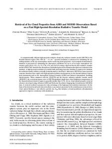
Fig. 15. Surface skin temperature; cloud optical depth, cloud height, and cloud particle size retrieved from IASI spectra taken on 29 April 2007.

face skin temperature; cloud optical depth, cloud height, and cloud particle size the altitude range from surface to 18 km. Again, the color ken on variation 29April 2007 represents the deviation of the temperature from the mean or the relative humidity. There is a lot of information on the retrieved three-dimensional atmospheric structures. For example, the upper atmosphere is warm and dry in the northwest side of the image, while the lower troposphere is cold with two moist layers moving horizontally. 4.2

Cloud and surface properties

The plots in Fig. 15 show retrieved surface skin temperature, cloud optical depth, cloud height, and cloud particle size from IASI spectra taken on 29 April 2007. The color scales are displayed in the figure. The white areas in the figure indicate the retrieval algorithm fails to converge due to multi-layer clouds or strong sun glint. Figure 16 shows the brightness temperature image of the IASI-integrated Imaging System (IIS). The IIS is an instrument that makes IR radiance Fig. 16. Brightness temperature measured by the high spatial resomeasurements in the spectral range from 10.3 to 12.5 µm. In lution IASI imager taken on 29 April 2007. Figure 16.2 byBrightness temperature measured by the high spatial resolution contrast to the IASI sounder which has 2 fields of view within a cell size of 45 km, 2007 the IIS has 64 by 64 pixels within the same cell size. Because of the high spatial resolution, the IASI imager brightness temperature provides good infortions from a collocated the IIS. For example, the altocumumation on cloud occurrences. Overall, the retrieved cloud lus clouds near West Virginia (near 38◦ latitude, −79◦ longifield from the IASI sounder compares well with the observatude) as seen by the imager are well captured by the physical

IASI ima

Figures 17 and 18 are plots of PCRTM retrieved surface emissivity spectra and


Atmos. Chem. Phys., 9, 9121–9142, 2009

the ARIES instrument for 19 April and 30 April.

The ARIES instrument did n

0.003) because the ocean surface is more uniform relative t 9134


ne: Surface emissivity retrieved from IASI spectra and taken on missivity over DOE-CART ARM site derived from the low flying Fig. 17. Blue line: Surface emissivity retrieved from IASI spectra and taken on 19 April 2007. Cyan line: land surface emissivity over DOE-CART ARM site derived from the low flying ARIES instrument.

e: Surface emissivity retrieved from IASI spectra and taken on missivity over DOE-CART ARM site derived from the low flying

Fig. 18. Blue line: Surface emissivity retrieved from IASI spectra over the Gulf of Mexico on 30 April 2007. Cyan line: surface emissivity derived from the low flying ARIES instrument.

retrieval algorithm. The retrieved cloud height is aroundfrom similar to those of surrounding areas, over again indicating e: Surface emissivity retrieved IASI spectra thethatGulf o 5 km with visible optical depth around 0.15. The cloud opthe physical retrieval system is capable of retrieving accurate tical depth is effective because the clouds infrom this region the may surface properties in theARIES presence of thin cirrus clouds. As rface emissivity derived low flying instrument not cover the whole IASI FOVs, The surface skin temperamentioned in Sect. 2.2, we have not performed any cloud retures under those altocumulus clouds are in the range of 284– 288 K, which is colder than the surrounding areas. This observation is consistent with the surface level air temperatures from radiosonde measurements in that area. The IASI measurements should see the surface in these area based on the imager data and on the retrieved small cloud optical depths. The cloud features near the Nebraska and Kansas state line (near 40◦ N latitude, 97◦ W longitude) seem to be high cirrus clouds (5–13 km) with a retrieved visible optical depths ranging from 0.1 to 0.2. The retrieved skin temperatures are

trieval validation due to the lack of quantitative truth data. The primary focus herein is on clear-air retrievals, and cloud parameter retrievals are included to show corresponding applicability of PCRTM methodology. Table 2 tabulates a quantitative comparison of the retrieved surface skin temperature from the IASI spectra with those measured by the UK Met Office’s Airborne Research Interferometer Evaluation System (ARIES) instrument for 19 April, 29 April, 30 April, and 4 May 2007. ARIES is an FTIR thermal emission radiometer with a 1 cm−1

mperature and moisture profiles e: Surface emissivity retrieved from IASI spectra over the Gulf o

face emissivity derived from the low flying ARIES instrument

wn that the IASI instrument is capable of providing very Atmos. Chem. Phys., 9, 9121–9142, 2009



9135

Table 2. Comparison of the PCRTM retrieved surface skin temperature from the IASI spectra with those measured by the ARIES instrument for 19 April, 29 April, 30 April, and 4 May 2007. Date

Location

Surface pressure (hPa)

Latitude/longitude (degree)

Satellite overpass time (UTC)

Skin temperature from ARIES (K)

Skin temperature from IASI (K)

19 Apr 2007 29 Apr 2007 30 Apr 2007 4 May 2007

Land Ocean Ocean Ocean

972.0 1021.7 1017.5 1009.9

88.5◦ W/26.5◦ N 90.5◦ W/26.9◦ N 88.5◦ W/26.5◦ N 92.0◦ W/27.5◦ N

03:35 15:50 15:29 15:46

284.7 297.8 298.6 297.4

284.8 297.6 298.1 297.1

wavenumber maximum spectral resolution over the range 600 to 3000 cm−1 wavenumbers. The method for deriving surface skin temperatures from the ARIES instrument is described by Newman et al. (2005). The agreement between the PCRTM retrieved and the ARIES measured skin temperatures is better than 0.5 K with a mean difference of 0.18 K. It should be noted that the footprint sizes of IASI and ARIES are different in the cross-track direction because the ARIES only makes NADIR measurements. Figures 17 and 18 are plots of PCRTM retrieved surface emissivity spectra and those measured by the ARIES instrument for 19 April and 30 April. The ARIES instrument did not measure surface emissivity on 29 April and 4 May. For the purpose of measuring surface emissivity and surface skin temperature, the ARIES instrument flew close to the Earth’s surface at very low altitudes. The ARIES instrument measured both upwelling and downwelling radiation and these radiances are then used to retrieve the surface emissivity and skin temperature simultaneously. There are many spectral regions where the ARIES does not provide surface emissivity retrievals because of the interferences from atmospheric CO2 , H2 O, and solar radiation. For the case of 19 April over the ARM-CART site, the IASI-retrieved emissivity agrees with the ARIES measured emissivity within 0.01 units. This agreement is good considering that the emissivity over the ARM-CART site is highly dependent on the percent coverage of vegetation within a specific area. The IASI covers a ground footprint of 12 km at nadir, while the ARIES instrument only covers tens of meters when flying near the surface. To minimize the difference due to spatial coverage, ARIES emissivity data is spatially averaged along the flight track during the IASI satellite overpass time. For 30 April 2007, the validation is during daytime and the IASI overpass took place over ocean in Gulf of Mexico. There is no ARIES emissivity retrieval at short wavelengths due to solar contaminations. The agreement between the ARIES measured and the IASI-retrieved emissivity is much better (within 0.003) because the ocean surface is more uniform relative to land.


4.3

Atmospheric temperature and moisture profiles

Section 4.1 has shown that the IASI instrument is capable of providing very detailed atmospheric temperature and moisture structures by using the PCRTM retrieval approach. In this section, we will perform case studies for 19 April, 29 April, 30 April, and 4 May 2007 during the JAIVEx campaign. The four cases were chosen based on coincidence of the aircraft under flights and the drop sondes with the IASI footprints. The location, the surface conditions and the time of satellite overpasses are listed in Table 2. At this stage of analysis, only clear FOVs are chosen for quantitative comparisons. Because the ARIES instrument only has NADIR views, the IASI scan angles are all close to NADIR views as well. We will show comparisons of the IASI-retrieved temperature and moisture profiles with those measured by the collocated dropsondes and the ECMWF model. We will analyze the retrieval quality by looking at the associated averaging kernels and the retrieval error covariance matrix. Figure 19 shows comparisons of the retrieved temperature and moisture vertical profiles with collocated dropsondes over the Oklahoma ARM CART site on 19 April 2007. The METOP-A satellite over-passed the ARM site around 03:35 UTC. Dropsondes were launched by the FAAM BAE146 aircraft, which flew a north-south track in the vicinity of the ARM-CART site near Lamont. Because the BAE-146 aircraft flew at an altitude of 12 km, ECMWF temperature and moisture profiles were used and interpolated to the location of the dropsondes for altitudes above the aircraft flying level. From the METOP-A AVHRR images, there were no clouds above at all levels during the time of the satellite overpass at 03:35 UTC. The climatology background was used for the first guess in the retrieval and they are plotted as black lines in Fig. 19. The IASI FOVs were selected based on the closeness to the BAE-146 flight path. The differences between the dropsonde and the retrieval are shown in the plots that are located in the second column of the figure. The averaging kernels and their integrated area for temperature and moisture profiles are shown in plots located on the right side of the first and second rows. The relative humidity and difference plots are also shown on the left side of the bottom row. The temperature and moisture error estimates Atmos. Chem. Phys., 9, 9121–9142, 2009

9136


Fig. 19. Top left panels: Temperature profiles of the dropsonde from the BAE-140 aircraft and the ECMWF model (blue line), the climatology first guess (black line), and the PCRTM retrieval (red line) for 19 April 2007. The difference plot is between the dropsonde and the retrieval. Top right panels: Temperature averaging kernels and the integrated area. Middle left panels: Moisture profiles of the dropsonde, the climatology first guess, and the PCRTM retrieval. The difference plot is between the radiosonde and the retrieval in mixing ratio unit. Middle right panels: Moisture averaging kernels in logarithm unit and the integrated area. Bottom left panels: Relative humidity profiles of the dropsonde, the climatology first guess, and the PCRTM retrieval. The difference plot is between the radiosonde and the retrieval. Bottom right panels: The temperature and moisture error estimates from the retrieval covariance matrix (Eq. 11).

op left panels: Temperature profiles of the dropsonde from the BAE-140 (blue line), the climatology first guess (black line), and the PCRTM retriev Thefromdifference plot between dropsonde the kernels retrieval. To the retrieval covariance matrixis are plotted on the bot- the plotted in logarithmic scale.and The averaging and the tom right portion of the figure. The agreement between the retrieval error estimates are also related to the logarithm of veraging kernels the integrated Middle left panels: Moisture IASI-retrieved and theand dropsonde/ECMWF temperature pro- area. water mixing ratio. The difference plot between the dropfiles are very good except near 90 hPa. The fine-scale error sonde and the retrieval is presented as mixing ratio in g/kg climatology first guess, and the PCRTM retrieval. The difference plot pattern is due to the null-space error which the retrieval syssince we cannot take a logarithm of the negative numbers. It tem has no sensitivity. Typically, theseratio fine-scale unit. error feais therefore difficult to see the retrieval errorMoisture in the difference avera the retrieval in mixing Middle right panels: tures are smaller than the half width of the corresponding avplot. In general, as the altitude increases the retrieval error kernel. It is evident fromBottom Fig. 19 that theleft integrated gets largerRelative and the averaginghumidity kernel gets broader. As men- of th nd theeraging integrated area. panels: profiles area for the temperature averaging kernels are all close to 1.0, tioned before, the integrated areas of averaging kernels for indicating the IASI measurement contains 100 percent The pressure levels less than 200 hPa areis smaller than one, indi-the rad t guess, andthatthe PCRTM retrieval. difference plot between information relative to climatology background. In order to cating that the climatology background contribute to the final om right panels: Thestructures, temperature and moisture error from the retr resolve those fine vertical other a priori informasolution. The retrieval errorsestimates are largest above 200 hPa which tion such as NWP forecast error covariance matrix and the is consistent with the retrieval error estimate and the averagn 11). associated forecast temperature profiles are needed. Because ing kernel area. For levels between the surface (972 hPa) and the water vapor mixing ratio changes by two orders of magnitude from surface to tropopause, the moisture profiles are

Atmos. Chem. Phys., 9, 9121–9142, 2009

800 hPa, the retrieved moisture profile also depends on the shape of the first guess. Fortunately for this day, the moisture


20 is the case study for 29 April, 2007. The aircraft flew a track run


9137

Fig. 20. Same as Fig. 19, except for 29 April 2007 over the Gulf of Mexico.

structure below 800 mbar is smooth and has similar shape as the a priori moisture profile. The retrieval performance is good for this case. The relative humidity plot shows more clearly how the retrieval is able to capture the large structure of the moisture vertical profile. For this case the relative humidity errors are less than 15 percent between the surface and 100 hPa. The agreement between the IASI-retrieved and the dropsonde/ECMWF temperature profiles are very good except near 90 hPa. The fine-scale error pattern is due to the null-space error which the retrieval system has no sensitivity. Typically, these fine-scale error features are smaller than the half width of the corresponding averaging kernel. It is evident from Fig. 19 that the integrated area for the temperature averaging kernels are all close to 1.0, indicating that the IASI measurement contains 100 percent information relative to climatology background. In order to resolve those fine vertical structures, other a priori information such as NWP forecast error covariance matrix and the associated forecast temperature profiles are needed. Because the water mixing ratio changes by two orders of magnitude from surface to tropopause, the moisture profiles are plotted in logarithmic scale. The averaging kernels and the retrieval error estimates

are also related to the logarithm of water mixing ratio. The difference plot between the dropsonde and the retrieval is presented as mixing ratio in g/kg since we cannot take a logarithm of the negative numbers. It is therefore difficult to see the retrieval error in the difference plot. In general, as the altitude increases the retrieval error gets larger and the averaging kernel gets broader. As mentioned before, the integrated areas of averaging kernels for pressure levels less than 200 hPa are smaller than one, indicating that the climatology background contributes to the final solution. The retrieval errors are largest above 200 hPa which is consistent with the retrieval error estimate and the averaging kernel area. For o (972 hPa) and 800 hPa, othe relevels between the surface trieved moisture profile also depends on the shape of the first guess. Fortunately for this case, the moisture structure below 800 mbar is smooth and has similar shape as the a priori moisture profile. The retrieval performance is good for this case. The relative humidity plot shows more clearly how the retrieval is able to capture the large structure of the moisture vertical profile. For this case the relative humidity errors are o less than 15 percent between the surface and 100 hPa.

me as Figure 19, except for 29 April 2007 over the Gulf of Mexico

21 is the case study for 30 April 2007.

The IASI overpass time is

measurements were made in a region near 88.5 W and 26.5 N over t

co.

Figure 22 is the case study for 4 May 2007.

The IASI over

The coincident measurements were made in a region near 92 W and 2 www.atmos-chem-phys.net/9/9121/2009/

co as well.

Atmos. Chem. Phys., 9, 9121–9142, 2009

The retrieval performance is very similar to that of

9138


Fig. 21. Same as Fig. 19, except for 30 April 2007 over the Gulf of Mexico.

Figure 20 is the case study for 29 April 2007. The aircraft flew a track running along the 90.5◦ W meridian over the ocean in the Gulf of Mexico. The IASI overpass time is at 15:50 UTC. For the region near 90.5◦ W and 26.9◦ N, the sky is free of clouds as identified in METOP AVHRR images. Our retrievals also show that the cloud optical depth is zero in this region (see Fig. 15). It can be seen that the temperature difference between the IASI retrieved and the dropsonde is large near the surface. The temperature averaging kernel for altitude below 900 hPa is about 0.7, indicating that the IASI spectrum does not provide 100 percent of the temperature information in this altitude range. This disparity is caused by the very small thermal contrast between the near surface air and the ocean surface. The dropsonde shows that the near surface air temperature is 296.64 K while the ocean surface temperature is 297.8 K. In addition to the low surface to air thermal contrast, the dropsonde measurement shows that the air temperature between 950 hPa to 1022 hPa is almost isothermal. Due to the small thermal contrast, any emissions and absorptions by the atmospheric CO2 and H2 O below 950 mbar will have very small signals, making it difficult to retrieve both temperature and moisture profile in this

narrow pressure range. The a priori profile (black line on the top right panel in Fig. 20) does not help the retrieval to get the isothermal structure since the background air temperature monotonically changes with pressure near the surface. For the case of 19 April, the near surface air temperature is about 4 K higher than the surface skin temperature and the air temperature increases with altitude; therefore the temperature averaging kernel near the surface is close to 1.0. Errors for the retrieved moisture profile for 29 April are larger than that of 19 April. The dropsonde moisture profile shows very fine vertical structures which are smaller than the half width of the moisture averaging kernels. The retrieval does capture the general shape of the moisture variation with the altitude. The errors are larger for pressure levels less than 200 mbar and for those levels between 800 mbar and the surface. This result is consistent with the averaging kernel information. For the altitude range between 500 mbar and 800 mbar, the errors seem to be larger than what is expected from the averaging kernels. This result may be due to too strong of regularization applied to the non-linear inversion process and will be studied further in the future.

me as Figure 19, except for 30 April 2007 over the Gulf of Mexico

Atmos. Chem. Phys., 9, 9121–9142, 2009



9139

Fig. 22. Same as Fig. 19, except for 4 May 2007 over the Gulf of Mexico.

Figure 21 is the case study for 30 April 2007. The IASI overpass time is at 15:29 UTC. The coincident measurements were made in a region near 88.5◦ W and 26.5◦ N over the ocean in the Gulf of Mexico. Figure 22 is the case study for 4 May 2007. The IASI overpass time is at 15:46 UTC. The coincident measurements were made in a region near 92◦ W and 27.5◦ N over the Gulf of Mexico as well. The retrieval performance is very similar to that of 29 April 2007. The temperature integrated areas of the averaging kernel for altitude below 900 hPa are smaller than 1.0. For both of these days, the thermal contrast between ocean surface and the near surface air temperature is still small (less than 1 K). The retrieved moisture profiles have captured the broad features while they missed all the fine details. For the cases of 29 April, 30 April, and 4 May, the measurements were made during the day-time and the retrievals do not use spectral region greater than 2000 cm−1 because handling solar radiation is not yet included in the retrieval process. When the solar zenith angle is less than 89 degrees, the magnitude of the solar component in spectral region 1800–2000 cm−1 typically varies from 0.1 K to 5 K in brightness temperature units, depending on the atmospheric conditions. We account for this

error source by adding an equivalent of 10 K error (brightness temperature calculated at 280 K) in this spectral region when we generate the Sy error covariance matrix during the inversion process. We will include the solar modeling and other trace gases in our future studies.

me as Figure 19, except for 4 May 2007 over the Gulf of Mexico

5

Summary and conclusions

5. Summary and superConclusions channels, we can retrieve atmospheric and surface We have demonstrated that by converting IASI spectra into properties efficiently from a PCRTM-based inversion algorithm. By performing the retrieval in EOF space, the algorithm is essentially using all the available IASI spectral information, but with a much smaller dimensions and faster speed. For a given state vector, the PCRTM model provides PC scores and associated Jacobian. The inversion approach is based on a maximum-likelihood method and uses the Levenberg-Marguardt algorithm for dealing with nonlinearity of the radiative transfer equation. We plan to run the PCRTM model in both the PC and the channel spaces so that we can quantify the pros and cons of the PC-based

ve demonstrated that by converting IASI spectra into super channels,

nd surface properties efficiently from a PCRTM-based inversion a

e retrieval in EOF space, the algorithm is Atmos. essentially using all the www.atmos-chem-phys.net/9/9121/2009/ Chem. Phys., 9, 9121–9142, 2009

mation, but with a much smaller dimensions and faster speed.

Fo

9140


methodology. In addition to atmospheric temperature and moisture profiles, cloud properties such as cloud optical depth, cloud particle size, cloud phase, and cloud top pressure are retrieved directly. Unlike the cloud-clearing algorithm, which relies on several FOVs in order to generate cloud-cleared radiances, the PCRTM-based retrieval algorithm is performed on a single IASI field of view (FOV) and can be done for both clear and cloudy FOVs. Currently, we have no quantitative validation of the retrieved cloud parameters and we plan to validate our cloud retrieval methodology by collocating IASI data with those from A-train data in a future study. We have applied the super channel retrieval algorithm to IASI spectra taken during the JAIVEx field campaign in the spring of 2007. The retrieval algorithm is capable of fitting IASI radiances to within instrument noise level at most frequency ranges. Currently, we set the “noise-level” as the original IASI instrument noise specifications. Although the radiance residuals in many spectral regions (most noticeably in band 3) are much less than the native IASI noise, we decided not to fit the radiance spectrum to the PC-filtered noise level at this stage because we have not accounted for many error sources such as uncertainty in spectroscopy and errors caused by trace gases that are not currently retrieved in the inversion process. Due to the high information content of the IASI instrument, three-dimensional atmospheric structure can be effectively retrieved using the PCRTM-based retrieval algorithm. The retrieved cloud features compare well with the collocated IIS data. The retrieved surface emissivity data and surface skin temperatures compare well with the measurements from the ARIES instrument. Quantitative comparisons of the retrieved atmospheric temperature and moisture profiles have been compared with airborne dropsonde measurements from the BAE-146 aircraft for 19 April, 29 April, 30 April, and 4 May. Averaging kernels corresponding to those retrievals have been plotted to reveal the insight of the vertical resolution of the retrieved temperature and moisture profiles. The integrated areas and the peak locations of the averaging kernels provide the information content for each atmospheric level. In general, the retrieval errors are consistent with the information content analysis and the error estimate from the retrieval system. Although, ozone and CO are already retrieved in our current algorithm, we will validate the products in our future work. We plan to further study the impact of a priori information and the effect of not retrieving other trace gases on accuracy of temperature and moisture retrievals. Acknowledgements. The authors would like to thank for the contributions from the NASA Langley Research Center, the EUMETSAT, the UK Met Office, and the Space Science and Engineering Center of the University of Wisconsin-Madison. Thanks to NCAR team (especially L. Emmons) for MOZART CO and other trace gas profiles. This work is supported by funds from the NASA Headquarters and the NPOESS Integrated Program Office (IPO). The FAAM is jointly funded by the UK Met Office and the

Atmos. Chem. Phys., 9, 9121–9142, 2009

Natural Environment Research Council. IASI has been developed and built under the responsibility of the Centre National d’Etudes Spatiales (CNES, France). It is flown onboard the Metop satellites as part of the EUMETSAT Polar System. The IASI L1 data are received through the EUMETCast near real time data distribution service. We thank Ping Yang and his group for providing the cloud properties used in this study. We would also like to thank the anonymous reviewers for their comments and suggestions. Edited by: T. Wagner

References Aoki, T.: Channel Compression of Trace Gas Remote Sounder by Expanding the Weighting Function with Empirical Orthogonal Functions, J. Meteorol. Soc. Jpn., 82, 1081–1093, 2004. Aoki, T.: Channel Compression of High Resolution Infrared Spectra with Using Hypothetical Channel System, J. Meteorol. Soc. Jpn., 83, 41–55, 2005. Aumann, H. H., Chahine, M. T., Gautier, C., Goldberg, M. D., Kalnay, E., McMillin, L. M., Revercomb, H., Rosenkranz, P. W., Smith, W. L., Staelin, D. H., Strow, L. L., and Sussind, J.: AIRS/AMSU/HSB on Aqua Mission: Design, Science objectives, data products, and processing system, IEEE Trans. Geosci. Rem. Sens., 41, 253–264, 2003. Barnet, C. D., Blaisdell, J. M., and Susskind, J.: Practical Methods for Rapid and Accurate Computation of Interferometric Spectra for Remote Sensing Applications, IEEE Trans. Geosci. Rem. Sens., 38, 169–183, 2000. Blumstein, D., Chalon, G., Carlier, T., Buil, C., Hebert, P., Maciaszek, T., Ponce, G., and Phulpin, T.:: IASI instrument: technical overview and measured performances, SPIE Proc., 5543, 196–207, 2004. Baum, B. A., Yang, P., Nasiri, S., Heidinger, A. K., Heymsfield, A. J., and Li, J.: Bulk Scattering Properties for the Remote Sensing of Ice Clouds. III: High resolution spectral models from 100 to 3250 cm−1 , J. Appl. Meteor. Clim., 46, 423–434, 2007. Chahine, M. T.: Remote sounding cloudy atmospheres. I. The Single Cloud Layer, J. Atmos. Sci., 31, 233–243, 1974. Chahine, M. T.: Remote sounding cloudy atmospheres. II. Multiple Cloud Formations, J. Atmos. Sci., 34, 744–757, 1977. Chahine, M. T., Aumann, H., Goldberg, M., McMillin, L., Rosenkranz, P., Staelin, D., Strow, L., Susskind, J., and Gunson, M.: AIRS Level 2 Algorithm Theoretical Basis Document Version 2.2, JPL D-17006, 2001. Clough, S. A. and Iacono, M. J.: Line-by-line calculation of atmospheric fluxes and cooling rates: 2. Application to carbon dioxide, ozone, methane, nitrous oxide and the halocarbons, J. Geophys. Res., 100, 16579–16593, 1995. Collard, A.: Selection of IASI Channels for Use in Numerical Weather Prediction, Q. J. Roy. Meteorol. Soc., 629, 1977–1991, 2007. Collard, A. and McNally, T.: Operational Assimilation of IASI radiances at ECMWF, Joint Center for Satellite Data Assimilation Quarterly, 22, 2–3, 2008. Crevoisier, C., Chedin, A., and Scott, N.: AIRS channel selection for CO2 and other trace-gas retrievals, Q. J. Roy. Meteorol. Soc., 129, 2719–2740, 2003.


X. Liu et al.: Retrieval of atmospheric profiles and cloud properties Edwards, D. P. and Francis, G. L.: Improvements to the correlated-k radiative transfer method: Application to satellite infrared sounding, J. Geophys. Res., 105(D14), 18135–18156, 2000. Eyre, J. R.: Inversion of cloudy satellite sounding radiances by nonlinear optimal interpolation. I: Theory and simluation for TOVS, Q. J. Roy. Meteorol. Soc., 115, 1001–1026, 1989a. Eyre, J. R.: Inversion of cloudy satellite sounding radiances by nonlinear optimal estimation. II: Application to TOVS data, Q. J. Roy. Meteorol. Soc., 115, 1027–1037, 1989b. Fourrié, N. and Thépaut, J.-N.: Validation of the NESDIS near real time AIRS channel selection. ECMWF Tech. Memo. 390, European Center for Medium Range Weather Forecasts, Reading, UK, 2002. Fourrié, N. and Thépaut, J.-N.: Evaluation of the AIRS near-realtime channel selection for application to numerical weather prediction, Q. J. Roy. Meteorol. Soc., 129, 2425–2439, 2003. Goldberg, M. D., Qu, Y., McMillin, L. M., Wolf, W., Zhou, L., and Divakarla, M.: AIRS near real-time products and algorithms in support of operational numerical weather prediction, IEEE Trans. Geosci. Rem. Sens., 41, 379–389, 2003. Huang, H.-L. and Antonelli, P.: Application of principal component analysis to high-resolution infrared measurement compression and retrieval, J. Appl. Meteorol., 40, 265–388, 2001. Huang, H.-L., Yang, P., Wei, H., Baum, B. A., Hu, Y. X., Atonelli, P., et al.: Inference of ice cloud properties from high-spectral resolution infrared observations, IEEE Trans. Geosci. Rem. Sens., 42, 842–852, 2004. Niu, J. G., Ping, Y., Huang, H.-L., Davies, J. E., Li, J., Baumc, B. A., and Hu, Y. X.: A fast infrared radiative transfer model for overlapping clouds, J. Quant. Spectros. Radiat. Transfer, 103, 447–459, 2007. Klaes, K. D., Cohen, M., Buhler, Y., Schluessel, P., Munro, P., Luntama, J.-P., Von Engeln, A., Clerigh, E. O., Bonekamp, H., Ackernmann, J., and Schmetz, J.: An introduction to the EUMETSAT Polar System, B. Am. Meteorol. Soc., 88, 1085–1096, 2007. Kinnison, D. E., Brasseur, G. P., Walters, S., Garcia, R. R., Marsh, D. R., and Sassi, F., Harvey, V. L., Randall, C. E., Emmons, L., Lamarque, J. F., Hess, P., Orlando, J. J., Tie, X. X., Randel, W., Pan, L. L., Gettelman, A., Granier, C., Diehl, T., Niemeier, U., and Simmons, A. J.: Sensitivity of chemical tracers to meteorological parameters in the MOZART-3 chemical transport model, J. Geophys. Res., 112, D20302, doi:10.1029/2006JD007879, 2007. Le Marshall, J., Jung, J., Derber, J., Chahine, M., Treadon, R., Lord, S., Goldberg, M., Wolf, W., Liu, H. C., Joiner, J., Woollen, J., Todling, R., van Delst, P., and Tahara, Y.: Improving Global Analysis and Forecasting with AIRS, B. Am. Meteorol. Soc., 87, 747–750, 2006. Le Marshall, J., Jung, J., Derber, J., Treadon, R., Lord, S., Goldberg, M., Wolf, W., Liu, H. C., Joiner, J., Woollen, J., and Todling, R.: AIRS hyperspectral data improves southern hemisphere forecasts, Aust. Meteor. Mag., 54, 57–60, 2005a. Le Marshall, J., Jung, J., Derber, J., Treadon, R., Lord, S., Goldberg, M., Wolf, W., Liu, H. C., Joiner, J., Woollen, J., and Todling, R.: Impact of Atmospheric InfraRed Sounder Observations on Weather Forecasts, EOS, 86, 109, 115, 116, 15 March 2005b. Li, J., Liu, C. Y., Huang, H.-L., Schmit, T. J., Menzel, W. P., and Gurka, J.: Optimal cloud-clearing for AIRS radiances using MODIS, IEEE Trans. Geosci. Rem. Sens., 43, 1266–1278,


9141

2005. Liu, X. W., Smith, L., Zhou, D. K., and Larar, A.: A principal component-based radiative transfer forward model (PCRTM) for hyperspectral instruments, Proc. SPIE Int. Soc. Opt. Eng., 5655, 96–105, 2005. Liu, X., Zhou, D. K., Larar, A., Smith, W. L., and Mango, S. A.: Case Study a New Radiative Transfer Model and Retrieval Algorithm using EAQUATE Data, Q. J. Roy. Meteorol. Soc., 133, 243–256, 2007. Liu, X., Moncet, J.-L., Zhou, D. K., and Smith, W. L.: A Fast and Accurate Forward Model for NAST-I Instrument, in: Fourier Transform Spectroscopy and Optical Remote Sensing of Atmosphere, 2003 Technical Digest Series OSA (Optical Society of America, Washington, D.C., 2003), p. 16, 2003. Liu, X., Smith, W. L., Zhou, D. K., and Larar, A.: Principal Component-based Radiative Transfer Forward Model (PCRTM) For Hyperspectral Sensors, Theoretical Concept, Appl. Optics, 45, 201–209, 2006. Marquardt, D.:: An Algorithm for Least-Squares Estimation of Nonlinear Parameters, SIAM J. Appl. Math., 11, 431–441, 1963. Masuda, K., Takashima, T., and Takayama, Y.: Emissivity of pure and sea waters for the model sea surface in the infrared window regions, Rem. Sens. Environm., 24, 319–329, 1988. Matricardi, M.: RTIASI-4, a new version of the ECMWF fast radiative transfer model for infrared atmospheric sounding interferometer, ECMWF Tech. Memo., 425, 63 pp., 2003. Matricardi, M. and Saunders, R. W.: A fast radiative transfer model for simulation of IASI radiances, Appl. Optics, 38, 5679–5691, 1999. McMillin, L. M., Goldberg, M. D., Ding, H., Susskind, J., and Barnet, C. D.: A forward calculation for interferometers: method and validation, Appl. Optics, 37, 3059–3068, 1997. McMillin, L. M., Crone, L. J., and Kleespies, T. J.: Atmospheric transmittance of an absorbing gas, 5, Improvements to the OPTRAN approach, Appl. Optics, 34, 8396–8399, 1995. McMillin, L. M.: Super Channels for AIRS Retrievals, AMS 13th Conference on Satellite Meteorology and Oceanography, 19– 23 September 2004, Norfolk, VA, http://ams.confex.com/ams/ pdfpapers/78955.pdf, 2004. Menzel, W., Smith T., and Stewart, T. R.: Improved cloud motion vector and altitude assignment using VAS, J. Appl. Meteorol., 22, 377–384, 1983. Moncet, J.-L., Liu, X., Helene, R., Snell, H., Zaccheo, S., Lynch, R., Eluszkiewicz, J., He, Y., Uymin, G., Lietzke, C., Hegarty, J., Boukabara, S., Lipton, A., and Pickle, J.: Algorithm Theoretical Basis Document (ATBD) for the Cross Track Infrared Sounder (CrIS) Environmental Data Records (EDR), V1.2.3, AER Document Released to ITT and Integrated Program Office, 2001. Moncet, J. L. and Clough, S. A.: Accelerated monochromatic radiative transfer for scattering atmospheres: application of a new model tospectral radiance observations, J. Geophys. Res., 102, 853–866, 1997. Newman, S. M., Smith, J. A., Glew, M. D., Rogers, S. M., and Taylor, J. P.: Temperature and salinity dependence of sea surface emissivity in the thermal infrared, Q. J. Roy. Meteorol. Soc., 131, 2539–2557, 2005. Pagano, T. S., Aumann, H. H., Hagan, D. E., and Overoye, K.: Prelaunch and in-flight radiometric calibration of the Atmospheric Infrared Sounder (AIRS), IEEE Trans. Geosci. Rem.

Atmos. Chem. Phys., 9, 9121–9142, 2009

9142


Sens., 41, 265–273, 2003. Press, W. H., Teukolsky, S. A., Vetterling, W. T., and Flannery, B. P.: Numerical Recipes (second edition), Cambridge Press, 1992. Prunet, P., Thépaut, J.-N., and Cassé, V.: The information content of clear sky IASI radiances and their potential for numerical weather prediction, Q. J. Roy. Meteorol. Soc., 124, 211–241, 1998. Rabier, F., Fourrié, N., Chafa¨ı, D., and Prunet, P.: Channel selection methods for Infrared Atmospheric Sounding Interferometer radiances, Q. J. Roy. Meteorol. Soc., 128, 1011–1027, 2002. Rodgers, C. D.: Inverse Methods for Atmospheric Sounding – Theory and Practice, World Scientific, Singapore, pp 238, 2002. Rodgers, C. D.: Retrieval of atmospheric temperature and composition from remote measurements of thermal radiation, Rev. Geophys. Space Phys., 14, 609–624, 1976. Salisbury, J. W. and D’Aria, D. M.: Emissivity of terrestrial material in the 8–14 µm atmospheric window, Rem. Sens. Environ., 42, 83–106, 1992. Saunders, R., Matricardi, M., and Brunel, P.: An improved fast radiative transfer model for assimilation of satellite radiance observations, Q. J. Roy. Meteorol. Soc., 125, 1407–1425, 1999. Saunders, R., Rayer, P., Brunel, P., von Engeln, A., Bormann, N., Strow, L., Hannon, S., Heilliette, S., Liu, X., Miskolczi, F., Han, Y., Masiello, G., Moncet, J.-L., Uymin, G., Sherlock, V., and Turner, D. S.: A comparison of radiative transfer models for simulating AIRS radiances, J. Geophys. Res., 112, D01S90, doi:10.1029/2006JD007088, 2007. Schluessel, P.: Super-Channel Selection for IASI Retrievals, ITSC XIV Proceedings, Beijing, China, 25–31 May 2005, (http://cimss.ssec.wisc.edu/itwg/itsc/itsc14/proceedings/ 11 2 Schluessel.pdf), 2005. Schluessel, P., Hultberg, T. H., Phillips, P. L., August, T., and Calbet, X.: The operational IASI Level 2 processor, Adv. Space Res., 36, 982–988, 2005. Segelstein, D. J.: The complex refractive index of water, Master’s thesis, University of Missouri-Kansas City, 1981. Smith, W. L.: An improved method for calculating tropospheric temperature and moisture from satellite radiometer measurements, Mon. Weather Rev., 96, 387–396, 1968. Smith, W. L., Huang, H. L., and Jenney, J. A.: An advanced sounder cloud contamination study, J. Appl. Meteor., 35, 1249–1255, 1996. Smith, W. L.: An improved method for calculating tropospheric temperature and moisture from satellite radiometer measurements, Mon. Weather Rev., 96, 387–396, 1968. Stamnes, K., Tsay, S.-C., Wiscombe, W., and Jayaweera, K.: Numerically stable algorithm for discrete-ordinate-method radiative transfer in multiple scattering and emitting media, Appl. Optics, 27, 2502–2509, 1988.

Atmos. Chem. Phys., 9, 9121–9142, 2009

Strow, L. L., Hannon, S. E., De Souza-Machado, S., Motteler, H. E., and Tobin, D.: An overview of the AIRS radiative transfer model, IEEE Trans. Geosci. Rem. Sens., 41, 303–313, 2003. Strow, L. L., Hannon, S. E., De-Souza Machado, S., Motteler, H. E., and Tobin, D. C.: Validation of the Atmospheric Infrared Sounder radiative transfer algorithm, J. Geophys. Res., 111, D09S06, doi:10.1029/2005JD006146, 2006. Susskind, J., Barnet, C., Blaisdell, J., Iredell, L., Keita, F., Kouvaris, L., Molnar, G., and Chahine, M.: Accuracy of geophysical parameters derived from Atmospheric Infrared Sounder/Advanced Microwave Sounding Unit as a function of fractional cloud cover, J. Geophys. Res., 111, D09S17, doi:10.1029/2005JD006272, 2006. Susskind, J., Barnet, C. D., and Blaisdell, J. M.: Retrieval of atmospheric and surface parameters from AIRS/AMSU/HSB data in presence of clouds, IEEE Trans. Geosci. Rem. Sens., 41, 390– 409, 2003. Warren, S. G.: Optical constants of ice from the ultraviolet to the microwave, Appl. Optics, 23, 1206–1225, 1984. Wei, H., Yang, P., Li, J., Baum, B. A., Huang, H., Platnick, S., et al.: Retrieval of semitransparent ice cloud optical thickness from atmospheric infrared sounder (AIRS) measurements, IEEE Trans. Geosci. Rem. Sens., 42, 2254–2267, 2007. Wu, X. Q. and Smith, W. L.: Emissivity of rough sea surface for 8–13 microns: Modeling and verification, Appl. Optics, 36(12), 2609–2619, 1997. Yang, P., Gao, B. C., Baum, B. A., Hu, Y., Wiscombe, W. J., Tsay, S.-C., Winker, D. M., and Nasiri, S. L.: Radiative Properties of cirrus clouds in the infrared (8–13 µm) spectral region, J. Quant. Spectros. Radiat. Transfer, 70, 473–504, 2001. Zhang, Z., Yang, P., Kattawar, G., Huang, H.-L., Greenwald, T., Li, J., Baum, B. A., Zhou, D. K., and Hu, Y.: A fast infrared radiative transfer model based on the adding–doubling method for hyperspectral remote-sensing applications, J. Quant. Spectros. Radiat. Transfer, 105, 243–263, doi:10.1016/j.jqrt.2007.01.009, 2007. Zhou, D. K., Smith Sr., W. L., Liu, X., Larar, A. M., Mango, S. A., and Huang, H.-L.: Physically retrieving cloud and thermodynamic parameters from ultraspectral IR measurements, J. Atmos. Sci., 64, 969–982, 2007. Zhou, D. K., Smith, W. L., Liu, X., Larar, A. M., Huang, H.-L. A., Li, J., McGill, M. J., and Mango, S. A.: Thermodynamic and cloud parameters retrieval using infrared spectral data, Geophys. Res. Lett., 32, L15805, doi:10.1029/2005GL023211, 2005. Zhou, D. K., Smith, W. L., Larar, A. M., Liu, X., Taylor, J. P., Schlüssel, P., Strow, L. L., and Mango, S. A.: All weather IASI single field-of-view retrievals: case study – validation with JAIVEx data, Atmos. Chem. Phys., 9, 2241–2255, 2009, http://www.atmos-chem-phys.net/9/2241/2009/.


Retrieval of atmospheric profiles and cloud properties ... - CiteSeerX

Retrieval of atmospheric profiles and cloud properties ... - CiteSeerX

Suggest Documents

Retrieval of atmospheric profiles and cloud ... - Atmos. Chem. Phys

Retrieval of temperature profiles and cloud ... - Meeting Organizer

5.3 RETRIEVAL OF BOUNDARY LAYER CLOUD PROPERTIES ...

Retrieval of Ice Cloud Properties from AIRS and ... - MODIS Atmosphere

Thermodynamic and cloud parameter retrieval using ... - CiteSeerX

Satellite-pointing retrieval from atmospheric limb ... - CiteSeerX

ARM Cloud Retrieval Ensemble Data Set (ACRED) - Atmospheric ...

Hygroscopic properties of atmospheric aerosol particles ... - CiteSeerX

Retrieval of ice cloud properties using an ... - Wiley Online Library

Retrieval of Cirrus Cloud Properties From the ... - IEEE Xplore

Retrieval of ice cloud properties using an ... - Wiley Online Library

Direct Retrieval of Line-of-Sight Atmospheric Structure ... - CiteSeerX

Retrieval and validation of Cloud Motion Vectors (CMV) - CiteSeerX

Retrieval of cloud pressure and oceanic chlorophyll ... - CiteSeerX

Retrieval of the scattering and microphysical properties of ... - CiteSeerX

On retrieval of lidar extinction profiles using Two-Stream ... - CiteSeerX

Unsupervised Retrieval of Attack Profiles in Collaborative ... - CiteSeerX

Spectral Retrieval of Latent Heating Profiles from TRMM ... - CiteSeerX

density profiles, escape flux and atmospheric stability

User-profiles for Information Retrieval

Atmospheric Temperature, Moisture and Trace Gas Retrieval ...

Cloud Optical Property Retrieval

P1.19 Retrieval of Cloud Liquid Water Content Profiles with Radar and ...

Hyperspectral remote sensing of atmospheric profiles