REVEALING THE DYNAMIC CORRELATION BETWEEN NEURAL AND MUSCULAR SIGNALS USING TIMEDEPENDENT GRANGER CAUSALITY ANALYSIS S.Y. Wang1, Y. Chen2, M. Ding2, J. Feng3, J.F. Stein1, T.Z. Aziz4, X. Liu5* 1 University Laboratory of Physiology, University of Oxford, UK; 2 Department of Biomedical Engineering, University of Florida, USA, 3 Centre for Scientific Computing, University of Warwick, UK; 4 Nuffield Department of Surgery, University of Oxford, UK; 5 Division of Neuroscience and Mental Health, Imperial College London, UK. *Corresponding Author: Email:
[email protected]
Keywords: causality, coherence, autoregressive model, functional coupling between two oscillatory signals is the subthalamic nucleus, electromyogram
muscle,
local
field
potential,
Abstract Functional correlation between oscillatory neural and muscular signals during tremor can be revealed by Fouriertransform-based coherence estimation. The coherence value in a defined frequency range reveals the interaction strength between the two signals. However, coherence estimation does not provide directional information, preventing the further dissection of the relationship between the two interacting signals. We have therefore investigated functional correlations between the subthalamic nucleus (STN) and muscle in Parkinsonian tremor using adaptive Granger autoregressive modelling. During intermittent resting tremor we analysed the inter-dependence of local field potentials (LFPs) recorded from the STN and surface electromyograms (EMGs) recorded from the contralateral forearm muscles. We compared the Granger causality with coherence estimation, an adaptive Granger causality based on autoregressive modelling with a running window was used to reveal the time-dependent causal influences between the LFP and EMG signals. Our results showed that during persistent tremor, there was a directional causality predominantly from EMGs to LFPs corresponding to the significant coherence between LFPs and EMGs at the tremor frequency; and over episodes of transient resting tremor, the inter-dependence between EMGs and LFPs was bi-directional and alternatively varied with time. We conclude that the functional correlation between the STN and muscle is dynamic, bi-directional, and dependent on the tremor status.
1 Introduction Analysis of functional coupling between muscular activity and simultaneously recorded oscillatory neural activity at different levels of the motor system has provided important insights into neural control of movement. It has led not only to a better understanding of the pathophysiological mechanisms of movement disorders but also to better localization of targets for deep brain stimulation (DBS) (for a review, see [10]) One widely used method of estimating the
magnitude squared coherence (MSC). The MSC is a normalized cross-spectral density function, and measures the strength of association and relative linearity between two stationary processes on a scale from zero to one [14]. The coherence value indicates the strength of the coupling in the frequency domain. However, the coherence function is unable to distinguish between a closed- and an open- loop system. Similar significant coherence estimation may appear in both systems with and without feedback. Thus it does not help to elucidate any causal relationships within the system. Therefore, to fully understand information processing at different levels of the motor system, directional analysis to reveal causal influence between signals is essential. Granger causality analysis [6] has proved useful in this kind of situation [1,8,9]. In a recent study, Granger analysis was performed for all pairwise combinations of oscillatory field potential activity in the beta (14–30 Hz) frequency range among sensorimotor cortical recording sites during a GO/NOGO visual pattern discrimination task in monkeys [2]. In the present study, we performed windowed Granger causality analysis to quantify the time-dependent coupling between two simultaneously recorded neural and muscular signals. The electromyograms (EMGs) recorded from muscle surfaces can be considered a stochastic (zero–mean) process resulting from the electrical activity of activated muscle fibres. In contrast to oscillatory neural signals, the physiological output from the central motor system is usually encoded in the ‘envelope’ of the compound EMG signal rather than in the individual action potentials of muscle fibres. We pre-processed the EMG signals, validated our autoregressive (AR) models and investigated influence of noise and the time-dependent Causality with running window. We then used Granger causality analysis to reveal any causal correlation between local field potentials (LFPs) of the subthalamic nucleus (STN) and the EMGs of forearm muscles in patients with Parkinsonian resting tremor.
2 Methods 2.1. Description of coherence and Granger causality Autoregressive representations of wide-sense stationary time series x1(t) and x2(t) are
∞
x1 (t ) = ∑ a1 ( k ) x1 (t − k ) + u1 (t )
(1)
x2 (t ) = ∑ a 2 (k ) x2 (t − k ) + u 2 (t )
(2)
k =1 ∞ k =1
where the parameters a1(k) and a2(k) are the model coefficients, u1(t) and u2(t) are the prediction error when x1(t) and x2(t) are predicted from its own past respectively. The variance of u1(t) and u2(t) are Σ1 and Σ2. The linear dependence between these two signals can be expressed as a bivariate AR model ∞
(3)
x 2 (t ) = ∑ a 21 (k ) x1 (t − k ) + ∑ a 22 (k ) x 2 (t − k ) + v 2 (t )
(4)
k =1 ∞
k =1 ∞
k =1
k =1
S12 ( f )
2
S11 ( f ) S 22 ( f )
The measure of Granger causality from x2(t) and x1(t) is defined as Fx2→x1=ln(Σ1/Σ11). Fx2→x1 is nonnegative. If Σ1=Σ11, Fx2→x1=0 which indicates x2(t) does not cause x1(t) [5]. The measure of Fx2→x1 is invariant when x2(t) and x1(t) are rescaled or pre-multiplied by different invertible lag operators. Symmetrically, the measure of causality from x1(t) to x2(t) is defined as Fx1→x2=ln(Σ2/Σ22). The causality Fx2→x1 measures the reduction in the total variance of predictive errors of x1(t) when past x2(t) is added for prediction and used as their causality measure Fx2→x1. The percentage reduction of the variance R 2 = 1 − e− F suggests the degree of x1(t) relating to the history of x2(t).
∞
x1 (t ) = ∑ a11 ( k ) x1 (t − k ) + ∑ a12 (k ) x 2 (t − k ) + v1 (t )
γ xy2 ( f ) =
x2 → x1
where the parameters aij(k) are the model coefficients, v1(t) is the prediction error when x1(t) is predicted from its own past and past of x2(t), and similarly for v2(t). The above equations can be expressed in the matrix form as X (t ) = [ x1 (t ), x 2 (t )] T ,
⎡ a (k ) a12 (k ) ⎤ A(k ) = − ⎢ 11 and V (t ) = [v1 (t ), v 2 (t )] ⎥ ⎣a21 (k ) a22 (k )⎦ (subscript T stands for transpose), then
Fx2→x1 can be decomposed in frequency domain [5] as Fx1 → x2 ( f ) = ln
S 22 ( f ) * S 22 ( f ) − H 21 ( f )( Σ11 − Σ12 / Σ 22 ) H 21 (f) 2
T
and Fx2 → x1 ( f ) = ln
S11 ( f ) S11 ( f ) − H 12 ( f )( Σ 22 − Σ12 / Σ11 ) H 12* ( f ) 2
.
∞
X (t ) = −∑ A(k ) X (t − k ) + V (t )
(5)
k =1
The normalised causality measures are given as
Let A(0)=I, the identity matrix, equation (5) can be re-written ∞
as
∑ A(k ) X (t − k ) = V (t )
(6)
k =0
The spectral relationship of equation (6) can be written as
Rx22 → x1 ( f ) = 1 − e
− Fx
Rx21→x2 ( f ) = 1 − e
− Fx
2 → x1
1 → x2
(f)
(f)
(8) (9)
in the scale of 0 to 1.
A ( f ) X ( f ) = V ( f ) , in which
2.2. Signal recording and pre-processing
X ( f ) = A −1 ( f ) V ( f ) = H ( f ) V ( f ) ∞
−ik 2πf and A ( f ) = ∑ A ( k )e
(7)
k =0
The power spectral matrix of the signals is then given by S(f)= X(f)X*(f)= H(f)V(f)V*(f)H*(f)=H(f)ΣH*(f) ⎡ Σ11 where * stands for conjugate transpose. Σ = ⎢ ⎣ Σ 21
co-variance
matrix
of
v1(t)
and
v2(t)
Σ12 ⎤ is the Σ 22 ⎥⎦
and,
and
⎡ S ( f ) S12 ( f ) ⎤ S( f ) = ⎢ 11 ⎥ is the spectral matrix of x1(t) and ⎣S 21 ( f ) S 22 ( f )⎦
x2(t) and, where S11(f) and S22(f) are the auto-spectra of x1(t) and x2(t) and S12(f) and S21(f) are their cross-spectra. The MSC is defined as the normalized cross-spectral density by the autospectral densities [3,7]:
The study was approved by the local research ethics committee, and informed consent was obtained from each of five patients with resting tremor due to PD who underwent chronic stimulation in both STNs at the Radcliffe Infirmary, Oxford. Detailed surgical procedures and target localisation have been described previously [11]. LFPs were recorded with a bipolar configuration from the adjacent 4 contacts of each macroelectrode (0-1, 1-2, 2-3) with a common electrode placed on the surface of the mastoid. Localisation of the electrode was confirmed by postoperative magnetic resonance imaging. EMGs were recorded using surface electrodes placed in a tripolar configuration over the tremulous forearm extensor and flexors. Signals were amplified using isolated CED 1902 amplifiers (×10,000 for LFPs and ×1,000 for EMGs), filtered at 0.5-500Hz and digitised using CED 1401 mark II at 4000Hz using Spike2 (Cambridge Electronic Design, Cambridge, UK).
2.3. Selection and validation of AR models The optimal model order is determined according to the criteria which are usually based on the statistics constructed from prediction errors. Akaike’s Information Criterion (AIC)
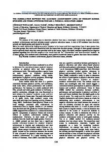
3. Results 3.1. Pre-processing The surface EMGs were compound signals of multi-unit activity and had a broad frequency distribution. The tremor related activity, , presented as synchronised rhythmic bursts at 5Hz (Fig.1A) independent of the individual muscle fibre action potentials. The tremor bursts were isolated firstly by performing full-wave rectification (Fig. 1B) and further by extracting the envelope following low-pass filtering the rectified EMGs and down-sampling at 100Hz (Fig. 1C). Similar filtering and down-sampling were performed on the LFP signals.
We determined the optimal model order for recordings from each patient according to AIC and validated the model with the prediction ratio and autocorrelation of the prediction error.
2
0.24
0 -40
0.12 0.00 0
PSD(µV /Hz)
2
40 20 0
100 200 300 400 500 Frequency (Hz)
6 4 2 0 0
10 20 Frequency (Hz)
30
10 20 Frequency (Hz)
30
B PSD(µV /Hz)
20
2
The model can be validated by assessing the quality of the model fitness of the prediction ratio [12] which measures how much the model can explain the variance of the signal and the percentage of the variance contributed from the model in the total variance. This provides objective criteria on whether the model is capable of characterise the system dynamics. For perfect fitness, the prediction error is zero. If the model is correct and the true parameter values are estimated properly, the prediction error would be white noise. If the autocorrelation function shows pronounced patterns, such as the ripples or slow decline at low lags, it suggests model inadequacy.
1s
40
A EMGs(µV)
matrix assuming an ith order model, N is the number of data points and L is the number of variables. AIC should be computed only for a maximum value of i of 3 N / L in order to produce reliable results. The optimal model order corresponds to the minimum of AIC(i).
EMGs(µV)
ˆ is the estimate of the prediction error covariance where Σ i
EMGs(µV)
ˆ )+2L2i is the most commonly used one, AIC(i)=Nlog(det( Σ i
PSD(µV /Hz)
The EMGs were high-pass filtered above 15 Hz using wavelet transforms to remove the motion artefacts. Then the EMGs were rectified in order to extract the EMG envelope signal. Both rectified EMGs and LFPs were low-pass filtered (corner frequency: 30Hz). Then both signals were down-sampled to 100Hz and detrended for further coherence and causality analysis. All signal processing was performed using MATLAB (Version 6.5, MathWorks Inc., Natick, Ma., USA).
10 0
6 4 2 0 0
C Figure 1. Extracting the envelop of the tremor bursts in the surface EMG signal. A: EMG signal of multi-unit activity with a broad frequency distribution; B: full-wave rectification to enhance the tremor rhythmic bursts; and C: extracting the envelop of the tremor bursts by low-pass filtering and down-sampling. 3.2. Selection and validation of AR model
2.4. Short-window coherence and causality analysis
In the present study, we selected a 3-second window as it is longer than three times of the model order, and it gives adequate time and frequency resolutions for observing the resting tremor of predominant 4.8Hz within a band of 0 – 30Hz with events of its onset and cessation occurring over a few seconds.
B
-1.4
0
-1.6
-2 20 10
-1.8 AIC
A
LFPs(µV)
The optimal model order of the bivariate AR model of each pair of LFP and EMG signals was determined from the AIC curve (Fig. 2). The AIC curve dropped as the model order increased and it became flat when the order was larger than 17 in this particular case. 1s 2 C
EMGs(µV)
To obtain the time-dependent evolution of coherence and causality estimations in frequency of the signals considered to be locally stationary [4], estimations were performed using a running time-window. The window has a relative short duration with overlapping, so the estimation reflects the properties of the time-localised signals. By successively sliding the window over time and adaptively estimating the model parameters in each window, one can get a coherence or causality distribution of the signals in time-frequency domain.
-2.0 -2.2 -2.4
0
-2.6
5
10
15 20 25 Model order
30
35
Figure 2. The AIC curve of the bivariate AR model (C) between the processed LFPs (A) and EMGs (B).
40 0 -40
1.0
0.0 -4
-2 0 2 Time delay (sec)
4
-2 0 2 Time delay (sec)
4
0.5 0.0 -4
The influence of noise on coherence and causality was assessed by adding white noise to the EMG signal. A pair of LFP and EMG signals with 0%, 20%, 40%, 60%, 80% and 100% white noise in amplitude was analysed for coherence and causality and compared. With increases in noise level, the coherence estimates at the tremor frequency of 5.2Hz decreased from 0.96 at 0% noise to 0.87 at 100% noise (Fig. 4). Interestingly, the influence of noise on causality estimates was related to the directional correlation between the LFPs and EMGs: the causality value at the tremor frequency of 5.2Hz increased as the noise level increased when the causality value was insignificant from LFPs to EMGs; whereas the effect of noise on causality estimation was reversed when the causality value is significant from EMGs to LFPs (Fig. 4). 1.0
40 0 -40
AIC
0.5 0.0 -4
-2 0 2 Time delay (sec)
4
0.0 -4
0 -40
Autocorrelation
40
1.0
Autocorrelation
-2
-2 0 2 Time delay (sec)
4
LFPs(µV)
EMGs(µV)
D
2 0 -2
40 0 -40
60%
-0.5
40%
-1.0
20%
1.0
1.0
1.0
0.95
0.6
0.90
0%
10
15 20 25 30 Model order
1.0
0.20
0.8
0.15
0.6
0.10
0.4
0.05 0.00 5.0
0.2 0
5
0.80 5.0
10
15
5
10
15
20
6.0
25
30
60% 40% 20% 0%
5.5
6.0
25
1.0 0.8
0% 20%
0.8
40%
80%
20
0
5.5
Frequency (Hz)
100%
Frequency (Hz)
0.0
35
0% 20% 40% 60% 80% 100%
0.85
0.4 0.2
-2.5
0.0
1.00
0.8
30
0.6
60%
0.6
80%
0.4
100%
0.4 5.0
0.2 0.0
0
5
10
15
5.5
20
6.0
25
30
Frequency (Hz)
0.5 0.0 -4
-2 0 2 Time delay (sec)
4
Figure 4. The influence of white noise on coherence and causality estimation between STN LFPs and EMG.
4
3.4. Coherence and causality estimation between STN LFPs and EMGs in PD patients with persistent resting tremor
0.5 0.0 -4
-2 0 2 Time delay (sec)
C 1s
80%
5
0.5
Autocorrelation
0
0.0
1.0
Autocorrelation
LFPs(µV)
EMGs(µV)
1s
100%
-2.0
B 2
1.0
0.5
-1.5
EMG)
-2
1.0
Causality (LFP
0
Autocorrelation
2
1s
Autocorrelation
EMGs(µV)
LFPs(µV)
A
Coherence
-2
0.5
3.3. Influence of noise on coherence and causality analyses
LFP)
0
1.0
Figure 3. The prediction error and its auto-correlation of LFPs and EMG envelop signals from the model with orders of 10 (A), 15 (B), 20 (C) and 25 (D).
Causality (EMG
1s
Autocorrelation
2
Autocorrelation
EMGs(µV)
LFPs(µV)
The selected model for each individual signal pair was then validated by the prediction error. The prediction ratio of LFPs was 0.72, 0.74, 0.74 and 0.75 and that of EMGs was 0.91, 0.92, 0.93 and 0.94 when the model order was 10, 15, 20 and 25. Although the efficiency of the model was not significantly improved by increasing the order, the structure of the prediction error changed. When the model order was 10 and 15, the auto-correlation of the prediction error exhibited gradually decreasing pattern with ripples along the time delay axis (Fig. 3A and B); whereas when the order was 20 and 25, there was only one sharp peak at zero time delay (Fig. 3C and D). In this particular case, an order of 20 was selected.
0.5 0.0 -4
-2 0 2 Time delay (sec)
4
-2 0 2 Time delay (sec)
4
0.5 0.0 -4
The coherence and causality were computed between STN LFPs and EMGs from four PD patients during persistent resting tremor (Fig. 5). The coherence estimate at the tremor frequency was 0.83 ± 0.13 (mean ± SD) averaged across 4 patients. The mean causality was 0.17 ± 0.04 from LFPs to EMGs; whereas 0.66 ± 0.14 (pEMG EMG->LFP
0.0 0
5
10 15 20 Frequency (Hz)
25
30
0
5
10
15
20
25
30
Frequency (Hz)
Figure 5. Coherence and causality analysis of four PD patients with persistent resting tremor. 3.5. Time-dependent coherence and causality estimation between STN LFPs and EMGs over intermittent tremor
LFP (µV)
The windowed coherence and causality analyses were performed to reveal the dynamic changes in the correlation between the STN LFPs and EMGs over a period of intermittent resting tremor in one of the four patients. As the tremor being unstable over time (Fig. 6A), the coherence (Fig. 6B and E) and causality (Fig. 6C, D and F) estimates varied accordingly at the tremor (4.5Hz) and the double-tremor (9.0Hz) frequencies. In this particular case, intermittent tremor appeared at most of the time, and there was predominant causality from EMGs to LFPs; whereas the causality changed to the opposite direction when tremor activity reduced or even ceased (Fig. 6F).
0
EMG (µV)
-15 300 150 0
A
B
D
0.6
Causality
Coherence
C 0.4 0.2 0.0 0
E
20
40 60 Time(s)
80
100
0.6
LFP
EMG
EMG LFP
0.4 0.2 0.0 0
We used Granger causality to analyse the directional influences between the LFPs of the STN and EMGs of the contralateral arm muscles in patients with Parkinsonian resting tremor to compare with standard coherence estimation. Windowed coherence and causality analyses could be used to reveal time-dependent changes related to the intermittent tremor. The pre-processing of EMG signals, selection and validation of AR models and influence of signal noise were investigated. Whereas LFPs and EEGs are compound neural signals, surface EMGs result from spatial and temporal interference between muscle motor unit action potentials. Action potentials in the surface EMGs exhibit a broad frequency distribution up to 500Hz. Tremor causes synchronised bursts of action potentials in the surface EMG, but the features of the tremor burst are independent of those of the action potentials. Actually they are encoded in the envelope of the EMG bursts. Therefore pre-processing the surface EMGs to extract the tremor burst envelope is essential for further correlation analysis. Full-wave rectification is an effective way to do this and enhance the tremor component in the EMGs. Further low-pass filtering may reduce high frequency noise which is above the frequency range of interest (