REVERSE ENGINEERING AND AUTOMATIC SYNTHESIS OF

REVERSE ENGINEERING AND AUTOMATIC SYNTHESIS OF METABOLIC PATHWAYS FROM OBSERVED DATA USING GENETIC PROGRAMMING Technical Report SMI-2000-0851 John R. Koza Stanford Biomedical Informatics, Department of Medicine Department of Electrical Engineering Stanford University, Stanford, California, [email protected] William Mydlowec Genetic Programming Inc., Los Altos, California, [email protected] Guido Lanza Genetic Programming Inc., Los Altos, California, [email protected] Jessen Yu Genetic Programming Inc., Los Altos, California, [email protected] Martin A. Keane Econometrics Inc., Chicago, Illinois, [email protected]

Recent work has demonstrated that genetic programming is capable of automatically creating complex networks (such as analog electrical circuits and controllers) whose behavior is modeled by continuous-time differential equations (both linear and nonlinear) and whose behavior matches prespecified output values. The concentrations of substances participating in networks of chemical reactions are also modeled by non-linear continuous-time differential equations. This paper demonstrates that it is possible to automatically create (reverse engineer) a network of chemical reactions from observed time-domain data. Genetic programming starts with observed time-domain concentrations of input substances and automatically creates both the topology of the network of chemical reactions and the rates of each reaction within the network such that the concentration of the final product of the automatically created network matches the observed time-domain data. This paper describes how genetic programming automatically created a metabolic pathway involving four chemical reactions that takes in glycerol and fatty acid as input, uses ATP as a cofactor, and produces diacyl-glycerol as its final product. In addition, this paper describes how genetic programming similarly created a metabolic pathway involving three chemical reactions for the synthesis and degradation of ketone bodies. Both automatically created metabolic pathways contain at least one instance of three noteworthy topological features, namely an internal feedback loop, a bifurcation point where one substance is distributed to two different reactions, and an accumulation point where one substance is accumulated from two sources.

1. Introduction A living cell can be viewed as a dynamical system in which a large number of different substances react continuously and non-linearly with one another. In order to understand the behavior of a continuous non-linear dynamical system with numerous interacting parts, it is usually insufficient to study behavior of each part in isolation. Instead, the behavior must usually be analyzed as a whole (Tomita, Hashimoto, Takahashi, Shimizu, Matsuzaki, Miyoshi, Saito, Tanida, Yugi, Venter, and Hutchison 1999; Voit 2000). The concentrations of substrates, products, and intermediate substances participating in a network of chemical reactions are modeled by non-linear continuous-time differential equations, including various first-order

rate laws, second-order rate laws, power laws, and the Michaelis-Menten equations (Voit 2000). The concentrations of catalysts (e.g., enzymes) control the rates of many chemical reactions in living things. The topology of a network of chemical reactions comprises • the total number of reactions in the network, • the number of substrate(s) consumed by each reaction, • the number of product(s) produced by each reaction, • the pathways supplying the substrate(s) (either from external sources or other reactions in the network) to each reaction, • the pathways dispersing each reaction’s product(s) (either to other reactions or external outputs), and • an indication of which enzyme (if any) acts as a catalyst for a particular reaction. We use the term sizing for a network of chemical reactions to encompass all the numerical values associated with the network (e.g., the rates of each reaction). Biochemists have historically determined the topology and sizing of networks of chemical reactions, such as metabolic pathways, through meticulous study of particular networks of interest (Mendes and Kell 1998). However, vast amounts of time-domain data are now becoming available concerning the concentration of biologically important chemicals in living organisms (McAdams and Shapiro 1995; Loomis and Sternberg 1995; Arkin, Shen, and Ross 1997; Yuh, Bolouri, and Davidson 1998; Laing, Fuhrman, and Somogyi 1998; Mendes and Kell 1998; D’haeseleer, Wen, Fuhrman, and Somogyi 1999). Such data include both gene expression data (obtained from microarrays) and data on the concentration of substances participating in metabolic pathways. The question arises as to whether it is possible to start with observed time-domain concentrations of final product substance(s) and automatically create both the topology and sizing of the network of chemical reactions. In other words, is it possible to automate the process of reverse engineering a network of chemical reactions? Although it may seem difficult or impossible to automatically infer both the topology and numerical parameters for a network of chemical reactions from observed data, the paper answers this question affirmatively. Genetic programming (Koza 1992, 1994a, 1994b; Koza, Bennett, Andre, and Keane 1999; Koza, Bennett, Andre, Keane, and Brave 1999; Koza and Rice 1992) is a method for automatically creating a computer program whose behavior satisfies user-specified high-level requirements. Genetic programming starts with a primordial ooze of thousands of randomly created computer programs (program trees) and uses the Darwinian principle of natural selection, crossover (sexual recombination), mutation, gene duplication, gene deletion, and certain mechanisms of developmental biology to breed a population of programs over a series of generations. Although there are many mathematical algorithms that solve problems by producing a set of numerical values, a run of genetic programming can create both a graphical structure and a set of numerical values. That is, genetic programming will produce not just numerical values, but the structure in which those numerical values reside. Recent work has demonstrated that genetic programming can automatically create complex networks that exhibit prespecified behavior in fields where the network’s behavior is modeled by differential equations (both linear and non-linear). In particular, genetic programming has automatically created complex networks in fields such as analog electrical circuits, controllers, and antennas (modeled by Maxwell’s equations). In this paper, our approach to the problem of automatically creating both the topology and sizing of a network of chemical reactions involves (1) establishing a representation for chemical networks involving symbolic expressions (S-expressions) and program trees that can be progressively bred (and improved) by means of genetic programming, (2) converting each individual program tree in the population into an analog electrical circuit representing the network of chemical reactions, (3) obtaining the behavior of the individual network of chemical reactions by simulating the corresponding electrical circuit, (4) defining a fitness measure that measures how well the behavior of an individual network matches the observed time-domain data concerning concentrations of final product substance(s), and (5) using the fitness measure to enable genetic programming to breed an improved population of program trees. The implementation of our approach entails working with five different representations for a network of chemical reactions, namely

• Reaction Network: Biochemists often use this representation (shown in figures 1 and 2) to represent a network of chemical reactions. In this representation, the blocks represent chemical reactions and the directed lines represent flows of substances between reactions. • Program Tree: A network of chemical reactions can also be represented as a program tree whose internal points are functions and external points are terminals (as shown in section 6.1). This representation enables genetic programming to breed a population of programs in a search for a network of chemical reactions whose time-domain behavior concerning concentrations of final product substance(s) closely matches observed data. • Symbolic Expression: A network of chemical reactions can also be represented as a symbolic expression (S-expression) in the style of the LISP programming language (as shown in section 6.2). This representation is used internally by the run of genetic programming. • System of Non-Linear Differential Equations: A network of chemical reactions can also be represented as a system of non-linear differential equations (as shown in section 6.3). • Analog Electrical Circuit: A network of chemical reactions can also be represented as an analog electrical circuit (as shown in figure 26 in section 6.4). Representation of a network of chemical reactions as a circuit facilitates simulation of the network’s time-domain behavior. Section 2 states two illustrative "proof of principle" problems. Section 3 describes genetic programming. Section 4 discusses three fields in which genetic programming has been demonstrated to be capable of automatically creating complex structures. Section 5 discusses various types of chemical reactions. Section 6 presents a method of representing networks of chemical reactions with program trees suitable for use in a run of genetic programming. Section 7 presents the preparatory steps for applying genetic programming to the two illustrative problems. Section 8 presents the results. Section 9 is the conclusion. Section 10 discusses future work.

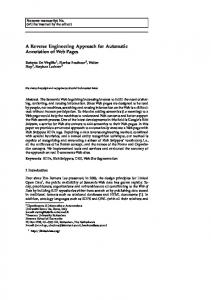
2. Statement of Two Illustrative Problems Our technique for automatically creating (reverse engineering) both the topology and sizing of a network of chemical reactions will be demonstrated herein by means of two illustrative problems. The first network (figure 1) consists of four reactions that are part of the phospholipid cycle, as presented in the E-CELL cell simulation model (Tomita, Hashimoto, Takahashi, Shimizu, Matsuzaki, Miyoshi, Saito, Tanida, Yugi, Venter, and Hutchison 1999). The first network’s external inputs (shown at the top of the figure) are glycerol (C00116) and fatty acid (C00162). The network also uses the cofactor ATP(C00002) (shown in the top right part of the figure). This network’s final product is diacyl-glycerol (C00165) (shown in the bottom left part of the figure). This network’s has four reactions (shown as rectangles in the figure). The four reactions are catalyzed by Glycerol kinase (EC2.7.1.30), Glycerol-1-phosphatase (EC3.1.3.21), Acylglycerol lipase (EC3.1.1.23), and Triacylglycerol lipase (EC3.1.1.3). The EC numbers are the codes assigned by the Enzyme Nomenclature Commission (Webb 1992). The reaction catalyzed by Acylglycerol lipase (EC3.1.1.23) and the reaction catalyzed by Triacylglycerol lipase (EC3.1.1.3) each have two substrates and one product. In figure 1, the reaction catalyzed by Glycerol kinase (EC2.7.1.30) has two substrates and two products. In figure 1, the reaction catalyzed by Glycerol-1-phosphatase (EC3.1.3.21) has one substrate and two products. This network (figure 1) has two intermediate substances, namely sn-Glycerol-3-Phosphate (C00093) and Monoacyl-glycerol (C01885), that are produced and consumed within the network. In this network (figure 1), the external supply of fatty acid (C00162) (shown at the top left in the figure) is distributed to two reactions (both on the left side of the figure), namely the reaction catalyzed by Acylglycerol lipase (EC3.1.1.23) and the reaction catalyzed by Triacylglycerol lipase (EC3.1.1.3). The external supply of glycerol (C00116) (shown at the top right in the figure) is distributed to two reactions, namely the reaction catalyzed by Glycerol kinase (EC2.7.1.30) and the reaction catalyzed by Glycerol-1-phosphatase (EC3.1.3.21). That is, both fatty acid (C00162) and glycerol (C00116) are each consumed by two reactions. This network of chemical reactions has two instances of a bifurcation point (where one substance is distributed to two different reactions). In addition, in this network (figure 1), the concentration of glycerol (C00116) is increased in two ways. First, as previously mentioned, it is externally supplied. Second, it is produced by the reaction catalyzed by Glycerol-1-phosphatase (EC3.1.3.21). That is, this network of chemical reactions has an instance of an accumulation point (where one substance is accumulated from two sources).

Also, this network (figure 1) of chemical reactions has an internal feedback loop in which a substance is both consumed and produced by the reactions in the loop. Specifically, glycerol (C00116) is consumed (in part) by the reaction catalyzed by Glycerol kinase (EC2.7.1.30). This reaction, in turn, produces an intermediate substance, snGlycerol-3-Phosphate (C00093). This intermediate substance is, in turn, consumed by the reaction catalyzed by Glycerol-1-phosphatase (EC3.1.3.21). That reaction, in turn, produces glycerol (C00116). An oval is used to indicate a point for measuring the concentration of each intermediate substance in this figure. In addition, an oval is also used for each bifurcation point and each accumulation point. When there is both a bifurcation point and an accumulation point for one particular substances (such as glycerol in this figure), one oval is used. The rate, K, of each of the four reactions in figure 1 is specified by a numerical constant contained in the rectangle representing the reaction. For example, the rate of reaction catalyzed by Acylglycerol lipase (EC3.1.1.23) is 1.95. The rate of reaction catalyzed by Triacylglycerol lipase (EC3.1.1.3) is 1.45. The rate of reaction catalyzed by Glycerol kinase (EC2.7.1.30) is 1.69. The rate of reaction catalyzed by Glycerol-1-phosphatase (EC3.1.3.21) is 1.19.

C00162 Fatty Acid

C00116

EC3.1.1.23 K = 1.95

C00162

Glycerol

Glycerol Acylglycerol lipase

C00116

EC3.1.3.21 K = 1.19

C01885

ATP

Glycerol-1phosphatase

C00002

EC2.7.1.30 K = 1.69

Glycerol kinase

Monoacylglycerol

Fatty Acid

EC3.1.1.3 K = 1.45

OUTPUT C00165 (MEASURED)

C00093 Triacylglycerol lipase

Diacyl-glycerol

sn-glycerol3phosphate

C00008 ADP

C00009 Orthophosphate

Cell Membrane

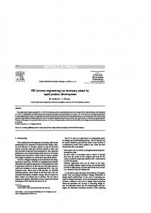
Figure 1 Four reactions from the phospholipid cycle. The second network (figure 2) consists of three reactions that are involved in the synthesis and degradation of ketone bodies. This network’s external inputs are Acetoacetyl-CoA and Acetyl-CoA. This network’s final product is Acetoacetate. The second network (figure 2) has three reactions. The three reactions are catalyzed by 3-oxoacid CoAtransferase (EC 2.8.3.5), Hydroxymethylglutaryl-CoA synthase (EC 4.1.3.5), and Hydroxymethylglutaryl-CoA lyase (EC 4.1.3.4). One of this network’s reactions (i.e., the reaction catalyzed by 3-oxoacid CoA-transferase (EC 2.8.3.5)) is a one-substrate, one-product reaction. The other two reactions are two-substrate, one product reactions. There is one intermediate substance, INT-1, in this network. Like the network for the first illustrative network of chemical reactions, this second illustrative network (figure 2) also incorporates three noteworthy topological features. First, this second network of chemical reactions has one instance of a bifurcation point (where one substance is distributed to two different reactions), namely for the externally supplied substance Acetoacetyl-CoA (in the upper left part of the figure).

Acetoacetyl -CoA

AcetylCoA

AcetoacetylCoA

AcetylCoA HydroxymethylglutarylCoA lyase EC4.1.3.5 EC4.1.3.4 K = 0.85 K = 0.70 HydroxymethylglutarylCoA synthase INT-1

EC2.8.3.5 K = 1.56 3-oxoacid CoAtransferase

Acetoacetate OUTPUT (MEASURED) Figure 2 Three reactions involved in the synthesis and degradation of ketone bodies. Second, this second network has two accumulation points. Acetyl-CoA (at the top of the figure) is an externally supplied substance and it is also produced by the reaction catalyzed by Hydroxymethylglutaryl-CoA lyase (EC 4.1.3.4). Also, the network’s final product, Acetoacetate (at the bottom of the figure) is produced by the reaction catalyzed by 3-oxoacid CoA-transferase (EC 2.8.3.5) and by the reaction catalyzed by Hydroxymethylglutaryl-CoA lyase (EC 4.1.3.4). Third, this second network has an internal feedback loop (in which a substance is both consumed and produced by the reactions in the loop). Specifically, Acetyl-CoA is consumed by the reaction catalyzed by Hydroxymethylglutaryl-CoA synthase (EC 4.1.3.5). This reaction, in turn, produces an intermediate substance (INT-1). This intermediate substance is, in turn, consumed by the reaction catalyzed by HydroxymethylglutarylCoA lyase (EC 4.1.3.4). That reaction, in turn, produces Acetyl-CoA.

3. Background on Genetic Programming Genetic programming is described in the book Genetic Programming: On the Programming of Computers by Means of Natural Selection (Koza 1992; Koza and Rice 1992), the book Genetic Programming II: Automatic Discovery of Reusable Programs (Koza 1994a, 1994b), and the book Genetic Programming III: Darwinian Invention and Problem Solving (Koza, Bennett, Andre, and Keane 1999; Koza, Bennett, Andre, Keane, and Brave 1999). Additional information on genetic programming can be found in books such as Banzhaf, Nordin, Keller, and Francone 1998; books in the series on genetic programming from Kluwer Academic Publishers such as Langdon 1998, Ryan 1999, and Wong and Leung 2000; in edited collections of papers such as the Advances in Genetic Programming series of books from the MIT Press (Kinnear 1994; Angeline and Kinnear 1996; Spector, Langdon, O’Reilly, and Angeline 1999); in the proceedings of the Genetic Programming Conference held between 1996 and 1998 (Koza, Goldberg, Fogel, and Riolo 1996; Koza, Deb, Dorigo, Fogel, Garzon, Iba, and Riolo 1997; Koza, Banzhaf, Chellapilla, Deb, Dorigo, Fogel, Garzon, Goldberg, Iba, and Riolo 1998); in the proceedings of the annual Genetic and Evolutionary Computation Conference (combining the annual Genetic Programming Conference and the International Conference on Genetic Algorithms) held starting in 1999 (Banzhaf, Daida, Eiben, Garzon, Honavar, Jakiela, and Smith, 1999; Whitley, Goldberg, Cantu-Paz, Spector, Parmee, and Beyer 2000); in the proceedings of the annual Euro-GP conferences held starting in 1998 (Banzhaf, Poli, Schoenauer, and Fogarty 1998; Poli, Nordin, Langdon, and Fogarty 1999; Poli, Banzhaf, Langdon, Miller, Nordin, and Fogarty 2000); at web sites such as www.genetic-programming.org; and in the Genetic Programming and Evolvable Machines journal (from Kluwer Academic Publishers).

Genetic programming is an extension of the genetic algorithm (Holland 1975) in which the population being bred consists of computer programs. Genetic programming breeds computer programs to solve problems by executing the following three steps: (1) Generate an initial population of compositions (typically random) of the functions and terminals of the problem. (2) Iteratively perform the following substeps (referred to herein as a generation) on the population of programs until the termination criterion has been satisfied: (A) Execute each program in the population and assign it a fitness value using the fitness measure. (B) Create a new population of programs by applying the following operations. The operations are applied to program(s) selected from the population with a probability based on fitness (with reselection allowed). (i) Reproduction: Copy the selected program to the new population. (ii) Crossover: Create a new offspring program for the new population by recombining randomly chosen parts of two selected programs. (iii) Mutation: Create one new offspring program for the new population by randomly mutating a randomly chosen part of the selected program. (iv) Architecture-altering operations: Select an architecture-altering operation from the available repertoire of such operations and create one new offspring program for the new population by applying the selected architecture-altering operation to the selected program. (3) Designate the individual program that is identified by result designation (e.g., the best-so-far individual) as the result of the run of genetic programming. This result may be a solution (or an approximate solution) to the problem. The individual programs that are evolved by genetic programming are typically multi-branch programs consisting of one or more result-producing branches and zero, one, or more automatically defined functions (subroutines). The architecture of such a multi-branch program involves (1) the total number of automatically defined functions, (2) the number of arguments (if any) possessed by each automatically defined function, and (3) if there is more than one automatically defined function in a program, the nature of the hierarchical references (including recursive references), if any, allowed among the automatically defined functions. Architecture-altering operations enable genetic programming to automatically determine the number of automatically defined functions, the number of arguments that each possesses, and the nature of the hierarchical references, if any, among such automatically defined functions.

4. Examples of Automatic Synthesis of Networks using Genetic Programming While it might seem difficult or impossible to automatically infer both the topology and numerical parameters for a complex network merely from observed data, recent work in several different fields has demonstrated that genetic programming can automatically create complex networks that exhibit prespecified behavior. The networks include those whose behavior is modeled by differential equations (both linear and non-linear) or by other equations (e.g., Maxwell’s equations for antennas). To make the above assertion concrete, the remainder of this section discusses three specific fields in which genetic programming has been shown to be capable of automatically inferring both the topology and numerical parameters for a complex network merely from observed data, namely • automatic synthesis of analog electrical circuits, • automatic synthesis of controllers, and • automatic synthesis of antennas.

4.1. Automatic Synthesis of Analog Electrical Circuits The design process entails creation of a complex structure to satisfy user-defined requirements. The design process for electrical circuits begins with a high-level description of the circuit’s desired behavior and entails creation of both the topology and the sizing of a satisfactory circuit. The topology of an electrical circuit comprises • the total number of electrical components, in the circuit, • the type of each component (e.g., resistor, capacitor, transistor) at each location in the circuit, and • a list of all the connections between the components. The sizing of a circuit consists of the component value(s) associated with each component. The sizing of a component is typically a numerical value (e.g., the capacitance of a capacitor). Considerable progress has been made in automating the design of certain categories of purely digital circuits; however, the design of analog circuits and mixed analog-digital circuits has not proved as amenable to automation. As Aaserud and Nielsen (1995) noted "[M]ost … analog circuits are still handcrafted by the experts or so-called 'zahs' of analog design. The design process is characterized by a combination of experience and intuition and requires a thorough knowledge of the process characteristics and the detailed specifications of the actual product. "Analog circuit design is known to be a knowledge-intensive, multiphase, iterative task, which usually stretches over a significant period of time and is performed by designers with a large portfolio of skills. It is therefore considered by many to be a form of art rather than a science." Genetic programming has, since 1995, been shown to be capable of automatically creating both the topology and sizing (component values) for analog electrical circuits composed of transistors, capacitors, resistors, and other components merely by specifying the circuit's output  that is, the output data values that would be observed if one already had the circuit. This automatic synthesis of circuits is performed by genetic programming even though there is no general mathematical method (prior to genetic programming) for creating (synthesizing) both the topology and sizing (component values) of analog electrical circuits from the circuit's desired (or observed) behavior (Aaserud and Nielsen 1995; Koza, Bennett, Andre, and Keane 1999). We discuss • a lowpass filter circuits using a fitness measure based on the frequency-domain behavior of circuits, and • a computational circuit employing transistors and using a fitness measure based on the time-domain behavior of circuits.

4.1.1. Lowpass Filter Circuit A simple filter is a one-input, one-output electronic circuit that receives a signal as its input and passes the frequency components of the incoming signal that lie in a specified range (called the passband) while suppressing the frequency components that lie in all other frequency ranges (the stopband). A lowpass filter passes all frequencies below a certain specified frequency, but stops all higher frequencies. A lowpass filter circuit is defined in terms of its behavior in response to input signals at various frequencies. Specifically, suppose 1,000 Hertz (Hz) is the boundary of the passband and 2,000 Hz is the boundary of the stopband of an illustrative lowpass filter. Figure 3 shows the output, in the time domain, of an illustrative lowpass filter that is receiving an input consisting of a 1,000-Hz 1-Volt sinusoidal signal (i.e., a signal right on the boundary of the passband). The horizontal axis represents time on a linear scale from 0 to 20 milliseconds. The vertical axis represents output voltage on a linear scale from –2.0 to +1.0 Volts.

Figure 3 Time domain behavior of a lowpass filter to a 1,000 Hz sinusoidal input signal. As can be seen, after a brief transient period of about five milliseconds (i.e., about five cycles of a 1,000 Hz signal), the circuit’s output (transient response) is an almost perfect 1,000 Hz sinusoidal signal with a full 1-Volt amplitude. That is, the lowpass filter passes the incoming 1,000-Hz signal at full power. Similarly, if we expose this lowpass filter circuit to a sinusoidal input signal at any frequency whatsoever below 1,000 Hz (say, 5 Hz, 50 Hz, or 500 Hz), we get (after a very brief transient period) a full-powered sinusoidal output signal at the same frequency as the incoming signal (i.e., 5 Hz, 50 Hz, or 500 Hz, respectively). Figure 4 shows the output of the illustrative lowpass filter in response to a 2,000 Hz 1-Volt sinusoidal input signal. Recall that 2,000 Hz is the boundary of the stopband of this lowpass filter. Notice that the vertical axis of this figure is in millivolts. As can be seen, after a brief transient period of about four milliseconds, the lowpass filter suppresses (attenuates) the incoming 1-Volt signal at 2,000 Hz to a tiny fraction of a Volt (i.e., almost zero).

Figure 4 Time domain behavior of a lowpass filter to a 2,000 Hz sinusoidal input signal.

Similarly, if we expose a lowpass filter circuit to any frequency whatsoever above 2,000 Hz (e.g., 5,000 Hz, 50,000 Hz), we get (after a very brief transient period) a similar nearly complete suppression of the incoming signal. That is, the lowpass filter suppresses all frequencies above the stopband’s boundary (at 2,000 Hz). In analyzing the behavior of filter, it is inconvenient to make multiple analyses of a circuit’s response in the time domain to a multiplicity of frequencies. Instead, given the intended frequency-sensitive function of a filer, it is far more convenient to view the behavior of a filter in the frequency domain. Figure 5 shows the frequency domain behavior of the same illustrative lowpass filter. The horizontal axis represents the frequency of the incoming signal and ranges over five decades of frequencies between 1 Hz and 100,000 Hz on a logarithmic scale. The vertical axis represents the peak voltage of the output and ranges between 0 to 1 Volts on a linear scale. This figure shows that when the input to the circuit consists of a sinusoidal signal with any frequency from 1 Hz to 1,000 Hz, the output is a sinusoidal signal with an amplitude of a full 1 Volt. This figure also shows that when the input to the circuit consists of a sinusoidal signal with any frequency from 2,000 Hz to 100,000 Hz, the amplitude of the output is essentially 0 Volts. The region between 1,000 Hz and 2,000 Hz is a transition region where the voltage varies between 1 Volts (at 1,000 Hz) and essentially 0 Volts (at 2,000 Hz).

Figure 5 Frequency domain behavior of a lowpass filter. Genetic programming is capable of automatically creating both the topology and sizing (component values) for lowpass filters (and other filter circuits, such as highpass filters, bandpass filters, bandstop filters, and filters with multiple passbands and stopbands). A filter circuit may be evolved using a fitness measure based on frequency domain behavior. In particular, the fitness of an individual circuit is the sum, over 101 values of frequency between 1 Hz and 100,000 Hz (equally space on a logarithmic scale), of the absolute value of the difference between the individual circuit’s output voltage and the ideal voltage for an ideal lowpass filter for that frequency (i.e., the voltages shown on figure 5). For example, one run of genetic programming synthesized the lowpass filter circuit of figure 6.

Figure 6 Lowpass filter created by genetic programming that infringes on Campbell’s patent.

The evolved circuit of figure 6 is what is now called a cascade (ladder) of identical π sections (Koza, Bennett, Andre, and Keane 1999, chapter 25). The evolved circuit has the recognizable topology of the circuit for which George Campbell of American Telephone and Telegraph received U. S. patent 1,227,113 in 1917. Claim 2 of Campbell’s patent covered, “An electric wave filter consisting of a connecting line of negligible attenuation composed of a plurality of sections, each section including a capacity element and an inductance element, one of said elements of each section being in series with the line and the other in shunt across the line, said capacity and inductance elements having precomputed values dependent upon the upper limiting frequency and the lower limiting frequency of a range of frequencies it is desired to transmit without attenuation, the values of said capacity and inductance elements being so proportioned that the structure transmits with practically negligible attenuation sinusoidal currents of all frequencies lying between said two limiting frequencies, while attenuating and approximately extinguishing currents of neighboring frequencies lying outside of said limiting frequencies.” In addition to possessing the topology of the Campbell filter, the numerical values of all the components in the evolved circuit closely approximate the numerical values taught in Campbell’s 1917 patent. Another run of genetic programming synthesized the lowpass filter circuit of figure 7. As before, this circuit was evolved using the previously described fitness measure based on frequency domain behavior.

Figure 7 Lowpass filter created by genetic programming that infringes on Zobel’s patent. This evolved circuit differs from the Campbell filter in that its final section consists of both a capacitor and inductor. This filter is an improvement over the Campbell filter because its final section confers certain performance advantages on the circuit. This circuit is equivalent to what is called a cascade of three symmetric T-sections and an M-derived half section (Koza, Bennett, Andre, and Keane 1999, chapter 25). Otto Zobel of American Telephone and Telegraph Company invented and received a patent for an “M-derived half section” used in conjunction with one or more “constant K” sections. Again, the numerical values of all the components in this evolved circuit closely approximate the numerical values taught in Zobel's 1925 patent. Seven circuits created using genetic programming infringe on previously issued patents ((Koza, Bennett, Andre, and Keane 1999). Others duplicate the functionality of previously patented inventions in novel ways. In both of the foregoing examples, genetic programming automatically created both the topology and sizing (component values) of the entire filter circuit by using a fitness measure expressed in terms of the signal observed at the single output point (the probe point labeled VOUT in the figures).

4.1.2. Squaring Computational Circuit Because filters discriminate on incoming signals based on frequency, the lowpass filter circuit was automatically synthesized using a fitness measure based on the behavior of the circuit in the frequency domain. However, for many circuits, it is appropriate to synthesize the circuit using a fitness measure based on the behavior of the circuit in the time domain. An analog electrical circuit whose output is a well-known mathematical function (e.g., square, square root) is called a computational circuit. Figure 8 shows a squaring circuit composed of transistors, capacitors, and resistors that was automatically synthesized using a fitness measure based on the behavior of the circuit in the time domain (Mydlowec and Koza 2000).

Figure 8 Squaring circuit created by genetic programming. This circuit was evolved using a fitness measure based on time-varying input signals. In particular, fitness was the sum, taken at certain sampled times for four different time-varying input signals, of the absolute value of the difference between the individual circuit’s output voltage and the desired output voltage (i.e., the square of the voltage of the input signal at the particular sampled time). The four input signals were structured to provide a representative mixture of input values. All of the input signals produce outputs that are well within the range of voltages that can be handled by transistors (i.e., below 4 volts). Figure 9 shows one of the input signals, namely a rising ramp.

4.0

3.0

Voltage

2.0

1.0

0.0

-1.0

-2.0 0.0

0.2

0.4

0.6

0.8

1.0

Time

Figure 9 Rising ramp. Figure 10 shows the output voltage produced by the evolved circuit for the rising ramp input superimposed on the (virtually indistinguishable) correct output voltage for the squaring function. As can be seen, as soon as the input signal becomes non-zero, the output is a parabolic-shaped curve representing the square of the incoming voltage.

4.0

3.0

Voltage

2.0

1.0

0.0

-1.0

-2.0 0.0

0.2

0.4

0.6

0.8

1.0

Time

Figure 10 Output for rising ramp input for squaring circuit.

4.2. Automatic Synthesis of Controllers The purpose of a controller is to force, in a meritorious way, the actual response of a system (conventionally called the plant) to match a desired response (called the reference signal) (Dorf and Bishop 1998). Controllers are typically composed of signal processing blocks, such as integrators, differentiators, leads, lags, delays, gains, adders, inverters, subtractors, and multipliers. The topology of a controller comprises • the total number of signal processing blocks in the controller, • the type of each block (e.g., integrator, differentiator, lead, lag, delay, gain, adder, inverter, subtractor, and multiplier), • the connections between the inputs and output of each block in the controller and the external input and external output points of the controller. The tuning (sizing) of a controller consists of the parameter values associated with each signal processing block. Genetic programming is capable of automatically creating both the topology and sizing (tuning) for controllers composed of time-domain blocks merely by specifying the controller’s effect on the to-be-controlled plant (Keane, Yu, and Koza 2000; Koza, Keane, Yu, Bennett, Mydlowec, and Stiffelman 1999; Koza, Keane, Bennett, Yu, Mydlowec, and Stiffelman, Oscar 1999; Koza, Keane, Yu, Bennett, and Mydlowec 2000; Koza, Keane, Yu, Mydlowec, and Bennett 2000a, 2000b; Koza, Yu, Keane, and Mydlowec 2000; Yu, Keane, and Koza. 2000). This automatic synthesis of controllers from data is performed by genetic programming even though there is no general mathematical method for creating both the topology and sizing for controllers from a high-level statement of the design goals for the controller. In the PID type of controller, the controller’s output is the sum of the output of three terms  a proportional (P) term, an integrative (I) term, and a derivative (D) term. The difference between the plant’s output and the reference signal is the input to the proportional, integrative, and derivative blocks. Albert Callender and Allan Stevenson of Imperial Chemical Limited of Northwich, England received U.S. Patent 2,175,985 in 1939 for the PI and PID controller. Claim 1 of the patent issued to Callender and Stevenson (1939) covers what is now called the PI controller and states, "A system for the automatic control of a variable characteristic comprising means proportionally responsive to deviations of the characteristic from a desired value, compensating means for adjusting the value of the characteristic, and electrical means associated with and actuated by responsive variations in said responsive means, for operating the compensating means to correct such deviations in conformity with the sum of the extent of the deviation and the summation of the deviation."

Claim 3 of Callender and Stevenson (1939) covers what is now called the PID controller, "A system as set forth in claim 1 in which said operation is additionally controlled in conformity with the rate of such deviation." The vast majority of automatic controllers used by industry are of the PI or PID type. However, it is generally recognized by leading practitioners in the field of control that PI and PID controllers are not ideal (Astrom and Hagglund 1995; Boyd and Barratt 1991). There is no preexisting general-purpose analytic method (prior to genetic programming) for automatically creating both the topology and tuning of a controller for arbitrary linear and non-linear plants that can simultaneously optimize prespecified performance metrics. The performance metrics used in the field of control include, among others, • minimizing the time required to bring the plant output to the desired value (as measured by, say, the integral of the time-weighted absolute error), • satisfying time-domain constraints (involving, say, overshoot and disturbance rejection), • satisfying frequency domain constraints (e.g., bandwidth), and • satisfying additional constraints, such as limiting the magnitude of the control variable or the plant’s internal state variables. We employ a problem involving control of a two-lag plant (described by Dorf and Bishop 1998, page 707) to illustrate the automatic synthesis of controllers by means of genetic programming. The problem entails synthesizing the design of both the topology and parameter values for a controller for a two-lag plant such that plant output reaches the level of the reference signal so as to minimize the integral of the time-weighted absolute error, such that the overshoot in response to a step input is less than 2%, and such that the controller is robust in the face of significant variation in the plant’s internal gain, K, and the plant’s time constant, τ. Genetic programming routinely creates PI and PID controllers infringing on the 1942 of Callender and Stevenson patent during intermediate generations of runs of genetic programming on controller problems. However, the PID controller is not the best possible controller for this (and many) problems. Figure 11 shows the block diagram for the best-of-run controller evolved during one run of this problem. In this figure, R(s) is the reference signal; Y(s) is the plant output; and U(s) is the controller’s output (control variable). This evolved controller is 2.42 times better than the Dorf and Bishop (1998) controller as measured by the criterion used by Dorf and Bishop. In addition, this evolved controller has only 56% of the rise time in response to the reference input, has only 32% of the settling time, and is 8.97 times better in terms of suppressing the effects of disturbance at the plant input. R(s)

1 1 + 0.168s

1 1 + 0.156 s

Y(s)

1 + 0.515s

−1

1 s

−1

−1

8.15

U(s)

918.8

1 + 0.0385 s

1 + 0.0837 s

Figure 11 Evolved controller that infringes on Jones’ patent. This genetically evolved controller differs from a conventional PID controller in that it employs a second derivative processing block. Specifically, after applying standard manipulations to the block diagram of this evolved controller, the transfer function for the best-of-run controller can be expressed as a transfer function for a pre-filter and a transfer function for a compensator. The transfer function for the pre-filter, Gp32(s), for the best-of-run individual from generation 32 is

G p32 ( s) =

1(1 + .1262s)(1 + .2029s) (1 + .03851s)(1 + .05146)(1 + .08375)(1 + .1561s)(1 + .1680s)

The transfer function for the compensator, Gc32(s), is 7487(1 + .03851s )(1 + .05146s )(1 + .08375s ) 7487.05 + 1300.63s + 71.2511s 2 + 1.2426s 3 = s s 3 The s term (in conjunction with the s in the denominator) indicates a second derivative. Thus, the compensator consists of a second derivative in addition to proportional, integrative, and derivative functions. As it happens, Harry Jones of The Brown Instrument Company of Philadelphia received U. S. Patent 2,282,726 for this kind of controller topology in 1942. Claim 38 of the Jones patent (Jones 1942) states, Gc32 ( s) =

"In a control system, an electrical network, means to adjust said network in response to changes in a variable condition to be controlled, control means responsive to network adjustments to control said condition, reset means including a reactance in said network adapted following an adjustment of said network by said first means to initiate an additional network adjustment in the same sense, and rate control means included in said network adapted to control the effect of the first mentioned adjustment in accordance with the second or higher derivative of the magnitude of the condition with respect to time." Note that the human user of genetic programming did not preordain, prior to the run (i.e., as part of the preparatory steps for genetic programming), that a second derivative should be used in the controller (or, from that matter, even that a P, I, or D block should be used). Genetic programming automatically discovered that the second derivative element (along with the P, I, and D elements) were useful in producing a good controller for this particular problem. That is, necessity was the mother of invention. Similarly, the human who initiated this run of genetic programming did not preordain any particular topological arrangement of proportional, integrative, derivative, second derivative, or other functions within the automatically created controller. Instead, genetic programming automatically created a controller for the given plant without the benefit of user-supplied information concerning the total number of processing blocks to be employed in the controller, the type of each processing block, the topological interconnections between the blocks, the values of parameters for the blocks, or the existence of internal feedback (none in this instance) within the controller.

4.3. Automatic Synthesis of Antennas An antenna is a device for receiving or transmitting electromagnetic waves. An antenna may receive an electromagnetic wave and transform it into a signal on a transmission line. Alternately, an antenna may transform a signal from a transmission line into an electromagnetic wave that is then propagated in free space. Maxwell’s equations govern the electromagnetic waves generated and received by antennas. The behavior and characteristics of many antennas can be determined by simulation. For example, the Numerical Electromagnetics Code (NEC) is a method-of-moments (MoM) simulator for wire antennas that was developed at the Lawrence Livermore National Laboratory (Burke 1992). The task of analyzing the characteristics of a given antenna is difficult. The task of synthesizing the design of an antenna with specified characteristics typically calls for considerable creativity on the part of the antenna engineer (Balanis 1982; Stutzman and Thiele 1998; Linden 1997). Genetic programming is capable of discovering both the topological and numerical aspects of a satisfactory antenna design from a high-level specification of the antenna’s behavior. In one particular problem (Comisky, Yu, and Koza 2000), genetic programming automatically discovered the design for a satisfactory antenna composed of wires for maximizing gain in a preferred direction over a specified range of frequencies, having a reasonable value of voltage standing wave ratio when the antenna is fed by a transmission line with a specified characteristic impedance, and fitting into a specified bounding rectangle. The design discovered by genetic programming included (1) the number of directors in the antenna, (2) the number of reflectors, (3) the fact that the driven element, the directors, and the reflector are all single straight wires, (4) the fact that the driven element, the directors, and the reflector are all arranged in parallel, (5) the fact that the energy source (via the transmission line) is connected only to the driven element  that is, the directors and reflectors are parasitically coupled.

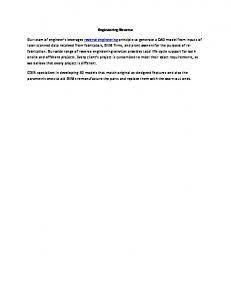
The last three of the above characteristics discovered by genetic programming are the defining characteristics of an inventive design conceived in the early years of the field of antenna design (Uda 1926, 1927; Yagi 1928). Figure 12 shows the antenna created by genetic programming. It is an example of what is now called a Yagi-Uda antenna. It is approximately the same length as the conventional Yagi-Uda antenna that a human designer might develop in order to satisfy this problem’s requirements (concerning gain).

y(m)

0.2 0 0.2 0

0.5

1 x(m)

1.5

2

Figure 12 Antenna design created by genetic programming.

5. Types of Chemical Reactions A chemical reaction typically causes a change, over time, in the concentration of the various substances participating in the reaction. Chemical reactions involve substances and reactions. Substances include reactants (input substances), intermediate products, and products (output substances). A substance often appears as both a reactant and product in a network or reactions. The rate of many chemical reactions is affected by a catalyst (a substance that accelerates or decelerates the rate of a reaction, but remains unchanged by the reaction). In a living cell, the catalysts are often enzymes. The reactant(s) of a catalyzed reaction are usually called substrate(s).

5.1. One-Substrate, One-Product Reaction First consider an illustrative chemical reaction in which one chemical (the substrate) is transformed into another chemical (the product) under control of a catalyst. Figure 13 shows an illustrative one-substrate, one-product chemical reaction in which pyrophosphate (the substrate) is transformed into orthophosphate (the product) under control of the catalyst pyrophosphatase (EC3.6.1.1). In this paper, C00013 is an alternative designation for pyrophosphate and that C00009 is an alternative designation for orthophosphate. This reaction (and the other illustrative reactions in this section) are all part of the nine reactions of the phospholipid cycle that is presented in the E-CELL cell simulation model (Tomita, Hashimoto, Takahashi, Shimizu, Matsuzaki, Miyoshi, Saito, Tanida, Yugi, Venter, and Hutchison 1999).

Pyrophosphate

C00013

Pyrophosphatase EC3.6.1.1-0

C00009

Orthophosphate Figure 13 An illustrative one-substrate, one-product chemical reaction.

Figure 14 shows a plot, over 60 seconds of time, of the concentrations of the three substances involved in the illustrative one-substrate, one-product enzymatic reaction for producing orthophosphate. The concentration of pyrophosphatase (the catalyst) is constant at 1.2 over the entire time period involved. The concentration of pyrophosphate (the substrate) starts at 1.0 (its concentration at time t = 0). As the substrate (pyrophosphate) is consumed by the reaction, its concentration decreases until it reaches a level of 0.0 at about t = 10 (and remains at this level thereafter). The concentration of the product (orthophosphate) starts at 0.0 (its concentration at time t = 0). As the product (orthophosphate) is produced by the reaction, its concentration increases to a level of 1.0 at about t = 10 (and remains at this level thereafter). Xa: 60.00 Yc: 1.200

V(5) V(12) V(9)

Xb: 0.000 Yd: 0.000

a-b: 60.00 c-d: 1.200

freq: 16.67m

b 1.2

a c

1 800m 600m 400m 200m 0 0

d 10

20

30 Ref=Ground X=10/Div Y=voltage

40

50

60

Figure 14 Changing concentrations of substances in an illustrative one-substrate, one-product reaction. The action of an enzyme (catalyst) in a one-substrate chemical reaction can be viewed as two-step process in which the enzyme E first binds with the substrate S at a rate k1 to form ES. The formation of the product P from ES then occurs at a rate k2. The reverse reaction (for the binding of E with S) in which ES dissociates into E and S, occurs at a rate of k-1. 1 → k2 ES → P+E ← k

k

E+S

−1

The rates of chemical reactions are modeled by rate laws. The concentrations of substrates, products, intermediate substances, and catalysts participating in reactions are modeled by various rate laws, including firstorder rate laws, second-order rate laws, power laws, and the Michaelis-Menten equations (Voit 2000). For example, the Michaelis-Menten rate law for a one-substrate chemical reaction is

d [ P] k 2 [ E ]0 [ S ]t = . dt [ S ]t + K m In this rate law, [P] is the concentration of the reaction’s product P; [S]t is the concentration of substrate S at time t; [E]0 is the concentration of enzyme E at time 0 (and at all other times); and Km is the Michaelis constant defined as

Km =

k −1 + k 2 . k1

However, when the constants Km and k2 are considerably greater than the concentrations of substances, it is often satisfactory to use a psuedo-first-order rate law such as

d [ P] k 2 [ E ]0 [ S ]t = = k new [ E ]0 [ S ]t , dt Km where Knew is a constant defined as

k new =

k2 . Km

The above psuedo-first-order rate law involves only multiplication. It is both convenient and useful to represent the behavior, over time, of a chemical reaction as an analog electrical circuit. In this representation, the concentration of a substance is represented as a voltage in the time domain. Figure 15 shows an electrical circuit representing the illustrative one-substrate-one-product enzymatic reaction.

EC3.6.1.1

Figure 15 Circuit for one-substrate, one-product chemical reaction. This circuit is composed of elements such as • voltage sources (represented by small circles such as V18 at the top left of the figure as well as voltage sources V20, V8, V1, and V2 elsewhere in the figure), • voltage adders with three ports (represented by rectangles and labeled ADDV, such as M21 at the top left of the figure as well as voltage adders M23 and M8 elsewhere in the figure), • sum-integrators (represented by a triangle-rectangle combination with three ports, such as U23 at the top left of the figure as well as sum-integrators U26 and U7 elsewhere in the figure), • a one-substrate chemical reaction element MICH_1 (represented by the rectangle U25 with five ports at the top right of the figure), • a ground point (at the bottom of the figure), and • an output point (represented by the dangling wire emanating from voltage adder M8 at the bottom middle of the figure and labeled as probe point 5). The initial concentration of pyrophosphate (the substrate) is 1.0, as established by the 1-volt voltage source V18 (in the top left part of figure 15). Voltage adder M21 (in the top left part of the figure) is an electrical component for adding two voltages. V18 is one of its two inputs. The output of voltage adder M21 represents the concentration of pyrophosphate (the substrate in this illustrative one-substrate-one-product reaction). Ignoring, for the moment, the second input port to voltage adder M21, the output of M21 goes into the port labeled "substrate" of the one-substrate reaction element MICH_1 labeled U25 (at the top right of the figure). If desired, this voltage representing the concentration of the substrate can be measured at probe point 9 of the circuit (along the line at the top of the figure). In figure 15, the element MICH_1 is an analog computational subcircuit that models the rate law being used. For example, the rate law may be the Michaelis-Menten law. Alternatively, the rate law may be a first-order rate law described above. Then again, the rate law may be some other rate law (Voit 2000). The constant, Km, goes into the port labeled Km of the reaction element MICH_1 of figure 15. Similarly, the constant k2 goes into the port labeled k2 of the reaction element MICH_1. The initial concentration of catalyst (pyrophosphatase) is 1.0 (established by the 1-volt voltage source V20 of voltage adder M23). The output of voltage adder M23 goes into the port labeled "enzyme" of the one-substrate, oneproduct reaction element MICH_1 labeled U25. If desired, this voltage can be measured at probe point 12.

The initial concentration of product (orthophosphate) is 0.0, as established by the 0-volt voltage source V8 of voltage adder M8. If desired, this voltage can be measured at probe point 5 (the dangling wire in the figure). U23, U26, and U7 are sum-integrators that integrate, over time, the sum of their respective two inputs. In each case in figure 15, one of the two incoming ports of each sum-integrator in the figure is negated, so that U23, U26, and U7 serve as differential-integrators. That is, they sum, over time, the difference of their two inputs. The output of the reaction element MICH_1 labeled U25 is the reaction’s rate. If desired, this reaction rate can be measured at probe point 4 (along the bottom of the figure). This reaction rate fed to • a subtractive input to sum-integrator U23, and • an additive input to sum-integrator U7. These two connections are of central importance in the figure. They reflect the conservation principle inherent in a chemical reaction. Specifically, the subtractive input to sum-integrator U23 reflects the fact that the substrate substance is consumed by the reaction at the specified rate, while the additive input to sum-integrator U7 reflects the fact that the product substance is produced by the reaction at the same specified rate. Since there is nothing in the figure that consumes any of the reaction’s product, the subtractive input to sumintegrator U7 is zero (i.e., grounded). Two-input voltage adder M8 adds the product’s initial concentration (0.0) (at probe 3) to the concentration (at probe 6) of the product that is being produced by the reaction. Since there is nothing in the figure that creates additional substrate, the additive input to sum-integrator U23 is zero (i.e., grounded). Thus, two-input voltage adder M21 adds the substrate’s initial concentration (1.0) (at probe 10) to the (negative) concentration (at probe 11) of the substrate that is being consumed by the reaction. There is one voltage source, one sum-integrator, and one voltage adder associated with the enzyme that catalyzes this reaction. Since the concentration of a catalyst is unchanged by a reaction, the additive and subtractive inputs to sum-integrator U26 are both zero (i.e., grounded). This sum-integrator could, of course, simply be deleted. However, we employ this consistent arrangement of three components (i.e., voltage source, sum-integrator, and voltage adder) in all the figures herein to emphasize the consistent formal procedure that we are using to translate a chemical reaction diagram into the electrical circuit. In practice, when both inputs of a sum-integrator are connected to ground, the sum-integrator is simply deleted from the circuit that is eventually simulated. SPICE is a large family of programs written over several decades at the University of California at Berkeley that was written for the purpose of simulating the behavior of analog, digital, and mixed analog/digital electrical circuits. SPICE3 (Quarles, Newton, Pederson, and Sangiovanni-Vincentelli 1994) is the most recent version of Berkeley SPICE. SPICE3 consists of about 217,000 lines of C source code residing in 878 separate files. The required input to the SPICE simulator consists of a netlist along with certain commands required by the SPICE simulator. The netlist describes the topology and parameter values of the electrical circuit that is to be simulated. SPICE is capable of simulating behavior in the time domain and the frequency domain (and in many other ways). We have embedded our modified version of SPICE as a submodule within our genetic programming system. Thus, we can readily invoke SPICE in order to ascertain the behavior of an electrical circuit. A diagram representing an electrical circuit differs from a diagram representing a network of chemical reactions in several important ways. In particular, there is no directionality of wires in circuits (as there is in the block diagram representing a network of chemical reactions). In addition, since SPICE was written for the purpose of simulating the behavior of electrical circuits, it does not have built-in components that correspond to chemical rate laws, such as a first-order rate law, a second-order rate law, a power law, or the Michaelis-Menten equations. However, these rate laws can be realized by using the facility of SPICE to create subcircuit definitions (macros). A subcircuit in SPICE may (or may not) contain real-world electrical components. Mathematical functions such as integration and differentiation can be realized by using electrical components such as capacitors and inductors. More importantly, SPICE has a facility for representing arbitrary continuous-time mathematical functions (regardless of whether there is any real-world electrical component, or any obvious combination of real-world components, to realize the function). Once a subcircuit is defined in SPICE, it operates as if it were an electrical component. Thus, it may be inserted into an electrical circuit along with other electrical components or other subcircuits. For example, voltage multiplication (XMULTV) can be realized by a subcircuit definition (macro). The subcircuit definition entails multiplying two voltages, V(1) and V(2) to produce an output voltage at node V(3). *NETLIST FOR SUBCIRCUIT DEFINITION OF VOLTAGE MULTIPLICATION (XMULTV) .SUBCKT XMULTV 1 2 3 BX 3 0 V=V(1)*V(2) .ENDS XMULTV Voltage multiplication can also be accomplished by means of a computational circuit for multiplication. However, the computational circuit necessary to realize a mundane mathematical function, such as multiplication, can be complicated and difficult to design (Gilbert 1968; Sheingold 1976; Babanezhad and Temes 1986).

Voltage addition (XADDV) can be realized in a similar manner by means of the following subcircuit definition: *NETLIST FOR SUBCIRCUIT DEFINITION OF VOLTAGE ADDITION (ADDV) .SUBCKT XADDV 1 2 3 BX 3 0 V=V(1)+V(2) .ENDS XADDV Similarly, voltage division (XDIVV) can be realized by the following subcircuit definition: *NETLIST FOR SUBCIRCUIT DEFINITION OF VOLTAGE DIVISION (DIVV) .SUBCKT XDIVV 1 2 3 BX 3 0 V=V(1)/V(2) .ENDS XDIVV Similarly, the pseudo-first-order rate law rate law can be realized in SPICE by a subcircuit definition (macro). The pseudo-first-order rate law XFORL ("First Order Rate Law") entails multiplying three voltages, V(1), V(2), and V(4) to produce an output voltage a node V(3). *NETLIST FOR SUBCIRCUIT DEFINITION OF PSEUDO-FIRST-ORDER RATE LAW (XFORL) .SUBCKT XFORL 1 2 3 4 BX 3 0 V=V(1)*V(2)*V(4) .ENDS The pseudo-second-order rate law rate law can be realized in SPICE by a subcircuit definition. The pseudosecond-order rate law XSORL ("Second Order Rate Law") entails multiplying four voltages, V(1), V(2), V(3), and V(5) to produce an output voltage a node V(4). *NETLIST FOR SUBCIRCUIT DEFINITION OF PSEUDO-SECOND-ORDER RATE LAW (XSORL) .SUBCKT XSORL 1 2 3 4 5 BX 4 0 V=V(1)*V(2)*V(3)*V(5) .ENDS As another example, a sum-integrator (SUMINT) can be realized in SPICE by the following subcircuit definition (employing a one giga-Ohm resistor R2 and a capacitor C1 with an initial condition, IC, of 0 volts): *NETLIST FOR SUMINTEGRATOR (SUMINT) .SUBCKT SUMINT 1 2 3 4 G1 4 0 1 2 1.0 C1 4 0 1.0 IC=0.0 R2 4 0 1000.0MEG UNARYV 3 0 V=-V(4) .ENDS Figure 16 shows a subcircuit for a sum-integrator SUMINT. The symbol for the sum-integrator is shown at the top of the figure in the form of a triangle-rectangle combination. The sum-integrator has two input ports (one with a positive sign and one with a negative sign). Its one output (node 3) is the integral of the difference of its two inputs. The circuit required to implement a sum-integrator consists of a voltage-controlled current source (in the lower left corner of the figure), a capacitor C1, a resistor R2, and an inverter UNARYV (the rectangle in the middle of the right side of the figure). The rounded box on the right side of the figure represents the initial condition (i.e., initial charge) on the capacitor C1. The voltage-controlled current source converts the difference in the two voltages to a current. The capacitor C1 (starting with its initial charge) integrates the current. The capacitor voltage (node 4) is equal to the total charge (i.e., the integral of the current) divided by its capacitance. The Michaelis-Menten equations can also be realized by an electrical circuit. Figure 17 shows a circuit for the one-substrate Michaelis-Menten equation MICH_1

d [ P] k 2 [ E ]0 [ S ]t = . dt [ S ]t + K m using two voltage multiplications XMULTV, a voltage addition ADDV, and a voltage division XDIVV.

Figure 16 Sum-integrator.

Figure 17 Subcircuit for one-substrate Michaelis-Menten equation MICH_1. The subcircuit definition in SPICE for the one-substrate Michaelis-Menten equation MICH_1 is as follows: *NETLIST FOR MICHAELIS-MENTEN MICH_1 XXM4 4 3 2 XDIVV XXM3 6 5 3 XADDV XXM2 7 8 4 XMULTV XXM1 9 5 8 XMULTV .SAVE V(2) V(3) V(4) V(5) V(6) V(7) V(8) V(9) .END When the user-defined macro for the differential-integrator and the user-defined macro for the one-input reaction element are combined, the resulting netlist is as follows: *NETLIST FOR 1-1-REACTION IN PHOSPHOLIPID-CIRCUIT XXM1#1 15 6 XUNARYV

GVCIS1#2 15 0 4 0 1 C1#3 0 15 1 XXM8 3 6 5 XADDV V8 3 0 DC 0 V2 7 0 DC 0.2V V1 8 0 DC 0.2V XXM1#4 16 11 XUNARYV GVCIS1#5 16 0 0 4 1 C1#6 0 16 1 XXM21 10 11 9 XADDV V18 10 0 DC 1V XXM1#7 17 13 XUNARYV GVCIS1#8 17 0 0 0 1 C1#9 0 17 1 XXM4#10 19 18 4 XDIVV XXM3#11 7 9 18 XADDV XXM2#12 8 20 19 XMULTV XXM1#13 12 9 20 XMULTV XXM23 14 13 12 XADDV V20 14 0 DC 1V R2#14 0 15 1000MEG R2#15 0 16 1000MEG R2#16 0 17 1000MEG .IC V(15)=0V V(16)=0V V(17)=0V .SAVE V(3) V(4) V(5) V(6) V(7) V(8) V(9) V(10) V(11) V(12) V(13) V(14) @V8[P] .SAVE V8#BRANCH @V2[P] V2#BRANCH @V1[P] V1#BRANCH @V18[P] V18#BRANCH @V20[P] .SAVE V20#BRANCH *BKGND=RGB 0 0 0 *BINARY RAW FILE * * SELECTED CIRCUIT ANALYSES : .TRAN 10M 60 0 10M * * MODELS/SUBCIRCUITS USED: * *UNARYV UNARY MINUS OF VOLTAGE -- PKG:-(V) .SUBCKT XUNARYV 1 2 BX 2 0 V=-(V(1)) .ENDS XUNARYV * *ADDV ADD VOLTAGES -- PKG:V(A+B) .SUBCKT XADDV 1 2 3 BX 3 0 V=V(1)+V(2) .ENDS XADDV * *DIVV DIVIDE VOLTAGES -- PKG:V(A/B) .SUBCKT XDIVV 1 2 3 BX 3 0 V=V(1)/V(2) .ENDS XDIVV * *MULTV MULTIPLY VOLTAGES -- PKG:V(A*B) .SUBCKT XMULTV 1 2 3 BX 3 0 V=V(1)*V(2) .ENDS XMULTV * .END

5.2. One-Substrate, Two-Product Reaction Figure 18 shows an illustrative one-substrate, two-product chemical reaction in which Phosphatidylglycerophosphate (the substrate) is transformed into orthophosphate and Phosphotidylglycerol (the two products) under control of phosphatidylglycerophosphatase (the catalyst). The catalyst in this reaction is the enzyme

pyrophosphatase (EC3.1.3.27). Note that C03892 is an alternative designation herein for Phosphatidylglycerophosphate; that C00009 is an alternative designation for orthophosphate; and that C00344 is an alternative designation for Phosphotidylglycerol. Orthophosphate C00009

C03892

Phosphatidylglycerophosphate

EC3.1.3.27-0

Phosphatidylglycerophosphatase

C00344

Phosphotidylglycerol

Figure 18 Illustrative one-substrate, two-product reaction. This illustrative one-substrate, two-product chemical reaction can be represented as a circuit in a manner similar to that just described in the previous section for a one-substrate, one-product reaction. Figure 19 shows an electrical circuit representing a one-substrate-two-product enzymatic reaction. This circuit is composed of • voltage sources V23, V24, V25, V8, V2, and V1, • voltage adders with three ports M27, M29, M30, and M8, • sum-integrators U27, U32, U33, and U7, • a one-substrate chemical reaction element MICH_1, • a ground point (at the bottom of the figure), and • two output points (represented by the dangling wires emanating from voltage adders M30 and M8 at the bottom middle of the figure). • has one voltage adder M27 (representing the one substrate of this reaction), • has two voltage adders M30 and M8 (representing the two products of this reaction) and a dangling wire for each of the two products of the reaction, and • the "rate" output of the reaction element MICH_1 is connected to the negative lead to sum-integrator U27 (representing the one substrate) to establish that one substrate is consumed by the reaction. • the "rate" output of the reaction element MICH_1 is connected to the positive lead to sum-integrators U33 and U7 (representing the two products) to establish that two products are produced by the reaction.

EC3.1.3.27

Figure 19 Circuit for illustrative one-substrate, two-product chemical reaction. As before, there is one voltage source, sum-integrator, and voltage adder associated with the enzyme that catalyzes this reaction. Both the positive and negative leads of this sum-integrator are grounded to reflect the fact that the concentration of the enzyme remains unchanged during the reaction.

5.3. Two-Substrate, One-Product Reaction Figure 20 shows an illustrative two-substrate, one-product chemical reaction in which fatty acid (C00162) and Glycerol (C00116) (the two substrates) are transformed into Monoacyl-glycerol (C01885) (the product) under control of Acylglycerol_lipase (EC3.1.1.23) (the catalyst).

Fatty Acid C00162

Acylglycerol Lipase

Glycerol

EC3.1.1.23-0 C00116

C01885

Monoacyl-glycerol

Figure 20 Illustrative two-substrate, one-product reaction. The action of an enzyme (catalyst) in a two-substrate chemical reaction can be viewed as two-step process in which the enzyme E first binds with the substrates A and B at a rate k1 to form ABE. The reverse reaction, in which ABE dissociates into E, A, and B occurs at a rate of k-1. The formation of the product P from EAB then occurs at a rate k2.

1 → k2 ABE → P+E ← k

k

E + A+ B=

−1

The Michaelis-Menten rate law for a two-substrate chemical reaction is

Ratet =

[ E ]0 . 1 1 1 1 + + + K 0 K A [ A]t K B [ B]t K AB [ A]t [ B]t

However, when k-1 ~ 0 and k-1