be used in conjunction with hybrid Monte Carlo methods because these require strictly reversible molecular dynamics in order to satisfy detailed balance.4.
Reversible
multiple
M. Tuckermar?)
time scale molecular
dynamics
and B. J. Berne
Department of Chemistry, Columbia University, New York, New York 10027
G. J. Martyna Department of Chemistry, University of Pennsylvania, Philadelphia, Pennsylvania 19104-6323
(Received 13 January 1992; accepted 17 March 1992) The Trotter factorization of the Liouville propagator is used to generate new reversible molecular dynamics integrators. This strategy is applied to derive reversible reference system propagator algorithms (RESPA) that greatly accelerate simulations of systems with a separation of time scales or with long range forces. The new algorithms have all of the advantages of previous RESPA integrators but are reversible, and more stable than those methods. These methods are applied to a set of paradigmatic systems and are shown to be superior to earlier methods. It is shown how the new RESPA methods are related to predictorcorrector integrators. Finally, we show how these methods can be used to accelerate the integration of the equations of motion of systems with Nose thermostats.
1. INTRODUCTION Recently we have devised reference system algorithms for treating problems with separation in time scales (stiff oscillators in soft fluids,’ disparate masses’) and/or forces that can be separated into short and long range components3 ). These algorithms run at much faster speeds than do the standard algorithms; sometimes with speedup factors on the order of 20 to 30. Some of these reference system methods are not reversible in time, and thus may exhibit numerical instabilities after very long times. Moreover, they can not be used in conjunction with hybrid Monte Carlo methods because these require strictly reversible molecular dynamics in order to satisfy detailed balance.4 In this paper we show how to make these reference system algorithms reversible in time. The starting point is the Trotter expansion of the classical Liouville propagate?’ and the reversable Trotter expansion.” From this we derive several new integrators for solving Newton’s equations of motion. These new integration schemes involve the same number of force evaluations as the methods previously introduced, and therefore require no more CPU time in their execution. Furthermore, we find that making these methods reversible in time increases their stability over the RESPA and NAPA methods previously introduced. In Sec. II we present a necessary review of the Liouville operator formalism. Trotter factorizations of the classical propagator can be used to derive simple integrators. In Sec. II A the velocity Verlet integrator as well as a new integrator, the position Verlet integrator is derived. In Sec. II C generalized Trotter factorizations are introduced. In Sec. III we treat the long range force problem and apply it to a particular example. In Sec. IV we treat the multiple time scale problem and apply it to the disparate mass mixtures in Sec. IV A and to systems with stiff oscillators in soft baths in Sec. IV B. In Sec. V we show how to combine these methods to treat problems with separation of time scales and long and short range forces. In Sec. VI we relate the Trotter expansion
method to the more conventional predictor-corrector’ methods. These methods are then extended in Sec. VII to treat constant temperature molecular dynamics simulations based on a Nose heat bath. II. THE TROTTER EXPANSION OF THE LIOUVILLE PROPAGATOR The Liouville operator L for a system off degrees of freedom is defined in Cartesian coordinates as / iL={--. , ~L,F~L ,Hl= C (2.1) j=l axj Pj where IY = {xj,pj} are the position and conjugate momenta of the system, Fj is the force on thejth degree of freedom, and c *-* -**) is the Poisson bracket of the system. L is a linear Hermitian operator on the space of square integrable functions of F. The classical propagator is then
1
U(t) = e”’ r(t)
= wt)r(o),
iL=iL,
+iL,.
ei(L,
+ L,)f
=
[ei(L,+L2)f/P]P
=
[e’
rL,(Ar/2)eiL,AreiL,(Ar/2)
1P
+ at 3/P2),
(2.5) where At = t/P. From this we define the discrete time propagator as
=e 0021-9606/92/l
(2.4)
For this decomposition the Trotter theorem’ yields
bia University. J. Chem. Phys. 97 (3), 1 August 1992
(2.3)
and U(t) is a unitary operator; i.e., U( - t) = U - ‘( f). In the following we will decompose the Liouville operator L into two parts such that
‘) In partial fulfillment of the Ph.D. in the Department of Physics, Colum1990
(2.2)
and the state of the system at time t is given by
51990-l 2$06.00
LL,(Ar/Z)ei~Ar~iL,(Af/2)
@ 1992 American Institute of Physics
(2.6)
Tuckerman, Berne, and Martyna: Reversible multiple time scale MD
Because the three factors in G( At) are separately unitary it is easy to show that G(t) is unitary, and therefore that G - ’(t) = G +(t) = G( - t) . This means that any integrator based on this Trotter factorization will be reversible. The formal solution for any decomposition of the Liouvillian can be generated as follows: Let us define
r,[Acr(o)]
= U,(At)r(O)
r,[Acr(o)]
= u,(At)r(o)
(2.7)
and
G(At) = e (Aht/2)F(x)d/dpeAr*d/d~e(Ar/2)F(x)d/d~
(2.15)
Operating with this factorization on {x( 0) ,p( 0) ] and using the explicit property of any operator of the form eca’aqthat
ecd’dY~q)=f(q + ~1,
(2.16)
where c is independent of q, it is a routine matter to derive the integrator (expressed in terms of positions and velocities),
x(At)=x(O)
(2.8) to be, respectively, the state at time At when the system is propagated by U, (At) or U, (At) starting from the state JY(0). Then by applying the operators in Eq. (2.6) serially to r(0) gives
1991
+ Ark(O) +~F'x(o)l
i(At) =i(O) +e{F[x(O,]
m
+F[x(At)]}.
, (2.17)
This is identical to the velocity Verlet algorithms.1o Because G( - t) = G - l(t), it follows that this integrator is exactly time reversible. This guarantees stability of this integrator and also allows it to be used in the hybrid Monte Carlo algo&hrn.4.‘.’ 1 Another way to write this integrator is
u, (9)
r(At) = r(At) =rl
=2(O) +~F[x(OH,
rz [Atg+$(o)]],
(2.10)
x(At)=x(O)+ (+-,(At,r,
[+(o)]]).
To generate this solution on a computer: (a) Start with the initial state r(O) and generate the motion under the propagator eiLIAt”. This gives the state
r,
[At/2;r(o)].
(b) Use the state just generated as the initial state and generate the motion using the propagator eiL2Ar.This gives thestate r,{At;r, [Ar/2;r(O)]). (c) Start with state generated in (b) as the initial condition and generate the motion using eiL1”“. This gives the final state T(At) specified in Eq. (2.11). The solution for a more complicated breakup proceeds analogously. We note in passing that the Trotter expansion carried out to higher orders will yield higher order integrators. For example, to obtain an integrator good to 0( At 4, one would start with the Trotter expansion ei(L,
-t- L,)At
iL,(At/2)eiL,(At/2)e
z-e
Ad
(2.11)
_ iC(At’/24)
i(At) =f
(
x(At)=2x(O)-x(
(2.12)
,
(2.18)
Starting from the initial condition {x(O),p( 0) } one computes the velocity at the half-step, then the position at the full step, and finishes by calculating the velocity at the full step. This looks like leapfrog, but in practice it is different. In the leapfrog method one initiates the process differently, does not calculate the velocities at the full steps, and only in some cases calculates the last velocity at the full step. It seems that the most common integrator used in simulations, the Verlet algorithm, cannot be derived using this formalism. However, it can be shown that standard Verlet gives exactly the same trajectory as velocity Verlet. The standard Verlet equations of motion are
f(O) = x(At)
Xei~'A'/2'eiL,'A'"'
-$- +&F[x(At)]. >
-At)+
+bWl,
-XC - At) 2At ’
(2.19)
If the initial condition is assumed to be
where -iC=
[(iL,
+2iL,),[iL,,iL,]].
(2.13)
Here [*.*;** ] denotes the Lie bracket or commutator. The disadvantage of using such a higher order integrator is that the commutator will bring in derivatives of the force with respect to position which may be dithcult to calculate. A. Examples of simple reversible
integrators
Consider the propagator generated by the subdivision, iL, =G?-;
a
dX
iL, = F(x) a. JP
This leads to the propagator
x(0)-x(
-At)=i(O)
- 2mFb(0)l, At2
(2.20)
then it can be shown by induction that the solution obtained by iterating these equations to time t, {x(t) ,i (t - At)} will be equal to that obtained from the velocity Verlet algorithm with initial conditions {x (0) ,i (0)). Equivalently, the standard Verlet equations of motion can be obtained from those of velocity Verlet using time reversal symmetry and eliminating the velocities. However, Eq. (2.20) is much more useful as it can be used to convert all the algorithms derived in this paper to the standard Verlet form, as is demonstrated in the Appendix. A similar analysis is possible for leapfrog Verlet, but this is much less widely used and we omit it.
J. Chem. Phys., Vol. 97, No. 3,1 August 1992
Tuckerman, Berne, and Martyna: Reversible multiple time
1992
-3.0
Interestingly, we can generate another reversible algorithm by taking a
(2.21) iL, = F(x) a. ap Applying Eq. (2.11) with this subdivision to lY( 0) gives iL, =.k-;
scale MD I
1
1
2
I
I
I
-3.5
C3X
-4.0
f(At)
=2(O)
+ ArF x(0) +$5(O) [
x(At)
=x(O)
+ -$
I
, (2.22)
[f(O) +k(At)].
This is an entirely new reversible integrator which we name the position Verlet integrator. We will compare it to the velocity Verlet integrator later. It should be clear from the foregoing that both of these algorithms are of order At 3 and that the Trotter factorization is an excellent method for inventing new algorithms. Higher order factorizations should generate higher order reversible algorithms.6 B. Numerical comparison Verlet integrators
of the velocity
and position
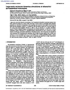
To compare the velocity and position Verlet integrators of Eqs. (2.17) and (2.22), respectively, we choose a pure Lennard-Jones ( 12-6) fluidFith 864 particles. The reduced temperature of the system is T = 2.0 and the reduced density is po 3 = 1.0. The potential is cutoff at r, = 3~. The comparison is made by studying the energy conservation as a function of time step At for a run whose real time is NAt. This energy conservation is defined to be A& At) = -$ $,
/ E(kA;(;
=(‘)
/.
(2.23)
A value of NAt = 1.0 is chosen and kept the same for all runs. Thus for the two integrators, we solve the classical equations of motion and measure the energy conservation as a gnction of time step. In Fig. 1, we plot the dependence of hE on At for the two integrators. The result is very interesting. The curve shows that the velocity Verlet integrator is better at small time steps, but that it becomes unstable more quickly than the position Verlet integrator. For energy conservation tolerances acceptable for typical molecular dynamics calculations, it seems that the velocity Verlet integrator is superior. However, for stability at large time steps, the position Verlet seems better and would thus be a suitable integrator for hybrid Monte Carlo calculations.
C. Reversible algorithms factorizations
based on generalized
Trotter
It is well known that the Trotter factorization can be generalized to a sum of operators. If the Liouvillian takes the form iL = i
iL,
k=l
then the propagator can be expressed as
(2.24)
2 “M 2
-4.5
-5.0
-5.5
0
3 At(x103
4
‘5
6
)
FIG. 1. Comparison of the energy conservation dependence on time step as given by Eq. (2.1) for the velocity Verlet (dashed line) and position Verlet (bold line) integrators for the LJ( 12-6) potential.
e
if3 _-
[“ii’ uk(At/z)] u,,(At) k=l n-l : ,& U,,-,(At/2) ‘+~(t3/P2),
i
II 1
(2.25)
where U, (h) = eiLkhand At = t/P. Let us define n-l l-J U,(At/2) U,(At) k=l
n-l k& U,,-,(ht/2) .
1
(2.26)
It is a simple matter to show that G( At) gives rise to a reversible algorithm given that for each U, (At) Ut, (At) = U, ‘(At)
= U, ( - At)
(i.e., each L, isHermitian). Thus G(At)G( G( At) generates reversible dynamics.
(2.27) - At) = 1, and
Ill. REVERSIBLE REFERENCE SYSTEM PROPAGATOR ALGORITHM (RESPA) FOR SYSTEMS WITH SHORT AND LONG RANGE FORCES We have previously introduced RESPA3,” for accelerating the integration of the equations of motion for systems with forces, F(x), that can be decomposed into short, F, (x) , and long range forces Fl (x) according to F(x) =F;(x)
+F,(x).
(3.1)
The short range force then determines the time step St. In standard methods the full force must be recomputed at the end of each time step. In the RESPA method, however, the short range force is computed after each time step and the long range force is computed every n time steps. This reduces the number of forces calculated and thereby reduces the CPU time. The decomposition of the forces is accomplished by introducing a switching function S(x) that switches from
J. Chem. Phys., Vol. 97, No. 3,1 August 1992
Tuckerman, Berne, and Martyna: Reversible multiple time scale MD
1 to 0 at some interatomic distance chosen to minimize the CPU time. Then F(x) = S(xV’Cc)
+ [ 1 -S(x)
l.F(x)
(3.2)
1993
Ar;x(O),i(O)
x(At)
=x,
k(At)
=.ks At;x(O),i(O)
and we make the identification ++F,[x(At)]
F, (xl = WV’(x), F,(x) = [ 1 -S(x)]F(x).
(3.3)
In our original formulation we took the reference system to be the dynamical system with only short range forces F,(x). This was solved numerically for n time steps St~ht /n. The equations of motion for the deviations of the reference system from the real system was then solved only once for the time step At. This algorithm is not reversible in time. The Trotter factorization allows us to make this strategy reversible. The basic idea is to define the short range force F, (x) as a reference system force and to rewrite the Liouville operator as iL =i-$+Fs(x)
=iL,
a+Fl(x) JP
?JP
+F,(x)a. aP
The propagator eiLArcan now be factorized as, Gls, (A0 = e
(At/Z)F,(x)d/dpeiL~te(A~/Z)F,(x)d/dp
(3.5)
The middle propagator generates motion using the short range forces. Using the Trotter factorization (6r/2)F,(x)d/dped,d/d~e(dt/2)F,oa/d~ eiL& = [e
1n ,
where St = At/n and n is chosen to guarantee stable dynamics. This gives a good approximation to the middle propagator. The propagators on each end of Eq. (3.5) involve the slowly varying long range force and thus will be well approximated as shown with large time step At = nSt. These factorizations give the overall propagator G,,, (At) = e
(Ar/Z)F,(x)d/dp
Xedr*d/dxe(dl/2)F.(x)d/dp
(df/Z)F,(x)d/dp [e
1
ne(Af/2)F,Wd/dp
(3.7) Examination of Eq. (3.7) reveals that because the long range force propogators correct only the velocities, the long range force as well as the short range force from the previous step carry over as input to the next step. Thus one long range force evaluation and n short range force evaluations will be required in a large time step At. There is therefore no more work required for this reversible propogator than for the corresponding nonreversible RESPA method previously introduced.3 When applied to the initial state {x(O),p(O)}, this propagator generates the solution (expressed in terms of positions and velocities)
(3.8)
In these equations x,{h~x(O),k(O) + (At/2m)F, [x(O)]} and .ic,CAt;x(O),i(O) + (At /2m)I;; [x(O)]} denote the solutions of the short range force subject to the initial conditions{x(O),f(O) + (At/2m)F~[x(O)]}.Thefullfactorization above dictates that x, and jc, are to be determined numerically using the velocity Verlet integrator [see Eq. (2.17) ] iteratively for n small time steps of size St subject to the initial conditions {x(O),k(O) + (At/2m)Fl[x(0)]}. The factorization in Eq. (3.7) is implemented as follows: (a) Starting with the initial state {x(O),p(O)} generate the motion using the propagator ecAt’2’F”dp. This gives the
state{x(OLpW + (At/2)F,[x(O) I}. (b) Using the final state of step (a) as the initial state, generate the motion using the middle propagator in Eq. (3.7). This is equivalent to using the velocity Verlet integrator iteratively n times on the system with only short range forces Fs. (c) Starting with state generated in (b) as the initial state, generate the motion using e(Ar’2)F”dp. This gives the final state Eq. (2.11). In Appendix A, we show to convert this scheme to one which is based on standard Verlet. In Appendix B, we show a few lines of FORTRAN code to illustrate how the algorithm of Eq. ( 3.8 ) is implemented in a typical program. The same treatment can be applied to the factorization given by Eq. (3.8) Gs,s
(3.6)
.
(At)
=
eiL~(At/2)eArF~/d~eiL*(Ar/2),
(3.9) but we shall not do so here because it leads to more computational effort in calculating the potential energy at each step than does the previous factorization. In addition, the position Verlet integrator Eq. (2.22) could have been used in place of the velocity Verlet integrator. Thus there are eight possible factorizations, of which we only discuss one. A system with long and short range forces. To compare reversible RESPA with nonreversible RESPA, we look at a system studied in our previous work.3 The system is a LJ( 12-6) fluid with a cutoff at r, = 3a in,a box containing 864 particles at a reduced temperature T= 1.0 and a reduced density PCY3 = 0.8. For the nonreversible RESPA as outlined in Ref. 3, we study only the reference systems given in Eq. (2.2) of Ref. 3. That is, we let the reference force be simply F, (x) . In all comparisons, we make use of switching function discussed in our previous publications,3s’2 with an inner cutoff of 1.90. For reversible RESPA, we use the integration scheme of Eq. (3.8). These two methods are compared with each other and with ordinary velocity Verlet. We study the dependence of energy conservation on At according to Eq. (2.1) using NAt = 1.0 for all runs. St is fixed at 1.0~ 10 - 3. In Fig. 2 we show the plot of A2 vs At for the three integration methods. We note that reversibleRESPA
J. Chem. Phys., Vol. 97, No. 3,i August 1992
1994
Tuckerman, Beme, and Martyna: Reversible multiple time scale MD -4.0
1
,-_-------- -- -~
I
I
I
-4.5 .---
_a--
*_-I
time. As we shall see below these methods are not analytically reversible. The Trotter factorization of the propagator allows us to make this strategy reversible and higher order in time.
I
*clock), “d.al -. -A rnenibla RESPA _---
_/---
/-
e-’
A. Disparate mass systems -5.0 2 xl 0
-5.5
-6.0
_/--
_H--
&
Consider the case where the degrees of freedom of the system can be subdivided into fast and slow degrees of freedom labeled x and y, respectively. An example is2 that of a binary mixture in which one of the components consists of heavy particles (they subsystem) and the other component consists of light particles (the x subsystem). Then we can decompose the Liouvillian as
.--
_/--
r Y
iL = iL, + iL,, -6.5 1
I
1
2
3
I
4 At(x103
I
1
5
6
7
a ax
)
iL, =i---+F&,y)
FIG. 2. Comparison of the energy conservation dependence on time step as given by Eq. (2.1) for straightforward velocity Verlet (dashed line), nonreversible RESPA (double dashed line), and reversible RESPA of Eq. (3.7) (bold line) for the long range force breakup.
IV. REVERSIBLE REFERENCE SYSTEM PROPAGATOR ALGORITHM FOR SYSTEMS WITH MULTIPLE TIME SCALES We have previously introduced methods for accelerating the integration of the equations of motion for systems with two or more time scales.‘,’ Examples are systems consisting of high frequency oscillators coupled to low frequency oscillators or slow baths,’ and systems consisting of massive (slow moving) particles interacting with light (fast moving) particles, the so-called disparate mass problem.2 These methods are based on defining a reference system for the “fast subsystem,” solving this either analytically or numerically for a sequence of small time steps, deriving equations of motions for the deviations from the exact trajectory, and then solving the equations of motion for this deviation and for the slow degrees of freedom numerically using a much larger time step. When the reference system is solved numerically the method is called RESPA (reference system propagator algorithm), whereas when it is solved analytically the method is called NAPA (numerical analytical propagator algorithm). These methods reduce the number of forces that must be calculated and thus reduce the CPU
a ah
-,
(4.2)
iL, =ja+Fy(xy) d. aY ah The propagator can thus be factorized as Gxyx
and nonreversible RESPA agree well at small time steps, but that reversible RESPA is more stable at large time steps. This is to be contrasted with velocity Verlet for which the energy conservation degrades rapidly at large time steps. To quantify this, iz we wanted to conserve energy to within a tolerance of AE = 5 X 10 - 6, we see from the figure that a time step of 2 X 10 - 3 would be required for velocity Verlet, while nonreversible RESPA would use a time step of 6 X 10 - ’ with n = 6, and for reversible RESPA, a time step larger than 8 X 10 - 3 with n around 8 could be used. From our previous work on long range forces,3 we predict that the CPU savings would be a factor of roughly 3 for nonreversible RESPA and around 4 for reversible RESPA.
(4.1)
where
(At)
=
(4.3)
ei~~(A’/2)ei~P’eiL~(A?/2~.
(4.4) For this GX,,Xfactorization the end propagators involve the fast motion whereas the middle propagator involves the slow motion. Although is it not as obvious as in the long range force case [ Eq. (3.7) 1, these factorization involves the same number of force evaluations as does the nonreversible disparate mass RESPA method previously introduced.2 This follows from the fact that FXY = - Fyx, so that this part of the force need only be calculated while advancing the fast coordinate. The fast propagator can be further factorized e
iL,(At/Z)
=
(s1/2)F~/ap,~s~~aaa~~(6f/2)F~/ap, nn [e
1 9
(4.5)
where St = At/n. The middle propagator in GX,,Xcan also be factorized, but because it involves only the slow motion we can use ei=Ar =
e(ht/2,F~/aP~eArLa/ayecar/2)F~/ap,
(4.6)
If these factorizations are used in Eq. (4.4) the fast degrees of freedom and their conjugate momenta {x,p,) are to be determined numerically using the velocity Verlet integrator [see Eq. (2.17) ] iteratively for n small time steps St subject to whatever the initial conditions might be, whereas the slow degrees of freedom are to be determined using the velocity Verlet integrator for only one large step At. We can summarize the numerical procedure that follows from application of GXYXas follows: (a) Use the velocity Verlet integrator for n/2 time steps St = At /n to generate the state at time At /2 under the action of the the propagator eiLxAr” starting from the initial state {x(0)s(O),pX (O),pu(O)}. Note that during this step &p,} is unchanged. (b) Use the velocity Verlet integrator for one time step At to advance the system from the final state of step (a) using the slow propagator Eq. (4.6). (c) Use the velocity Verlet integrator for n/2 time steps
J. Chem. Phys., Vol. 97, No. 3,l August 1992
Tuckerman, Berne, and Martyna: Reversible multiple time scale MD -3.5 ,-
6t = At/n to generate the state at time At /2 under the action of the propagator eiLPrn , starting from the final state in (b). Note that during this step fj,pY} is again held fixed. The resulting state is F( At). In the foregoing the forces on the slow coordinates are recalculated only once every time step, At = n&. If the dimensionality of the fast subsystem is small compared to the dimensionality of the whole system, the forces on the slow coordinates will thus be calculated much less frequently than would be required in the standard methods. There are many variations on the above theme. For example, we could have adopted the Trotter factorization
At ;xo A0 PYO 3 > ( 2 At i( At) = i:, 30 20 aY0 9 > ( 2 x(At)
I “cloclt, RmpA
~
m.eralble
=v,[k;yUWUko],
i(At)
=Y,[WUW(OL~~],
//
5zo= ir
[
-$
;xmf(oLY(o)]
-$x(0),*(0)9(0)]
,-
/-
/’
/’
,/
/’
,/’
/-
,.I’
,/
0.
,/
,I’
/.’
/
-5.5
A
--fi-. 0 0.5
1.0
2.0 1.5 At(xl0’ )
2.5
3.0
FIG. 3. Comparison of the energy conservation dependence on time step as given by Eq. (2.1) for straightforward velocity Verlet (double dashed line), nonreversible RESPA (dashed line), and the disparate mass breakup of Eq. (4.4) (bold line).
versible RESPA is consistently better than velocity Verlet, reversible RESPA is dramatically better and remains remarkably stable even at large time steps. While velocity Verlet becomes unstable at At = 0.04, the energy conservation for reversible RESPA is better than 10 - 5, and for nonreversible RESPA it is better than 5 x 10 - 5. In Fig. 4, we plot the
,^ 2 0 x ‘3 aP
a
I
0 I 2
I 4
I 6
I 6
10
I 12
, 2
I 4
I 6
I 6
I 10
I 12
(4.8) -2 11 0
[
I
FSSPA
,**-
-5.0
0
where x0 =x,
I
“ar,e,
-4.5 5 “M 2
=x,
y(At)
I
-------------_--_
-4.0 / -
Gyxy =ei~,(Ar/2)eiLpfeiL,(Az/Z)
(4.7) and then applied the velocity Verlet breakups. Alternatively, we could use the position Verlet integrator instead of the velocity Verlet factorizations of the different factors in GXYX or Gy.ry.There are eight possibilities in all. For the purposes of the subsequent discussion, we look only at GX,,Xwith the velocity Verlet [see Eq. (2.17) ] breakup applied to each of the factors in GX,,X. Numerical comparison for the disparate mass system. The comparison of reversible RESPA to nonreversible RESPA proceeds now on a system studied in our previous work.2 Again, we look at a sysf\em of LJ( 12-6) particles this time at reduced temperature T = 0.67 and reduced density pa 3 = 0.86, which correspond to the triple point. Again, the potential is cutoff at r, = 3~. The system is comprised of a mixture of 40 light (m = 1) particles and 824 heavy (M = 100) particles. The nonreversible RESPA simulations are carried out as described in Ref. 2 in which the reference force is taken to be Fr (x) = FX [x,y( 0) 1, whereas the reversible RESPA simulations are done using the propagator of Eq. (4.4). When this propagator is used the explicit algorithm for advancing the positions and velocities is given by
1995
t
, )
(4.9)
x, and y, refer to the evolution ofx and y under the actions of ei=*r and ei=Y(,respectively. The velocity Verlet breakup of Eq. (2.17) is applied to the propagators eiLXrand eiL9. In all simulations, the light (x) particles are integrated using 6t = At / 10. The eneri-y conservation is measured as before using Eq. (2.1) an> T is chosen equal to 1.0. In Fig. 3, we show the plot of AE vs At. Figure 3 shows that while nonre-
FIG. 4. (a) The instantaneous fluctuations of the energy about E(0) for velocity Verlet in the disparate mass system at a time step At = 2~ lo-‘. (b) The same except for nonreversible RESPA. (c) The same except for reversible RESPA.
J. Chem. Phys., Vol. 97, No. 3, 1 August 1992
IQ96
Tuckerman, Berne, and Martyna: Reversible multiple time scale MD
instantaneous fluctuations of the energy about the initial value. That is, we plot AE(Q = E(t) -E(O) (4.10) E(O) for each of the three integrators for a time step of At = 2 X 10 - *. In Fig. 3, this corresponds to an average energy conservation of about 3 x 10 - ’ for velocity Verlet, 1 X 10 - 5 for nonreversible RESPA, and 3 x 10 - 6 for reversible RESPA. From these plots, we can determine the maximum of the fluctuations, and discern whether or not the system has a systematic drift. Although the behavior of the instantaneous fluctuations is different in each of the three cases,we see that they are all stable at this time step. B. A stiff oscillator
d aPX 1 a+Ld+F,(x,y) JP, av
+m,Y
-%
JPY
(4.11)
where&y) = F, (X,-Y) - F.,(x). f contains forces on x due to the solvent atoms. This allows us to subdivide the Liouvillian into parts iL, =is+F,(x)
-!JPX
(4.12)
and
iL, =B$j+FyW) ~+~(x,JJ) JPY
tAtj
=
(u/2)
pajay
e(Ar/2)
flwa/ap, (4.17)
Using this factorization of the propagator, the integration procedure generated in terms of positions and velocities is At;x(O),k(O)
+ $0,
At;x(O),f(o) +$(o)
I
I
,
+$(At)
,
eiL~(At/2)eiLPt@iL~(d’R’
= e~,,cAt/2)e’LP’e’L”At/Z).
v(At)
=y(O)
L(At) =j(O)
At2 F y (0), + A@(O)+2m
+&
[Fy(0) + F,(At)].
(4.18)
This particular factorization has the obvious simplicity that the solvent is integrated using velocity Verlet. This breakup is a generalization of the Trotter form as discussed in Sec. II C. The same treatment can be applied to the factorization given by Eq. (4.15) but we shall not do so here. Numerical comparisons for a sti#oscillator in a soft& id. The comparison between reversible and nonreversible RESPA proceeds, as before, on a system considered in our previous work.’ We look at a system of 62 LJ( 12-6) particles in which is imbedded a high frequency harmonic oscillat,“r. The reduced temperature and density of the liquid are T = 2.5 and pa 3 = 1.05. The frequency of the oscillator is taken to be w = 300. Since the peak of the spectral density of the neat liquid at this density and temperature is around w = 20, the oscillator frequency w = 300 is an extremely high frequency. Since the reference force F, (x) = - mw22 is harmonic, we can evaluate the action of the reference system propagator analytically in the usual way as iL,At
x = x cos oAt + * sin @At,
iL&
x = 2 cos wht - wx sin wht.
(4.13)
-% ap,
e
(4.14)
or G,(At)
iLpte
a/ap, e (Ac/z))a,ay
Xe (at/z) qda/ap,
e
The propagator eiLA*can now be factorized as Gy,
Xe
aey e (A~/~)Ax.Y)
dissolved in a soft liquid
Another kind of system of interest is that of a stiff oscillator with vibrational coordinate labeled x buried in a soft bath with coordinates labeled y. For convenience we will also consider the center of mass coordinate of the oscillator as well as its orientational coordinates as part of the bath. It is possible to break the force F, (xg) on the vibrational degree of freedom into a strong, possibly analytically solvable force, and a weak correction. The basic idea is to define a reference system force F,(x) and to rewrite the Liouville operator as iL =k-$-+F,,(x)
G( At) = e (Ar/Z) F+sf
(4.15)
Factorization of the middle propagator in Eq. (4.14) as iL$r = [e (b~/z)F~/ap~~g~jd,a~~(~f~)F?/ap, e (4.16) I”9 where 6t = At/n. If the reference system can be solved analytically (e.g., a harmonic, cubic, or Morse oscillator) then the above factorization is not necessary. A simple way to include the solvent effects into the full propagator yields the following result for GY,.,,(At) :
.
(4.19)
We follow the evolution of the system for 500 periods of the oscillator using ordinary velocity Verlet, NAPA, and reversible NAPA. The result of the comparison of the three integrators is shown in Fig. 5 in which is plotted the energy conservation vs At as in Eq. (2.1) . We see that the reversible NAPA as given by Eq. (4.18) is highly accurate at all time steps, while the nonreversible NAPA tends to become significantly less accurate than reversible NAPA for time steps greater than about 10 - 3. This is due to the fact that nonreversible NAPA, being less stable than reversible NAPA. However, since both NAPA methods are based on analytically solvable stiff reference systems we expect them to agree well at smaller time steps, which they do. The extreme stiffness of the reference system illustrates the advantage of using a reference system algorithm over ordinary velocity Verlet
J. Chem. Phys., Vol. 97, No. 3.1 August IQ92
Tuckerman, Berne, and Martyna: Reversible multiple time scale MD
_.. /’
C
1997
The middle propagator in Eq. (5.2) involves the fast degrees of freedom and the short range forces acting on them and can thus be further factorized as in Eq. (4.5), whereas the middle propagator in Eq. (5.3) involves the slow degrees of freedom propagating under the short range forces and can thus be factorized as in Eq. (4.6). The overall propagator then generates a reversible double RESPA algorithm which can lead to enormous savings in CPU times. The extension of this idea to the stiff oscillator problem is straightforward. VI. REVERSIBLE ALGORITHMS FROM PREDICTORCORRECTORINTEGRATORS
-5.0
0
I
I
I
I
I
I
2
4
6
8
10
12
At(xlO+
14
)
FIG. 5. Comparison of the energy conservation dependence on time step as given by Eq. (2.1) for straightforward velocity Verlet (double dashed line), nonreversible NAPA (dashed line), and the reversible NAPA scheme of Eq. (4.17) (bold line) for the stiff oscillator dissolved in a soft solvent.
which is significantly less accurate than NAPA or reversible NAPA for reasonable energy conservation tolerances (10-3-10-40rbetter). V. SYSTEMS WITH SEPARATION OF TIME SCALES AND SHORT AND LONG RANGE FORCES In the foregoing we have treated systems in which forces can be subdivided into short and long range components. Reference system methods lead to a considerable saving in CPU time. We have also discussed systems in which there is a large separation in time scales such as stiff oscillators embedded in soft fluids or disparate mass systems. In systems with separation of time scales and with force fields that can be decomposed into short and long range forces it is possible to devise reference system methods that can accelerate the solution of the equations of motion. In a previous publication we were able to apply a double reference system approach (double RESPA) to greatly accelerate such systems. This method was not reversible. Here we show how one can generate reversible multiple RESPA procedures to handle systems like these. The propagator for the disparate mass system given in Eq. (4.4) can be expressed as
G,,, (At) = GI;’
(5.1)
where Gi$(At)
= e (Af/2)F,(x.~)a/aP~~iL~f Xe
(Ar/2)F,,kYv)a/ap,
(5.2)
and G$‘(At)
= e (At/2)F~(~y)a/aP~~iL,~t Xe
(At/2vy,w)a/apy
(5.3)
The use of the Liouville operator formalism to derive integrators is a somewhat novel approach. It is, however, satisfying to know that even the standard integrators of molecular dynamics can be obtained from a “first principles” approach. Nevertheless, it is useful to draw the connection between the Liouville operator formalism and the more conventional predictor-corrector scheme.8S’3In this section we address this issue. The usual approach in a predictor-corrector scheme is to “predict” the state of the system based on the initial conditions for the current time step, and then to correct the prediction based on the forces evaluated at the predicted positions. We show that the Trotter breakup ofthe propagator is equivalent to a predictor-corrector scheme. Consider the Trotter breakup of Eq. (2.15) which yields the velocity Verlet eiLAf
=
e(At/2)F(x)a/apeArjia/ax~(A2/2)F(x)a/ap
(6.1) Mathematically, this breakup is equivalent to the following set of equations $=iF(x),
(6.2)
dx dt = v,
(6.3)
$=
(6.4)
+F(x),
with the prescription that Eq. (6.2) is solved for a half time step At /2, with initial conditions {x(O), v(O)} and holding This fixed. the yields predicted value x(O) v(At/2) = v(0) + (At/2m)F(x).ThenEq. (6.3) issolved for a full time step using the predicted value of v and x( 0) as the initial conditions. This yields the true position x(At). Finally, we correct the velocities using Eq. (6.4) with initial conditions x( At) and v( At /2). Following this procedure will yield the scheme of Eq. (2.18). Reversibility comes from having a symmetric set of equations. The middle step in which x is integrated can be thought of as a reference system integration done analytically, since eA*‘a’ax would be the propagator for a reference system with F, (x) = 0. With this in mind, we can easily extend this idea to reversible RESPA. Now consider the example of a system with long and short range force components. The Trotter expansion of the propagator takes the form given in Eq. (3.7) @At
=
e(ACn)Fl(X)a/aP=iLpre(ht/2)Fl(x,a/aP
J. Chem. Phys., Vol. 97, No. 3,i August 1992
,
Tuckerman, Berne, and Martyna: Reversible multiple time scale MD
1998
where iL, = ka /ax + Fs (x>a/ap. this into the equivalent form
As above we can cast
$=+F,(x),
(6.5)
dX
Here we have chosen to use the variable ~7= 1’s dt instead of c as introduced by Hoover in order to make the equation for 7 second order. In order to derive a reversible integrator for the NoseHoover equations, we recognize that these equations can be derived using the Liouville operator”
dt=vs
dv -=LF,(x), (6.6) dt m dv -=-l-F,(x). (6.7) dt m The scheme is now transparent. Eq. (6.5) is integrated for a half step At /2 with initial conditions x (0), v( 0). This yields the predicted value v(At/2) = v(0) + (At/2m)F,(O). Then Eqs. (6.6) are integrated for a full step At using the predicted value v(At /2) and x(O) as initial conditions. This yields a reference system trajectory in which the position is the true position x, (At) = x(At). Then the reference velocity is corrected by Eq. (6.7) using as initial conditions x( At) and v( At /2). As before, reversibility comes from having a symmetric set of equations. It should now be clear how to generate predictor-corrector schemes for other systems with reference forces. VII. A REVERSIBLE ALGORITHM FOR NOSk DYNAMICS We now discuss integration of systems with multiple time scales obeying Nose dynamics.‘4P’5 Recall that Nose’s equations of motion for a system of N particles in virtual variables can be generated from the Hamiltonian
H=E$
pf + V(x) +%+
(3Nf
l)krlns.
(7.1)
iL=zi$+F,.(x)a+f(x)d ap -+&+&+F,(p) ap
ap d, a&
a7
where F,,(p) = Z(p2/m) - 3NkT or F,,(i) = Z(m5z2) - 3NkT. We have introduced the reference system force F,. (x) and the deviation of the true force from the reference force f(x) = F(x) - F,(x). It should be noted that although the conserved energy is I!-+
H’=x
v(x) +&+
(3N+
l)kTvt
(7.5)
as can be verified by computing iLH’ using Eqs. (7.4) and (7.5), this energy is not a Hamiltonian, and the Liouville operator of Eq. (7.4) cannot be derived from it. However, it can be used in conjunction with Eq. (2.1) to measure how well the integration algorithm conserves the energy. Definpropagator as ing reference system the iL, = S/ax + F,(x)a/ap, the propagator eiU* is factorized as G(At) = e (Af/2)
F,wm,
e (At/4)flx)
X,cAt/4~fcx~a/apecAr/2~
a/ap ia/*
e
-
(~t/2)
*pa/ap
efLPr
The equations of motion derived from this Hamiltonian are Xec~t/2~f7a/*e
+--H-
1~ Xe
ap -X7 p=
av .--$-...
-==aH
. aH s=-.--=-, ap,
W-e act with [SJJj,p(Oj
(AZ)
Then, we compute the velocity x(0) from f(O) = x’(St)
(AU~)+~C,VJ)~,~
- St) - (Ar2)Ast) F, [x(O)]
and x’(St) =2x(O)
-
=e
(Al)
In standard Verlet, we start with the initial conditions {x(0),x( -St)), where St=At/n. Using the condition in Eq. (2.20), the standard V er 1et SCh eme is obtained as follows: First, define x’( -St)
v(At) - vI( - At)
VX(i) = VX(i) + 0.5*dt-short
*FX-short(i)
VY(i) = VY( i) + 0.5*dt-short
*FY-short(i)
m(i)
*FZ-short(i)
= VZ(i) + 0.5*dt-short
ENDDO ENDDO CALL FORCEs_Zong
J. Chem. Phys., Vol. 97, No. 3, 1 August 1992
Tuckerman, Berne, and Martyna: Reversible multiple time scale MD
DO i = 1,Natoms V.(i)
= VX(i) + 0.5*dt-Zong*FX-long(i)
F’Y(i) = W(i)
+ 0.5*dt-Zong*FY-long(i)
n(i)
+ 0.5*dt-Zong*FaZong(i)
= vZ(i)
ENDDO (Bl)
In the above, the first loop uses the long range forces from the previous step to obtain the initial conditions on the velocities for the current step. The middle loop runs over the number of inner time steps and computes the reference system positions and velocities from the short range forces. The final loop corrects the velocities from the current values of the long range force. The routines FORCES-short and FORCES-Zong are assumed to update the short and long range components of the force, respectively, dt-short dt 2-short and = dt- Zong/FLO-4 T( Ninner), = (dtwshort)2.
2001
’M. E. Tuckerman, G. J. Martyna, and B. J. Beme, J. Chem. Phys. 93, 1287 (1990). ’ M. E. Tuckerman, B. J. Berne, and A. Rossi, J. Chea Phys. 94, 1465 (1990). ’ M. E. Tucker-man and B. J. Beme, J. Chem. Phys. 94,681l ( 1991). ‘S. Duane, A. D. Kennedy, B. J. Pendleton, and D. Roweth, Phys. Lett. B 195,216 (1987). ‘M. Creutz and A. Goksch, Phys. Rev. Lett. 63,9 ( 1989). ‘H. De Raedt and B. De Raedt, Phys. Rev. A 28,3575 (1983). ‘M. Takahashi and M. Imada, J. Phys. Sot. Jpn. 53, 3765 (1984). aC. W. Gear, NumericalInitial ValueProblemsin Ordinay Dtrerential Equations (Prentice-Hall, Englewood Cliffs, 197 1) . 9 H. F. Trotter, Proc. Am. Math Sot. 10, 545 (1959). “W C Swope H. C. Andersen, P. H. Berens, and K. R. Wilson, J. Chem. Phys: 76,63+ ( 1982). “J. C. Sexton and D. H. Weingarten, Nucl. Phys. B (in press); Nucl. Phys. B Proc. Suppl. 26,613 (1992). “M. E. Tuckerman and B. J. Beme, J. Chem. Phys. 95,8362 (1991). I3 M. P. Allen and D. J. Tildesley, ComputerSimulation ofLiquids (Oxford University, Oxford 1989). 14S.Nest, Mol. Phys. 52, 255 (1984). Is S. No&, J. Chem. Phys. 81,5 11 ( 1984). 16W. G. Hoover, Phys. Rev. A 31, 1695 (1985). “D. J. Evans and G. P. Morriss, Statistical Mechanics of Nonequilibrium Liquids (Academic, San Diego, 1990). I’M. E. Tuckerman and B. J. Beme, J. Chem. Phys. 9.5,4389 (1991).
J. Chem. Phys., Vol. 97, No. 3,1 August 1992