Georgia Institute of Technology, Atlanta, GA, USA. ..... the relationship of this formulation to Gibbs-Appell's .... of the matrix setting of Gibbs-Appell equations. The.
Review of Classical Approaches for Constraint Enforcement in Multibody Systems ∗ Andr´e Laulusa, SIMUDEC Pte Ltd, Singapore Science Park II, Singapore 117628, and Olivier A. Bauchau Daniel Guggenheim School of Aerospace Engineering, Georgia Institute of Technology, Atlanta, GA, USA.
Abstract
1
A hallmark of multibody dynamics is that most formulations involve a number of constraints. Typically, when redundant generalized coordinates are used, equations of motion are simpler to derive but constraint equations are present. While the dynamic behavior of constrained systems is well understood, the numerical solution of the resulting equations, potentially of differential-algebraic nature, remains problematic. Many different approaches have been proposed over the years, all presenting advantages and drawbacks: the sheer number and variety of methods that have been proposed indicate the difficulty of the problem. A cursory survey of the literature reveals that the various methods fall within broad categories sharing common theoretical foundations. This paper summarizes the theoretical foundations to the enforcement in constraints in multibody dynamics problems. Next, methods based on the use of Lagrange’s equation of the first kind, which are index-3 differential algebraic equations in the presence of holonomic constraints, are reviewed. Methods leading to a minimum set of equations are discussed; in view of the numerical difficulties associated with index-3 approaches, reduction to a minimum set is often performed, leading to a number of practical algorithms using methods developed for ordinary differential equations. The goal of this paper is to review the features of these methods, assess their accuracy and efficiency, underline the relationship among the methods, and recommend approaches that seem to perform better than others. Keywords: Constrained multibody dynamics; Constraint conditions; Numerical methods; Differential/Algebraic equations.
Introduction
Multibody systems are characterized by two distinguishing features: system components undergo finite relative rotations and these components are connected by mechanical joints that impose restrictions on their relative motion. Finite rotations introduce geometric nonlinearities, hence, multibody systems are inherently nonlinear. Mechanical joints result in algebraic constraints leading to a set of governing equations that combines differential and algebraic equations. A survey paper by Schiehlen [1] summarized different approaches to the derivation of the equations of motion for multibody systems. The choice of various frames of reference, system variables and mechanics principles were reviewed. While the dynamic behavior of the system is, of course, independent of the formalism used to describe it, the form of the equations of motion and the amount of effort required to derive them is affected by all these choices. The same remarks apply to the various methods used to enforce constraint conditions: the effort involved in the derivation of the complete system of governing equations and associated constraints, as well as the computational cost required for their solution and the resulting accuracy all critically depend on the theoretical formalism and numerical methods used to solve the problem. The goal of this review paper is to contrast the features of the various approaches used to enforce constraints in multibody systems, assess their accuracy and efficiency, underline the relationship among the methods, and recommend approaches that seem to perform better than others. Consider a multibody system described by n generalized coordinates, q, and m constraints that could be a mixture of holonomic and nonholonomic constraints. ∗ Journal of Computational and Nonlinear Dynamics, 3(1), The classical formulation of the problem leads to Lapp 011004 1-8, 2008. grange’s equations of the first kind; as discussed in sec1
tion 2.1, this approach involves m Lagrange’s multipliers. Next, several approaches that eliminate these multipliers are reviewed and compared: Maggi’s, the index-1, the null space, and Udwadia and Kalaba’s formulations. The geometric interpretation of the problem presented in section 2.3 presents valuable insight into the behavior of constrained systems. Methods based on the use of Lagrange’s equation of the first kind are discussed in section 3. However, mathematical studies underline the numerical difficulties associated with the solution of these index-3 differential algebraic equations (DAEs), and recommend reduction of the index level as a means of circumventing numerical problems. Section 4 describes numerous procedures to obtain equations involving a minimum set of coordinates, thereby completely eliminating the algebraic nature of the governing equations. Methods developed for the solution of ordinary differential equations (ODEs) are then applicable to the reduced system of equations.
2
relationships among the generalized velocities; it is assumed that these relationships depend on the generalized velocities in a linear fashion (Pfaffian form). On the other hand, some of the constraints could be holonomic; this means that they can be integrated to the form C(q, t) = 0. If all the constraint are holonomic, B(q, t) is called the constraint Jacobian matrix, and the n generalized coordinates, q, are linked by m algebraic constraints. If these latter are independent, it is conceptually possible to partition the generalized coordinate array into independent, q I(n−m) , and dependent coordinates, q D , such that q T = bq IT , q DT c and q D = f (q I ), (m) leading to the elimination of the dependent variables. Unfortunately, this approach is fraught with difficulties: it is not clear which generalized coordinates should be selected to be independent. Furthermore, a poor selection of the independent set of coordinates might render f (q I ) singular, a suitable set of independent coordinates might become unsuitable for different configurations of the system, and finally, function f (q I ) might be so complex as to preclude any practical computations. Lagrange’s equations of the first kind form a set of (n + m) Differential-Algebraic Equations (DAEs) for the (n + m) unknowns, q and λ; indeed, Lagrange’s multipliers are algebraic variables, i.e. no time derivatives of these variables appear in the equations, whereas first and second order derivatives of the generalized coordinates are present, as implied by Newton’s second law. Gear, Petzold and co-workers [2, 3, 4], as well as Brennan [5], have given a formal definition of the index of a system of DAEs. The governing equations for mechanical systems with holonomic constraints are index-3 DAEs; typically, higher indices result in more arduous solution processes. Constraints written in the form of eq. (2) are sometimes called velocity level constraints. A time derivative of these constraints then yields
Theoretical developments
This section reviews three basic aspects of constrained dynamical systems described by n generalized coordinates, q, and m constraints that could be a mixture of holonomic and nonholonomic constraints. The first formulation of the problem gives the equations of motion as Lagrange’s equations of the first kind; this approach involves m Lagrange multipliers. Next, several approaches have been proposed to eliminate Lagrange’s multipliers: among them Maggi’s, and Udwadia and Kalaba’s formulations are reviewed. Finally, the geometric interpretation of the problem is presented.
2.1
Lagrange’s equations of the first kind
Lagrange’s equations of the first kind are generally written in the following form T M(n×n) ¨q (n) + B(n×m) λ(m) = F (n) ,
˙ t) − B(q, ˙ t) q˙ = c (q, q, B(q, t) ¨q = −b(q, ˙ t), (m) the acceleration level constraints.
(1)
2.2
where M = M (q, t) is the symmetric, positive-definite ˙ indicates a derivative with respect to mass matrix, (·) ˙ t) are the dynamic and externally aptime, F = F (q, q, plied forces, λ the array of m Lagrange’s multipliers, and the subscripts indicate the sizes of the corresponding arrays. The constraints applied to the system are written as D(m) = B(m×n) (q, t) q˙ (n) + b(m) (q, t) = 0,
(3)
Algebraic elimination of Lagrange’s multipliers
In this section, algebraic procedures for the solution of Lagrange’s equations of the first kind are presented. In all cases, the approach eliminates Lagrange’s multipliers to obtain a set of ordinary differential equations (ODEs).
(2)
2.2.1
Maggi’s formulation
where B(q, t) is the constraint matrix. Constraints While the original derivation of Maggi’s formulation apcould be nonholonomic, in which case eq. (2) expresses peared in 1896 [6], then again in 1901 [7], it is only 2
in 1972 that it is presented in the English literature by Neimark and Fufaev [8]. More recently, Kurdila et al. [9] and Papastavridis [10] have shown the relevance of this formulation to computational methods for constrained multibody systems. The formulation begins with the definition of a set of (n − m) kinematic characteristics, denoted e, that satisfy the following relationships ¯ ¯ ¯ · ¯ ¸ ¯ 0(m) ¯ ¯ b(m) (q, t) ¯ B(m×n) (q, t) ¯ ¯ ¯= ¯. ˙ ¯ ˇ ¯ e(n−m) ¯ ˇ((n−m)×n) (q, t) q+ B b(n−m) (q, t) ¯ (4) The first m equations of this system represent the constraints, see eq. (2), while the last (n − m) equations define independent kinematic characteristics, which are sometimes called kinematic parameters, generalized speeds or independent quasi-velocities. In general, these quantities cannot be integrated, i.e. no p exists such that p˙ = e. Note that the choice of the kinematic parameters, a crucial part of the procedure, is left to the analyst. The number of dofs of the system is n − m. ˇ defines a linear transThe matrix formed by B and B formation that is assumed to be invertible; this implies a full rank constraint matrix and a judicious choice of the kinematic parameters. The following notation is used · ¸ Bm×n (q, t) Bn×n = (5) ˇ((n−m)×n) (q, t) . B
Lagrange’s multipliers have been eliminated from Maggi’s equations: in view of eq. (8), the term ΓT B T λ vanishes. It is important to note that the choice of kinematic characteristics is not unique. Ignoring, for simplicity, arrays b and ˇb, eq. (7) becomes q˙ = Γe: whereas the generalized velocities, q, ˙ are uniquely defined, any set of linearly independent vectors can be selected to span the null space, Γ, each leading to a new set of kinematic characteristics. Maggi’s formulation consists of eqs. (10) and (7), which form a system of (2n − m), first order ODEs for the (2n − m) unknown, e and q. Maggi’s equations eliminate Lagrange’s multipliers from Lagrange’s equations of the first kind. However, it is possible to compute these multipliers once Maggi’s equations have been solved. Properties (8) imˇ = I, hence, multiplying eq. (1) by Γ ˇ T yields ply that B Γ T ˇ λ = −Γ (M ¨q − F ). Introducing eq. (9) then leads to h i ˇ T M Γ˙e + M Γe ˙ − M d˙ − F . λ = −Γ (11) 2.2.2
Index-1 formulation
Consider the system of equations consisting of the Lagrange’s equations of the first kind, see eq. (1), and the acceleration level constraints, eq. (3), written in a matrix form as · ¸· ¸ · ¸ ¨q F M BT = . (12) c B 0 λ
The inverse of this matrix is denoted £ ¤ −1 ˇ (n×m) (q, t) Γ(n×(n−m)) (q, t) . Bn×n = Γ
This system is now an index-1 set of DAEs, which can (6) be formally solved for the accelerations and Lagrange’s The generalized velocities are now readily expressed in multipliers. This system is equivalent to Lagrange’s equations of the first kind, see eq. (1), if and only if the terms of the kinematic characteristics as initial conditions of the problem satisfy the constraint ˇ b + Γ ˇb) = Γe − d(q, t). q˙ = Γe − (Γ (7) conditions, i.e. C(q 0 , t0 ) = 0 and D(q 0 , q˙ 0 , t0 ) = 0 for holonomic and nonholonomic constraints, respectively, Since eqs. (4) and (7) are inverse of each other, the where q = q(t ) and q˙ = q(t ˙ 0 ) are the initial condi0 0 0 following relationships must be satisfied tions of the problem. · ¸ · ¸ · ¸ ˇ BΓ It is easily shown that system (12) has a unique B £ˇ ¤ BΓ I 0 Γ Γ = = , (8) solution if and only if matrix B is of full rank and ˇ ˇ ˇ ˇ 0 I B B Γ BΓ the mass matrix is invertible, see e.g. Nikravesh [11]. ˇ + ΓB ˇ = I. Matrix Γ plays a central role in the First, Lagrange’s multipliers can be found as λ = and ΓB derivation of Maggi’s equations. The property BΓ = 0 −(BM −1 B T )−1 (c − BM −1 F ), and next, they are inimplies that Γ spans the null space of the constraint ma- troduced in the first equations to yield the accelerations trix ; B and Γ are orthogonal complements. Next, the and the forces of constraint, F c = B T λ, of the system generalized accelerations are expressed in terms of the as ¡ ¢−1 ¡ ¢ kinematic characteristics by taking a time derivative of M ¨q = F + B T BM −1 B T c − BM −1 F , (13a) eq. (7), leading to ¡ ¢−1 ¡ ¢ Fc = −B T BM −1 B T c − BM −1 F . (13b) ˙ ˙ − d. ¨q = Γ˙e + Γe (9) The governing equations of the system can be expressed System (13a) is now a system of second order ODEs, in terms of the kinematic characteristics by introducing which can be solved to predict the dynamic behavior of eq. (9) into eq. (1), and pre-multiplying by ΓT to find the system. These equations have appeared in Hemami and Weimer [12], L¨otstedt et al. [13, 3] and Gear et ˙ ˙ e = ΓT F + ΓT M d. (ΓT M Γ) e˙ + (ΓT M Γ) (10) al. [14]. 3
2.2.3
The null space formulation
derived from D’Alembert’s principle. This formulation is more general than those presented in the previous sections, which require the constraint matrix to be of full rank, whereas the MPGI is unique and always exists. The same authors [26] later presented a simpler derivation of their formulation that bypasses the concepts of generalized inverses. When rank(B) = m, they proved the existence of Lagrange’s multipliers and expressed them in terms of the constraint forces; when rank(B) < m, Lagrange’s multipliers are not unique, although the constraint forces are unique. Udwadia et al. [20] presented an extended form of D’Alembert’s principle that is able to deal with nonholonomic constraints, which might be nonlinear expressions of the generalized velocities. Furthermore, they showed that the previous formulation could be derived without invoking MPGI. The geometric interpretation of the results in terms of projection operators, as presented in section 2.3, appeared in ref. [27] and the relationship of this formulation to Gibbs-Appell’s equations was explored in ref. [28]. Finally, the same authors [29, 30] generalized the formulation to deal with mechanical system involving “non-ideal” constraints, i.e. constraints associated with constraint forces whose virtual work might not vanish. It is interesting to note that the use of Gauss’ principle for the solution of constrained multibody systems was already proposed by Lilov and Lorer [31] in 1982; their approach involves the MPGI of the constraint matrix.
It is also possible to solve system (12) in an expeditious manner with the help of the null space, Γ, introduced in section 2.2.1. Pre-multiplying the first equations by ΓT eliminates Lagrange’s multipliers and yields the null space formulation (NSF) · T ¸ · T ¸ Γ M Γ F ¨q = . (14) B c Here again, this system forms a set of second order ODEs, the solution of which requires B to be of full rank and M to be invertible. A number of authors independently developed this formulation. Hemami and Weimer [12] introduced the orthogonal complement, Γ, of the constraint matrix, B, to obtain eqs. (14) for small-scale systems, although no systematic procedure was proposed to determine Γ. They also demonstrated the equivalence of this approach to Kane’s equations [15, 16]. Garc´ıa de Jal´on et al. [17, 18] also derived eqs. (14). Borri et al. [19] proposed the acceleration projection method, which decomposes the generalized acceleration as ¨q = Γζ + B T η. Substituting this decomposition into eqs. (14) express ζ and η in terms of M, B, ΓT , F and c, leading to second order ODEs. 2.2.4
Udwadia and Kalaba’s formulation
The results presented in the previous section can also be recast in a more compact and general form in terms of Moore-Penrose generalized inverses (MPGI) to yield Udwadia and Kalaba’s formulation (UKF). The term featuring the matrix inverse in eq. (13a) can be written as B T (BM −1 B T )−1 = M 1/2 (BM −1/2 )T [(BM −1/2 )(BM −1/2 )T ]−1 = M 1/2 (BM −1/2 )+ . Eqs. (13a) and (13b) now become ¢ ¡ M ¨q = F + M 1/2 (BM −1/2 )+ c − BM −1 F , (15a) ¡ ¢ −M 1/2 (BM −1/2 )+ c − BM −1 F , (15b) Fc =
2.2.5
Comparison of the ODE formulations
The formulations presented above all transform the (2n + m) first order DAEs associated with Lagrange’s equations of the first kind into ODEs by eliminating Lagrange’s multipliers. Maggi’s formulation, eqs. (10) and (7), yields (2n − m) first order ODEs. On the other hand, the index-1 formulation, eqs. (13a), NSF, eqs. (14), or UKF, eqs. (15a), form sets of n second order ODEs for the n generalized coordinates, which could alternatively be recast as sets of 2n first order ODEs for the n generalized coordinates and n generalized velocities. The first observation is that these methods decrease the size of the problem from (2n + m) for Lagrange’s equations of the first kind to 2n for the index-1 formulation, NSF, or UKF, and (2n − m) for Maggi’s formulation. However, this dimensional reduction comes at a price: the evaluation of the null space of the constraint matrix in Maggi’s and the NSF, or the evaluation of MPGI in UKF. On the other hand, Lagrange’s equations of the first kind are typically formulated in terms of generalized coordinates that will render system ma-
respectively. A process similar to that developed by Udwadia et al. [20] can be used to solve the system formed by eqs. (14) and ΓT F c = 0, to recover eqs. (15a) and (15b). This underlines the close relationship between the present formulation and the NSF of section 2.2.3. Eqs. (15a) and (15b) were first presented by Udwadia and Kalaba [21, 22, 23, 24], based on Gauss’ principle: the explicit equations of motion were expressed as the solution of a quadratic minimization problem subjected to constraint conditions at the acceleration level. In a later paper [25], the same equations were 4
2.3
trices highly sparse, leading to efficient solution techniques, as discussed by Orlandea et al. [32, 33]. Hence, the main advantage of the above techniques is not so much the reduction in the number of equations, but rather the change in their mathematical nature, from DAEs to ODEs.
The geometric interpretation of constraints
Whereas the formulations presented in the previous sections are of a purely algebraic nature, the present section focuses on a more geometric interpretation of constrained dynamical problems, based on the concept of projection operators. This geometric interpretation of the problem has been investigated by a number of authors using similar concepts: Brauchli et al. [35, 36] and Udwadia and Kalaba [27]. Since the mass matrix is a symmetric, positivedefinite matrix, it can be factorized as M = SS T using the Cholesky factorization [37], for instance. Multiplying eq. (1) by S −1 then leads to
The second observation is that Maggi’s formulation enforces velocity level constraints for holonomic constraints, whereas acceleration level constraints are enforced in the other formulations. This fact has important implications for numerical implementations of these approaches: the constraint drift phenomenon will be significantly more pronounced when using the latter formulations than when using Maggi’s formulation. Typically, a constraint violation stabilization technique will be required to compensate for this drift. While the double differentiation of the constraints with respect to time is a widely used practice in multibody dynamics, it has the potential to adversely affect the numerical solution procedure. In fact, Campbell and Leimkuhler [34] studied the effects of differentiation of the constraints in DAEs; they concluded: “Thus, the differentiated system may be less well behaved numerically for a given method than either the original DAEs or an equivalent state-space form for that method. These numerical difficulties can take the form of increased stiffness, extraneous positive eigenvalues, and more stringent step-size restrictions.”
¨ˆq + F ˆc = F ˆ,
(16)
where the scaled accelerations were defined as ¨ˆq = S T ¨q ˆ c = S −1 F c and F ˆ = S −1 F . and the scaled forces as F ˆ = Next, The scaled constraint matrix is defined as E −1 T S B , and finally, the same scaling is applied to the ˆ T ¨ˆq = c. A constraint equation, eq. (3), to yield E ˆE ˆ T E] ˆ −1 E ˆ T , is inscaled projection operator, Pˆk = E[ troduced; the image of this projector is the scaled conˆ and it operates in a space of metric straint matrix, E, Mc = M −1 , i.e. the inverse of the mass matrix. Since ˆ = S −1 B T λ = Eλ, ˆ which shows that F ˆ c belongs to F ˆ it follows, by construction, that the range space of E, ˆc = F ˆ c. Pˆk F
Next, it is important to understand that Maggi’s formulation requires the definition of a set of m kinematic parameters. Since the set of linearly independent vectors spanning the null space is not uniquely defined, the choice of kinematic parameters is not unique and the reduced equations can take a variety of forms. On the other hand, the other formulations do not require the introduction of this new set of variables: they are expressed in terms of the generalized coordinates originally used to describe the system.
(17)
The projection of the scaled accelerations yields Pˆk ¨ˆq = ˆE ˆ T E] ˆ −1 E ˆ T ¨ˆq = E[ ˆE ˆ T E] ˆ −1 c, and finally, E[ ˆ +T c = Pˆk E ˆ +T c, Pˆk ¨ˆq = E
(18)
where the last equality follows from the properties of ˆ + denotes the MPGI of E. ˆ projection operators, and E The scaled equations of motion, eqs. (16), are multiplied by the projector to find ³ ´ ˆ c = Pˆk F ˆ −E ˆ +T c = Pˆk F ˆ −E ˆ +T c , F (19)
The UKF presents a number of advantages over the other formulations. The MPGI appearing in eq. (15a) always exists, whereas the other formulations require a full rank constraint matrix. Hence, UKF is capable of dealing with problems featuring rank deficient constraint matrix, such as those involving redundant constraints. Furthermore, problems with variable number of dofs, such as intermittent contact problems, or problems involving rolling and slipping, are readily treated. In contrast, such situations will be problematic for minimum set approaches, since the number of kinematic parameters must change as the constraints change or become redundant.
where the last equality was obtained with the help of eq. (18). This important relationship shows, again, that constraint forces are entirely contained within the imˆ of the projector, i.e. the constraint forces beage, E, long to the space defined by the scaled constraint matrix. Next the accelerations of the system are computed from eq. (16) as ¨ˆq = Pˆ⊥ F ˆ +E ˆ +T c.
(20)
It is easily shown that eqs. (15a) and (15b) are identical to eqs. (20) and (19), respectively. Clearly, system accelerations have a component in the image of 5
ˆ +T c and a component in the the projector, Pˆk ¨ˆq = E ˆ . The geometric orthogonal subspace, Pˆ⊥ ¨ˆq = Pˆ⊥ F interpretation of these results is illustrated in fig. 1. According to eq. (16), the scaled unconstrained forces, ˆ , are the sum of the scaled constraint forces, F ˆ c , and F the scaled accelerations of the system. The scaled conˆ straint forces are the difference between vectors Pˆk F +T ˆ and E c, both contained in the image of the projector, as implied by eq. (19). On the other hand, system ˆ +T c, contained in accelerations are the sum of vector E ˆ , contained the image of the projector, and vector Pˆ⊥ F in the orthogonal subspace.
Image of the projector = constraint gradient
gent space. These projected Newton equations were then shown to be equivalent to Lagrange’s equations. Generalizing to nonholonomic constraints in Pfaffian form, Ess´en obtained equations of motion in terms of quasi-velocities by projection of Newton’s equations onto Γ. The resulting equations were shown to be general Boltzmann-Hamel equations. The relationship of this approach to Kane’s method was also underlined. Blajer [41, 42] summarized much of the work done within the framework of differential Riemannian geometry: index-1 formulation, NSF, and Maggi’s formulation for combined holonomic and nonholonomic constraints have all been presented in this framework. For holonomic systems, the equivalence of Maggi’s formulation and Boltzmann-Hamel equations was shown, as was the equivalence of the projective formulation and of the matrix setting of Gibbs-Appell equations. The author underlined the need to develop efficient methods for computing the time derivative of the null space, an indispensable ingredient for the application of Maggi’s and projective formulations. He also proposed a technique for the elimination of constraint violations that affect the index-1, null space and Maggi’s formulations. The Boltzmann-Hamel equations are immune from these violations because independent generalized coordinates are introduced.
^ F c ^ F .. ^ q
^^ ^ Fc P2 F ^ +Tc E
^ ^ Pz F Constraint manifold
Figure 1: Geometric representation of constraint dynamics with holonomic constraints. Although appearing as orthogonal projections in this illustration, projections are, in fact, operating in the metric of the inverse of the mass matrix.
2.4
3
Methods solving Lagrange’s equation of the first kind
Orlandea et al. [32, 33] have presented an approach to the dynamic analysis of mechanical systems based on the solution of Lagrange’s equation of the first kind, a system of index-3 DAEs in the presence of holonomic constraints. While the number of generalized coordinates used in this approach is much larger than the minimum set, they argue that the numerical solution of the resulting equations can be efficiently obtained by taking advantage of their sparsity through the use of appropriate algorithms. To overcome the numerical problems associated with the solution of DAEs, numerically dissipative time integrators were used that are specifically designed for stiff problems, see Gear [43], who also clearly underlined the difficulties associated with the solution of DAEs [44]. It is interesting to note that this early approach proposes a purely numerical solution to the challenges posed by Lagrange’s equations of the first kind: stiff integrators are used to deal with DAEs. More recently, a similar approach has gained popularity for multibody system modeled by the finite element method. Gear and coworkers [45, 2] have extensively studied DAEs and concluded in 1984: “If the index does not exceed
Additional formulations
The theoretical developments presented in the above sections are well known, but additional formulations have also been presented in research papers, often of a more theoretical nature. In fact, many papers focus on explaining relationships, and often establishing equivalence, between various formulations rather than proposing practical numerical methods for the enforcement of constraints. For instance, Borri et al. [38] have shown the equivalence of Maggi’s and Kane’s equations [15, 16]. Maißer [39] used Riemannian geometry formalism to study holonomic multibody systems. This work focuses on tree topology systems and emphasizes the generation of the equations of motion within the Riemannian formalism using Christoffel symbols. Coordinate partitioning was suggested as a solution method for the resulting equations. Ess´en [40] considered systems of particles and derived a minimal set of equations of motion for holonomic systems by projecting Newton’s equations onto the tan6
1, automatic codes [...] can solve the problem with no trouble.” Furthermore, “If [...] the index is greater than one, the user should be encouraged to reduce it.” These observations prompted the multibody community to engage along two distinct avenues of research. First, coordinate reduction techniques that eliminate Lagrange’s multipliers all together, reducing the DAEs to ODEs. Second, index reduction techniques that reduce the governing equations of motion to index-1 equations. A survey paper by Haug [46] describes in a conceptual manner these two approaches to computational methods in constrained dynamics; Nikravesh [11] investigated two algorithms representative of those two approaches; the first algorithm reduces the problem to an index-1 system, the second used a coordinate partitioning method based on ref. [47].
4
these methods no longer represent a numerical implementation of Maggi’s formulation; they might be better characterized as “Maggi-like” methods. Kurdila et al. [9] and Papastavridis [10] first pointed out the unifying role of Maggi’s formulation, which forms the basis for many of these coordinate reduction techniques that are equally applicable to holonomic and nonholonomic constraints. They point out that various methods only differ by the choice of the basis selected to span Γ, which in turns, determines the kinematic characteristics; the equations of motion are then projected onto this subspace. Clearly, matrix B and its inverse, as defined by eqs. (5) and (6), respectively, fully characterize Maggi’s formulation. A number of “Maggi-like” formulations only differ by the computational tool used to evaluate Γ. The following approaches have been used: the zero eigenvalue method [48], the coordinate partitioning method based on the LU factorization [47, 49], and the singular value decomposition, (SVD), method [50, 51]. Since these approaches were reviewed by Kurdila et al. [9], details are not repeated here. The following paragraphs discuss methods that were developed after their review paper appeared.
Ordinary differential equation techniques
The challenges posed by the differential algebraic nature of Lagrange’s equations of the first kind can also be dealt with by means of alternative formulations of the equations of motion. This section deals with methods that recast the governing equations in terms of ODEs. A logical approach is to eliminate the redundant generalized coordinates to obtain a minimum set of equations, bypassing the need for constraints; this is the approach followed in Maggi’s formulation. However, it is also possible to obtain ODEs for all the generalized coordinates selected by the user to describe the system.
Amirouche et al. [52] applied the Householder transformation technique to the transpose of the constraint matrix, assumed to be of full rank, to obtain a full rank, upper triangular matrix But(n×m) = HB T , where H(n×n) is the product of successive Householder transformations. The Gram-Schmidt orthonormalization (GSO) process was then used to find an orthonormal basis, D, which was partitioned as D(n×n) = [ D1(n×m) D2(n×(n−m)) ]. The fun4.1 “Maggi-like” formulations damental matrices of Maggi’s formulation are easThe essence of Maggi’s formulation is the construc- ily identified as B T = [ B T H T D ] and B −1 = 2 tion of the null space, Γ of the constraint matrix B, [ H T D1 (BH T D1 )−1 H T D2 ]. The authors pointed which enables the elimination of Lagrange’s multipliers out that their approach, called “recursive Householder through the use of orthogonal complements, BΓ = 0. transformation method,” is equivalent to the zero eigenSince B is a function of time, so must be Γ, and in value [48] and SVD methods [50, 51], while achieving numerical implementations, it must be recomputed at higher computational efficiency. each time step, a considerable computational burden. Hence, the vectors spanning Γ at two different steps Agrawal and Saigal [53] also used the GSO process could be different, resulting in a new set of kinematic to generate a basis of Γ. For holonomic constraints, characteristics at each time step. To overcome these Γ is tangent to the constraint manifold, hence the approblems, many researchers have evaluated Γ at the be- proach was called “tangent coordinate method.” This ginning of the simulation, Γ0 , and kept it constant for approach is very similar to that presented by Liang and the subsequent time steps of the analysis. When us- Lance [54], except that matrix E is also constructed ing this approach, Lagrange’s multipliers are no longer using the GSO process, a method that is faster and eliminated, since B(t)Γ0 6= 0. At regular intervals, Γ requires less computer memory. The process generis recomputed. Typically, a criterion is developed that ates an orthogonal matrix T , which is partitioned as T T T T2(n×(n−m)) identifies the appropriate time step when this expensive T(n×n) = [ T1(n×m) ]. The fundamental operation is to be performed; various criteria have been matrices of Maggi’s formulation are easily identified as used by various researchers. It should be noted that B T = [ B T T2T ] and B−1 = [ T1T (BT1T )−1 T2T ]. 7
4.2
Maggi’s formulations
ponents of the generalized velocity array. In view of ˇ has a eq. (4), this implies that each row of matrix B single nonzero entry. A good choice of this extraction is initially determined by performing a Gaussian triangulation of the constraint matrix with full pivoting: the pivot locations indicate the generalized velocities to be extracted. This choice might become unsuitable during the simulation, when a previously selected pivot becomes very small; a new extraction is then selected. In a subsequent paper, Garc´ıa de Jal´on et al. [17] also use the SVD to identify the kinematic parameters. They concluded that while this approach might yield a set of kinematic parameters that are suitable over a longer period of the motion, it is also more expensive than the extraction approach. Avello et al. [64] further elaborated on the extraction procedure by showing that it leads to a highly parallelizable algorithm. The columns of Γ are each computed in parallel as the solution of an elementary velocity problem, and furthermore, the triple product ΓT M Γ can ˙ apalso be evaluated in parallel. The terms of array Γe pearing in Maggi’s equations are also computed in parallel and correspond to solutions of elementary acceleration problems. For computational efficiency, the overall approach uses recursive techniques for open loop mechanisms; in the presence of closed loops, the augmented Lagrangian formulation is used, see section 3.2.2 of ref. [65].
Wampler et al. [55] devised a simple approach in which Maggi’s kinematic characteristics are selected to be a subset of the generalized speed within the framework of Kane’s method. However, they only presented analytical examples of their procedure. A few authors have developed approaches that update the null space at each time step. Kim and Vanderploeg [56] proposed an updating scheme which maintains the directional continuity of the null space. This approach was reviewed by Kurdila et al. [9], details are not repeated here. The following paragraphs discuss methods that were developed after their review paper appeared. Liang and Lance [54] have used the GSO process to generate independent coordinates that are continuous and differentiable. At first, matrix P(n×n) = T T E(n×(n−m)) ] is constructed, where E T is [ B(n×m) an arbitrary matrix such that P is nonsingular. Typically, E is determined by SVD, or by LU factorization. P is then transformed into an orthogonal matrix V = [ VD VI ] through the GSO process, where VD and VI are of the same dimensions as B T and E T , respectively. The fundamental matrices of Maggi’s formulation are easily identified as BT = [ B T VI ] and B−1 = [ VD (BVD )−1 VI ]. Constraints equations are intimately related to the choice of coordinates used to represent mechanical systems. Garc´ıa de Jal´on et al. developed the concept of “basic coordinates” for constrained rigid bodies; the approach was developed for the kinematic analysis of planar lower-pair mechanisms [57, 58] and later expanded to deal with spatial mechanisms [59, 60]. Serna et al. [61] used this framework to analyze the dynamic response of planar mechanisms. Maggi’s and the NSF were both presented, together with an original approach to the determination of Γ: each column of Γ can be determined by means of the solution of an elementary velocity problem; this is a more physical approach that contrasts with the purely numerical procedures de˙ scribed in the previous sections. Similarly, the term Γe that appears in Maggi’s equations (10) can be evaluated as the solution of elementary acceleration problems. The same approach was used by Garc´ıa de Jal´on et al. [62] who presented a formulation for both open- and closed-loop systems based on natural, or fully Cartesian coordinates. Garc´ıa de Jal´on et al. [63] later showed how “natural coordinates” evolved from the earlier basic coordinates, and used this new concept to describe multibody systems. Γ is determined from eq. (7): q˙ = Γe, because constraints are assumed holonomic and scleronomic. It is then possible to determine Γ corresponding to kinematic characteristics that are an “extraction” of com-
4.3
Discussion of the methods based on Maggi’s formulation
As stated earlier, the vectors spanning Γ are not unique. The methods presented above all define this subspace by different sets of vectors that are obtained by means of different computational processes. Two fundamental criteria can be used to assess the various approaches. First, is the subspace defined by linearly independent vectors? Second, how robust and efficient is the numerical process used to generate this subspace? The first criterion is a necessary condition for the viability of the approach: if the vectors are not linearly independent, Γ is not properly defined. Kurdila et al. [9] pointed out that the approaches of Kane [15] and Wehage and Haug [47] are not robust because they can lead to a poorly conditioned or even singular representations of Γ. To overcome this problem, most other approaches generate an orthogonal basis spanning Γ. The second criterion deals with computational robustness and efficiency. Based on operation count, the computational cost of SVD is known to be two to ten times higher than that of the QR algorithm, depending on the size of the constraint matrix. In turns, the QR algorithm is about two times more costly than the LU 8
factorization. On the other hand, SVD is many times more expensive than the GSO process. However, SVD is probably the most robust algorithm since it can be safely used even when the constraint matrix is not of full rank [50], as is the case in the presence of redundant constraints. Clearly, SVD is the most robust and stable algorithm, but is also the most expensive. An important feature of Maggi’s formulation is that constraints are enforced at the velocity level. Hence, nonholonomic constraints will be satisfied to numerical accuracy, whereas holonomic constraints will drift due to the inherent errors associated with the integration process. However, this drift is minimal, because the kinematic characteristics lie in the hyperplane tangent to the constraint manifold. In fact, Liang and Lance [54] mention that with their approach, “the numerical solution will be satisfactory without any positive constraint violation control or constraint violation stabilization.” This is an important benefit of a rigorous application of Maggi’s formulation. However, the situation is different with the Maggi-like methods that do not update the null space, because the kinematic characteristics no longer exactly reside in the tangent hyperplane. To obtain accurate solutions, a Newton-Raphson iteration procedure that enforces the constraint is often added to the time integration process.
4.4
tive information for the specific framework described by the authors. For instance, it is unclear whether such conclusions would still hold when dealing with elastic multibody systems. Chiou et al. [68] presented a numerical approach to the solution of the equations of motion expressed in terms of independent velocities. Based on a partitioning scheme that makes use of the velocity transformation relations, Γ was constructed. Maggi’s equations and a system of ODEs were obtained for open- and closed-loop systems, respectively. The explicit-implicit staggered procedure devised by Park et al. [69] was employed to integrate the system of ODEs. A parallel implementation of the proposed approach was proposed but the authors underlined the need to increase the efficiency of the algorithm.
4.5
Udwadia and Kalaba’s formulations
This section discusses the approaches based on UKF described in section 2.2.4. Arabyan and Wu [70] extended UKF, which was originally developed for systems of particles, to constrained rigid body problems. The main challenge to the use of this approach is that it calls for the computation of a MPGI at each time step, see eq. (15a). SVD is one tool to compute MPGI, but it is very costly [37]. The authors proposed to use the GSO process [37] to this end; depending on the size of the constraint matrix, this process can be considerably cheaper than SVD. Furthermore, the GSO algorithm is able to identify inconsistencies in the specification of constraints. These claims were substantiated by a number of examples comparing the performance of the index-1 approach to that based on the MPGI computed by both SVD and GSO algorithms.
Null space formulations
This section discusses the approaches based on the NSF presented in section 2.2.3. Kamman and Huston [66, 67] developed an approach where the zero eigenvalue theorem was used to determine the null space of the constraint matrix. System dynamic response was then obtained based on the NSF. Borri et al. [19] pointed out that this approach is not much more computationally expensive than other null space methods because the most costly task is, by far, the determination of Γ. Section 4.2 described the extraction procedure used by Garc´ıa de Jal´on and his coworkers [17, 18] to determine Γ. The authors introduced the index-1 formulation, Maggi’s formulation and NSF for the modeling of rigid multibody systems using reference point and natural coordinates. Of particular interest to this review is the second paper, which compares different approaches to the modeling of constrained mechanical systems. The salient conclusions of the work are as follows. First, the relative efficiency of all formulations depends on the number of generalized coordinates and dofs. Second, the null space formulation tended to be more efficient than the index-1 approach. Finally, Maggi’s formulation tended to outperform the NSF. It is important to note that this study provides qualita-
4.6
The projective formulation
Blajer [71, 72] proposed a projection method for the analysis of constrained dynamical problems. Instead of introducing the concept of projectors, as discussed in section 2.3, Blajer uses differential Riemannian geometry: linear metric spaces in which vectors are resolved into their covariant and contravariant components, and the metric of the space is defined by the mass matrix. The effect of this metric is akin to the scaling of all quantities, as performed in section 2.3, and adds consistency to the formalism. The term “geometric projection” is used because the proposed method projects the index-1 equations onto subspaces tangent and orthogonal to the admissible subspace. Maggi equations (10) were then obtained by substitution of the independent variables into the equations projected on the tangent subspace. The independent variables form a set of in9
dependent quasi-velocities, in ref. [72], or independent quasi-accelerations, in ref. [71]. When applied to holonomic systems, the projective formulation is equivalent to Kane’s form of Appell’s equations [16]; for nonholonomic systems, it is equivalent to Maggi’s formulation. Analytical examples were presented in these papers but numerical implementation and computational efficiency issues for complex multibody systems were not addressed. In a subsequent paper, Blajer et al. [73] used the projective formulation to devise a criterion for the optimal selection of independent coordinates, to be used in the coordinate partitioning method proposed by Wehage and Haug [47]. Blajer [74] also addressed the numerical implementation of the projective formulation. The GSO process was used to obtain a tangent subspace, as suggested in earlier work [54, 53]. However, unlike earlier methods, orthogonality of the tangent and constraint subspaces is achieved in a space endowed with a metric defined by the mass matrix. The projective formulation requires the computation of the inverse of the mass matrix and of its time derivative, operations that are, in general, computationally expensive. Hence, Blajer recommends the use of this method in conjunction with absolute coordinates that lead to constant mass matrices; in such case, the inverse is computed once only and its time derivative vanishes.
4.7
ordinate reduction techniques were developed to reduce the DAEs to ODEs, and second, index reduction techniques were proposed that bring the DAEs index from 3 to 2 or 1. Maggi’s method and the null space formulation have been extensively used as a coordinate reduction technique that transform DAEs into ODEs. Many of these methods only differ by the numerical process used to compute the null space of the constraint matrix. This contrasts with the extraction procedure that evaluates the null space based on kinematic considerations. Numerical implementations of UKF inherit the advantages of this powerful technique. Finally, more geometric arguments form the basis of the projective formulation, which uses the concepts of tangent and orthogonal subspaces to obtain ODEs.
References [1] W.O. Schiehlen. Dynamics of complex multibody systems. SM Archives, 9:159–195, 1984. [2] C.W. Gear and L.R. Petzold. ODE methods for the solution of differential/algebraic systems. SIAM Journal on Numerical Analysis, 21(4):716–728, 1984. [3] P. L¨ otstedt and L.R. Petzold. Numerical solution of nonlinear differential equations with algebraic constraints I: Convergence results for backward differentiation formulas. Mathematics of Computation, 46(174):491–516, April 1986. [4] L.R. Petzold and P. L¨ otstedt. Numerical solution of nonlinear differential equations with algebraic constraints. II: Practical implications. SIAM Journal on Scientific and Statistical Computing, 7(3):720–733, July 1986.
Modified phase space formulation
Borri et al. [75] derived governing DAEs that feature the following unknowns: the generalized coordinates, q, the modified momenta, p∗ , which are related to the actual momenta, p∗ = p − B T µ, and the multipliers, µ, which are related to Lagrange’s multipliers, µ˙ = −λ. Unlike the momenta, the modified momenta are unconstrained, i.e. the state vector (q, p∗ ) evolves in a modified, unconstrained phase space. The DAEs are transformed into first order ODEs in q and p∗ for integration. Significant reduction of the constraint violations was demonstrated.
5
[5] K.E. Brenan, S.L. Campbell, and L.R. Petzold. Numerical Solution of Initial-Value Problems in Differential-Algebraic Problems. North-Holland, New York, 1989. [6] G.A. Maggi. Principii della Teoria Matematica del Movimento dei Corpi: Corso di Meccanica Razionale. Ulrico Hoepli, Milano, 1896. [7] G.A. Maggi. Di alcune nuove forme delle equazioni della dinamica applicabili ai systemi anolonomi. Rendiconti della Regia Accademia dei Lincei, Serie V, X:287–291, 1901. [8] J.I. Neimark and N.A. Fufaev. Dynamics of Nonholonomic Systems. American Mathematical Society, Providence, Rhode Island, 1972. [9] A. Kurdila, J.G. Papastavridis, and M.P. Kamat. Role of Maggi’s equations in computational methods for constrained multibody systems. Journal of Guidance, Control, and Dynamics, 13(1):113–120, 1990.
Conclusions
[10] J.G. Papastavridis. Maggi’s equations of motion and the
This paper has presented a comprehensive review of the determination of constraint reactions. Journal of Guidance, theoretical foundations used for the enforcement of conControl, and Dynamics, 13(2):213–220, 1990. straints in multibody systems. Numerically dissipative, [11] P.E. Nikravesh. Some methods for dynamic analysis of constrained mechanical systems: A survey. In E.J. Haug, editor, stiff integrators were used to overcome the numerical Computer Aided Analysis and Optimization of Mechanical challenges presented by the solution of Lagrange’s equaSystems Dynamics, pages 351–367. Springer-Verlag, Berlin, tions of the first kind. Extensive mathematical studies Heidelberg, 1984. of DAEs concluded that the best approach for the so- [12] H. Hemami and F.C. Weimer. Modeling of nonholonomic lution of DAEs is to reduce their index. Consequently, dynamic systems with applications. Journal of Applied Mechanics, 48:177–182, March 1981. two distinct avenues of research were pursued: first, co10
[13] P. L¨ otstedt. Mechanical systems of rigid bodies subjected to unilateral constraints. SIAM Journal of Applied Mathematics, 42(2):281–296, April 1982.
[31] L. Lilov and M. Lorer. Dynamic analysis of multirigid-body systems based on Gauss principle. Zeitschrift f¨ ur angewandte Mathematik und Mechanik, 62:539–545, 1982.
[14] C.W Gear, B. Leimkuhler, and G.K. Gupta. Automatic integration of Euler-Lagrange equations with constraints. Journal of Computational and Applied Mathematics, 12 & 13:77–90, 1985.
[32] N. Orlandea, M.A. Chace, and D.A. Calahan. A sparsityoriented approach to the dynamic analysis and design of mechanical systems. Part I. ASME Journal of Engineering for Industry, 99(3):773–779, 1977.
[15] T.R. Kane and C.F. Wang. On the derivation of equations of motion. Journal of the Society for Industrial and Applied Mathematics, 13(2):487–492, June 1965.
[33] N. Orlandea, D.A. Calahan, and M.A. Chace. A sparsityoriented approach to the dynamic analysis and design of mechanical systems. Part II. ASME Journal of Engineering for Industry, 99(3):780–784, 1977.
[16] T.R. Kane and D.A. Levinson. Dynamics: Theory and Applications. McGraw-Hill Book Company, New York, 1985. [17] J. Garc´ıa de Jal´ on, J. Unda, A. Avello, and J.M. Jim´ enez. Dynamic analysis of three-dimensional mechanisms in “natural” coordinates. Journal of Mechanisms, Transmissions, and Automation in Design, 109:460–465, December 1987. [18] J. Unda, J. Garc´ıa de Jal´ on, F. Losantos, and R. Enparantza. A comparative study on some different formulations of the dynamic equations of constrained mechanical systems. Journal of Mechanisms, Transmissions, and Automation in Design, 109:466–474, December 1987. [19] M. Borri, C.L. Bottasso, and P. Mantegazza. Acceleration projection method in multibody dynamics. European Journal of Mechanics, A/Solids, 11(3):403–418, 1992. [20] F.E. Udwadia, R.E. Kalaba, and H.C. Eun. Equations of motion for constrained mechanical systems and the extended d’Alembert’s principle. Quarterly of Applied Mathematics, LV(2):321–331, 1997. [21] F.E. Udwadia and R.E. Kalaba. A new perspective on constrained motion. Proceedings of the Royal Society London, Series A, 439:407–410, 1992. [22] R.E. Kalaba and F.E. Udwadia. On constrained motion. Applied Mathematics and Computation, 51:85–86, 1992. [23] R.E. Kalaba and F.E. Udwadia. Equations of motion for nonholonomic, constrained dynamical systems via Gauss’s principle. ASME Journal of Applied Mechanics, 60:662– 668, 1993. [24] R.E. Kalaba and F.E. Udwadia. Lagrangian mechanics, Gauss’s principle, quadratic programming, and generalized inverses: New equations for nonholonomically constrained discrete mechanical systems. Quarterly of Applied Mathematics, LII(2):229–241, 1994. [25] F.E. Udwadia and R.E. Kalaba. On motion. Journal of the Franklin Institute, 330(3):571–577, 1993. [26] F.E. Udwadia and R.E. Kalaba. Equations of motion for mechnical systems. Journal of Aerospace Engineering, 9(3):64–69, July 1996. [27] F.E. Udwadia and R.E. Kalaba. The geometry of constrained motion. Zeitschrift f¨ ur angewandte Mathematik und Mechanik, 75(8):637–640, 1995. [28] F.E. Udwadia and R.E. Kalaba. The explicit Gibbs-Appell equation and generalized inverse forms. Quarterly of Applied Mathematics, LVI(2):277–288, 1998. [29] F.E. Udwadia and R.E. Kalaba. What is the general form of the explicit equations of motion for constrained mechanical system. Journal of Applied Mechanics, 69:335–339, May 2002. [30] F.E. Udwadia and R.E. Kalaba. On the foundations of analytical dynamics. International Journal of Non-Linear Mechanics, 37:1079–1090, 2002.
[34] S.L. Campbell and B. Leimkuhler. Differentiation of constraints in differential-algebraic equations. Mechanics of Structures and Machines, 19(1):19–39, 1991. [35] H. Brauchli. Mass-orthogonal formulation of equations of motion for multibody systems. Journal of Applied Mathematics and Physics (ZAMP), 42:169–182, 1991. [36] H. Brauchli and R. Weber. Dynamical equations in natural coordinates. Computer Methods in Applied Mechanics and Engineering, 91:1403–1414, 1991. [37] G.H. Golub and C.F. Van Loan. Matrix Computations. The Johns Hopkins University Press, Baltimore, second edition, 1989. [38] M. Borri, C.L. Bottasso, and P. Mantegazza. Equivalence of Kane’s and Maggi’s equations. Meccanica, 25:272–274, 1990. [39] P. Maißer. Analytical dynamics of multibody systems. Computer Methods in Applied Mechanics and Engineering, 91:1391–1396, 1991. [40] H. Ess´ en. On the geometry of nonholonomic dynamics. Journal of Applied Mechanics, 61:689–694, September 1994. [41] W. Blajer. A geometric unification of constrained system dynamics. Multibody System Dynamics, 1:3–21, 1997. [42] W. Blajer. A geometrical interpretation and uniform matrix formulation of multibody system dynamics. Zeitschrift f¨ ur angewandte Mathematik und Mechanik, 81(4):247–259, 2001. [43] C.W. Gear. Numerical Initial Value Problems in Ordinary Differential Equations. Prentice-Hall, Englewood Cliff, N.J., 1971. [44] C.W. Gear. Simultaneous numerical solution of differentialalgebraic equations. IEEE Transactions on Circuit Theory, CT-18(1):89–95, January 1971. [45] C.W. Gear. Differential-algebraic equations. In E.J. Haug, editor, Computer Aided Analysis and Optimization of Mechanical Systems Dynamics, pages 323–334. SpringerVerlag, Berlin, Heidelberg, 1984. [46] E.J. Haug. Elements and methods of computational dynamics. In E.J. Haug, editor, Computer Aided Analysis and Optimization of Mechanical Systems Dynamics, pages 3–38. Springer-Verlag, Berlin, Heidelberg, 1984. [47] R.A. Wehage and E.J. Haug. Generalized coordinate partitioning for dimension reduction in analysis of constrained dynamic systems. ASME Journal of Mechanical Design, 104(1):247–255, January 1982. [48] W.C. Walton and E.C. Steeves. A new matrix theorem and its application for establishing independent coordinates for complex dynamical systems with constraints. Technical Report NASA TR R-326, NASA, 1969. [49] P.E. Nikravesh and I.S. Chung. Application of Euler parameters to the dynamic analysis of three-dimensional constrained mechanical systems. Journal of Mechanical Design, 104:785–791, October 1982.
11
[50] R.P. Singh and P.W. Likins. Singular value decomposition for constrained dynamical systems. Journal of Applied Mechanics, 52:943–948, December 1985.
[66] J.W. Kamman and R.L. Huston. Constrained multibody system dynamics - An automated approach. Computers & Structures, 18(6):999–1003, 1984.
[51] N.K. Mani, E.J. Haug, and K.E. Atkinson. Application of singular value decomposition for analysis of mechanical system dynamics. Journal of Mechanisms, Transmissions, and Automation in Design, 107:82–87, March 1985.
[67] J.W. Kamman and R.L. Huston. Dynamics of constrained multibody systems. ASME Journal of Applied Mechanics, 51:899–903, December 1984.
[52] F.M.L. Amirouche, T. Jia, and S.K. Ider. A recursive Householder transformation for complex dynamical systems with constraints. Journal of Applied Mechanics, 55:729–734, September 1988.
[68] J.C. Chiou, K.C. Park, and C. Farhat. A natural partitioning scheme for parallel simulation of multibody systems. International Journal for Numerical Methods in Engineering, 36:945–967, 1993.
[53] O.P. Agrawal and S. Saigal. Dynamic analysis of multi-body systems using tangent coordinates. Computers & Structures, 31(3):349–355, 1989.
[69] K.C. Park, J.C. Chiou, and Downer J.D. Explicit-implicit staggered procedure for multibody dynamics analysis. Journal of Guidance, Control, and Dynamics, 13(3):562–570, May-June 1990.
[54] C.G. Liang and G.M. Lance. A differentiable null space method for constrained dynamic analysis. Journal of Mechanisms, Transmissions and Automation in Design, 109:405– 411, September 1987.
[70] A. Arabyan and F. Wu. An improved formulation for constrained mechanical systems. Multibody System Dynamics, 2:49–69, 1998.
[55] C. Wampler, K. Buffinton, and J. Shu-hui. Formulation of equations of motion for systems subject to constraints. Journal of Applied Mechanics, 52:465–470, June 1985.
[71] W. Blajer. A projection method approach to constrained dynamic analysis. Journal of Applied Mechanics, 59:643– 649, September 1992.
[56] S.S. Kim and M.J. Vanderploeg. QR decomposition for state space representation of constrained mechanical dynamic systems. Journal of Mechanisms, Transmissions and Automation in Design, 108:183–188, June 1986.
[72] W. Blajer. Projective formulation of Maggi’s method for nonholonomic system analysis. Journal of Guidance, Control, and Dynamics, 15(2):522–525, 1992.
[57] J. Garc´ıa de Jal´ on, M.A. Serna, and R. Avil´ es. Computer method for kinematic analysis of lower-pair mechanisms - I Velocities and accelerations. Mechanism and Machine Theory, 16(5):543–556, 1981. [58] J. Garc´ıa de Jal´ on, M.A. Serna, and R. Avil´ es. Computer method for kinematic analysis of lower-pair mechanisms II Position problems. Mechanism and Machine Theory, 16(5):557–566, 1981. [59] J. Garc´ıa de Jal´ on, M.A. Serna, F. Viadero, and J. Flaquer. A simple numerical method for the kinematic analysis of spatial mechanisms. Journal of Mechanical Design, 104:78– 82, January 1982.
[73] W. Blajer, W. Schiehlen, and W. Schirm. A projective criterion to the coordinate partitioning method for multibody dynamics. Archive of Applied Mechanics, 64:86–98, 1994. [74] W. Blajer. An orthonormal tangent space method for constrained multibody systems. Computer Methods in Applied Mechanics and Engineering, 121:45–57, 1995. [75] M. Borri, C.L. Bottasso, and P. Mantegazza. A modified phase space formulation for constrained mechanical systems - Differential approach. European Journal of Mechanics, A/Solids, 11(5):701–727, 1992.
[60] J.A. T´ arrago, M.A. Serna, C. Bastero, and J. Garc´ıa de Jal´ on. A computer method for the finite displacement problem in spatial mechanisms. Journal of Mechanical Design, 104:869–874, October 1982. [61] M.A. Serna, R. Avil´ es, and J. Garc´ıa de Jal´ on. Dynamic analysis of plane mechanisms with lower pairs in basic coordinates. Mechanism and Machine Theory, 17(6):397–403, 1982. [62] J. Garc´ıa de Jal´ on, J.M. Jim´ enez, A. Avello, F. Mart´ın, and J. Cuadrado. Real time simulation of complex 3-D multibody systems with realistic graphics. In E.J. Haug and R.C. Deyo, editors, Real-Time Integration Methods for Mechanical System Simulation, pages 265–292. SpringerVerlag, Berlin, Heidelberg, 1990. [63] J. Garc´ıa de Jal´ on, J. Unda, and A. Avello. Natural coordinates for the computer analysis of multibody systems. Computer Methods in Applied Mechanics and Engineering, 56:309–327, 1986. [64] A. Avello, J.M. Jim´ enez, E. Bayo, and J. Garc´ıa de Jal´ on. A simple and highly parallelizable method for realtime dynamic simulation based on velocity transformations. Computer Methods in Applied Mechanics and Engineering, 107:313–339, 1993. [65] O.A. Bauchau and A. Laulusa. Review of contemporary approaches for constraint enforcement in multibody systems. Journal of Computational and Nonlinear Dynamics, 3(1):011005 1–8, January 2008.
12