REVISE: An Extended Logic Programming System ... - Semantic Scholar

REVISE: An Extended Logic Programming System for Revising Knowledge Bases

Carlos Viegas Dama´ sio CRIA, Uninova and DCS U. Nova de Lisboa 2825 Monte da Caparica, Portugal

Wolfgang Nejdl Informatik V RWTH Aachen D-52056 Aachen, Germany

Abstract In this paper we describe REVISE, an extended logic programming system for revising knowledge bases. REVISE is based on logic programming with explicit negation, plus a two-valued assumption revision to face contradiction , encompasses the notion of preference levels. Its reliance on logic programming allows efficient computation and declarativity, whilst its use of explicit negation, revision and preference levels enables modeling of a variety of problems including default reasoning, belief revision and modelbased reasoning. It has been implemented as a Prolog–meta interpreter and tested on a spate of examples, namely the representation of diagnosis strategies in modelbased reasoning systems.

1

INTRODUCTION

While a lot of research has been done in the area of nonmonotonic reasoning during the last decade, relatively few systems have been built which actually reason nonmonotonically. This paper describes the semantics and core algorithm of REVISE, a system based on an extended logic programming framework. It is powerful enough to express a wide variety of problems including various nonmonotonic reasoning and belief revision strategies and more application oriented knowledge such as diagnostic strategies in modelbased reasoning systems ( [de Kleer, 1991, Friedrich and Nejdl, 1992, Lackinger and Nejdl, 1993, Dressler and Bottcher, 1992]). We start, in Section 2, by reviewing the well founded semantics with explicit negation and two valued contradiction removal [Pereira et al., 1993b], which supplies the basic semantics for REVISE. We then introduce in Section 3 the concept of preference levels amongst sets of assumptions and discuss how it integrates into the basic semantics. Section 4 gives examples of application of REVISE for describing diagnostic strategies in modelbased reasoning systems. Section 5 describes the core algorithm of REVISE, which is an extension of Reiter’s algorithm, in [Reiter, 1987],

Lu´ıs Moniz Pereira CRIA, Uninova and DCS U. Nova de Lisboa 2825 Monte da Caparica, Portugal

for computing diagnoses in modelbased reasoning systems, corrected in [Greiner et al., 1989]. Finally, Section 6 contains comparisons with related work and conclusions.

2

REVIEW OF THE LOGIC PROGRAMMING BASIS

In this section we review WFSX, the Well Founded Semantics of logic programs with eXplicit negation and its paraconsistent version. We focus the presentation on the latter. Basically, WFSX follows from WFS [Gelder et al., 1991] plus one basic “coherence” requirement relating the two entails for any literal We also present negations: its two–valued contradiction removal version [Pereira et al., 1993b]. For details refer to [Pereira and Alferes, 1992, Alferes, 1993]. , an extended logic proGiven a first order language gram (ELP) is a set of rules and integrity rules of the form 1

1

0

0

where are objective literals, 1 1 and in integrity rules is (contradiction). An objective literal is either an atom or its explicit negation , where . is called a default or negative literal. Literals are either objective or default ones. The default complement of objective literal is , and of default literal is . A rule stands for all its ground instances wrt . A set of literals is non-contradictory iff there is no such that For every pair of objective literals in we implicitly assume the integrity rule . In order to revise possible contradictions we need first to identify those contradictory sets implied by a program under the paraconsistent WFSX. The main idea here is to compute all consequences of the program, even those leading to contradiction, as well as those arising from contradiction. The following example provides an intuitive preview of what we mean to capture:

Example 1 Consider program

:

(i) (ii) 1.

and

2.

and

3. 4. 5. 6.

(iii) (iv)

hold since there are no rules for either or hold from 1 and rules (i) and (ii)

and hold from 2 and the coherence principle relating the two negations and hold from 3 and rules (iii) and (iv) and hold from 2 and rules (iii) and (iv), as they are the only rules for and . and

hold from 4 and the coherence principle.

Programs are by definition non–negative, and thus always has a unique Fitting–least 3–valued model, obtainable via a generalization of the van Emden–Kowalski least model operator ! [Przymusinska and Przymusinski, 1990 ]. In order to obtain all consequences of the program, even those leading to contradictions, as well as those arising from contradictions, we consider the consequences of all such possible programs. Definition 2.3 Let We define that and

be a set of literals. as the p–interpretation such

Definition 2.4 Let be an canonical extended logic program, a p–interpretation, and let 1 be all the permissible results of Then: "

The whole set of literal consequences is then:

For the purpose of defining WFSX and its paraconsistent extension we begin by defining paraconsistent interpretation. Definition 2.1 A p–interpretation is any set that if then (coherence).

such

The definition of WFSX (in [Pereira and Alferes, 1992]) is based on a modulo transformation and a monotonic operator. On first reading the reader may now skip to definition 2.5. Without loss of generality, and for the sake of technical simplicity, we consider that programs are always in their canonical form, i.e. for each rule of the program and any also belongs objective literal, if is in the body then to the body of that rule1 . Definition 2.2 Let be an canonical extended logic program and let be a p–interpretation. By a program we mean any program obtained from by first non– deterministically applying the operations until they are no longer applicable: Remove all rules containing a default literal such that ; Remove from rules their default literals that ;

such

and by next replacing all remaining default literals by proposition u. 1

When the coherence principle is adopted, the truth value of coincides with that of Taking programs in canonical form simplifies the techniques since we don’t need to concern ourselves with objective literals in bodies in the modulo transformation, but only with default literals, just as for non–extended programs. The proof that generality is not lost can be found in [Alferes, 1993].

Definition 2.5 The paraconsistent WFSX of an extended logic program denoted by is the least fixpoint of " applied to If some literal belongs to we write Indeed, it can be shown that " is monotonic, and therefore for every program it always has a least fixpoint, which can be obtained by iterating " starting from the empty set. It also can be shown that for a non–contradictory program the paraconsistent WFSX coincides with WFSX. Definition 2.6 A program

is contradictory iff

.

To remove contradiction the first issue is defining which default literals without rules, and so true by Closed World Assumption (CWA), may be revised to false, i.e. by adding . Example 2 Consider ; . is true by CWA on . Hence, by the second rule, we have a contradiction. We argue the CWA may not be held of atom as it leads to contradiction. Contradiction removal is achieved by adding to the original program the complements of revisable literals: Definition 2.7 (Revisables) Let be the set of all default literals with no rules for in an ELP . The revisable literals of are a subset of . A subset of is a set of positive assumptions. Definition 2.8 (Revision of a program) A set of positive assumptions of is a revision of iff Example 3 Consider the wobbly wheel problem:

Using as revisables the literals , , and , there are 7 possible revisions, corresponding to the non–empty subsets of .

we have the single

Without loss of generality, as recognized in [Kakas and Mancarella, 1991], we can restrict ourselves to consider as revisables default literals for which there are no rules in the program; objective literals can always be made to depend on a default literal by adding a new rule or new literals in existing rules:

3

First, consider the case where a given literal is to be assumed true. For instance, in a diagnosis setting it may be wished to assume all components are ok unless it originates a contradiction. This is simply done, by introducing the rule . Because is true then also is. If is revised becomes false, i.e. is revised from true to false. Suppose now it is desirable to consider revisable an objective literal, say , for which there are rules in the program. Let ; be the rules in the 1; definition of . To make this literal “revisable” replace the rules for by 1; ; 1 ; , with and being revisables. If was initially false or undefined then to make it true it is enough to revise . If was true or undefined then to make it false it is sufficient to revise to false the literals in the bodies for that are true or undefined. In order to define the revision algorithm we’ll need the concept of contradiction support. This notion will link the semantics’ procedural and declarative aspects. Definition 2.9 (Support set of a literal) Support sets of of an ELP , denoted by any literal , and are obtained as follows: 1. If L is a positive literal, then for each rule in such that , each 1 1 is formed by the union of with some for each 2. If

is a default literal

:

(a) If no rules exist for in then (b) If rules for exist in then choose from each rule with non-empty body a single literal whose complement belongs to . For each such multiple choice there are several , each formed by the union of with a of the complement of every chosen literal. (c) If then there exist, additionally, supof equal to each . port sets We are particularly interested in the supports of , where the causes of contradiction can be found. The supports of in example 1 are and . In examples 2 and 3

and , re-

spectively.

PREFERENCE LANGUAGE AND SEMANTICS

We have shown how to express nonmonotonic reasoning patterns using extended logic programming such as default reasoning and inheritance in [Pereira et al., 1993a]. Additionally, we have discussed the relationship of our contradiction removal semantics to modelbased diagnosis and debugging in [Pereira et al., 1993b, Pereira et al., 1993c, Pereira et al., 1993d]. However, while in these works we could easily express certain preference criteria (similar to those used in default reasoning) in our framework, other preference relations (as discussed for example in [Nejdl, 1991b, Nejdl and Banagl, 1992 ]) could not easily be represented. To illustrate this, let us use an example from [Dressler and Bottcher, 1992]. We want to encode that we prefer a diagnosis including mode (C) to one including mode 1(C), where C is a component of the system to be diagnosed. The coding in default logic is a set of default rules of the form : 1 1 1, which can easily be translated into a logic program using WFSX semantics by including rules of the form , where the stand for the 1 1 behaviour predicted by mode and stands for the assumption that mode has lead to a contradiction. However, if we want to encode the slightly generalized preference relation, that prefers a diagnosis including mode (C1) to one including mode 1(C2) for any C1 and C2, this is no longer possible without enumerating all possible combinations of modes and components, which is not feasible in practice. Because of their declarative nature, logic programming and default logic give us a mechanism for prefering to include in an extension one fact over another (what we call local preferences), but not a mechanism for expressing global preferences stating we should only generate extensions including a certain fact after finding that no extensions including another fact exist, i.e. to attain sequencing of solutions. To express global preferences, i.e. preferences over the order of revisions, we use a labeled directed acyclic and/or graph defined by rules of the form:

0

1

2

1

1

nodes in the graph are preference level identifiers. To each preference level node is associated a set of reThe meaning of a set of visables denoted by preference rules like (1) for some 0 is “I’m willing to consider the 0 revisions as “good” solutions (i.e the revisions of the original program using as revisables

0 ) only if for some rule body its levels have been considered and there are no revisions at any of those levels.” The root of the preference graph is the node denoted by the bottom preference level. Thus, cannot appear in the heads of preference rules. Additionally, there cannot exist a level identifier in the graph without an edge entering the node. This guarantees all the nodes are accessible from

The revisions of the preference level are (transitively) preferred to all other ones. Formally: Definition 3.1 (Preferred Revisions) Let be an ELP, and # a preference graph containing a preference level The revision is preferred wrt # iff is a minimal revision of (in the sense of set inclusion), using revisables and there is an and-tree embedded in # with root such that all leaves of are bottom and no other preference levels in have revisions.

1

.

1

This simple but quite general representation can capture the preference orderings among revisions described in the literature: minimal cardinality, most probable, minimal sets, circumscription, etc. Any of these preference orderings can be “compiled” to our framework. Furthermore, we can represent any preference based reasoning or revision strategy, starting from preferences which are just binary relations to preference relations, which are transitive, modular and/or linear ([Nejdl, 1991b, Kraus et al., 1990]). Preferred revisions specified declaratively by preference level statements can be computed as follows: Algorithm 3.1 (Preferred Revisions) Input: An extended logic program and a preference graph # Output: The set of preferred revisions

Example 4 Consider the following program :

; ;

bottom ; ;

repeat Let

;

; ; ;

if is contradictory because is true. Its minimal revisions are and expressing have fun if I go to the theater or to the cinema, or stay at home watching a movie or tv show. If the next preference graph with associated revisables is added: bottom bottom 1

1

2

bottom

3

1

2

2 3

then there is a unique preferred revision, namely Assume now the theater tickets sold out. We represent this situation by adding to the original program the fact Now the preferred revisions are and If the cinema tickets are also sold out the preferred revision will be I’ll only stay at home watching the TV show if the cinema and theater tickets are sold out and there is no TV movie. If there is no TV show then I cannot remove contradiction, and cannot have fun. This constraint can be relaxed by replacing the integrity rule by and adding an additional preference level with revisables on top of 3 With this new encoding the preferred revision is produced. Similarily, coming back to our example on preferences in a diagnosis system, we can encode the preference relation preferring diagnoses including a certain mode to ones not including it, by defining a linear order of levas els where level includes the set 1 revisable literals in addition to the set of rules

else Applicable =

then

0

0

1

# and

1

until Algorithm 3.1 assumes the existence of a “magic” subroutine that given the program and the revisables returns the minimal revisions. The computation of preferred revisions evaluates the preference rules in a bottom–up fashion, starting from the level, activating the head of preference rule when all the levels in the body were unsuccessfully tried. At each new activated level the revision algorithm is called. If there are revisions then they are preferred ones, but further ones can be obtained. If there are no revisions, we have to check if new preference rules are applicable, bygenerating new active levels. This process is iterated till all active levels are exhausted.

4

EXAMPLES OF APPLICATION

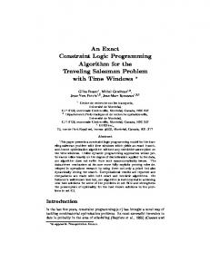
We’ve tested REVISE on several examples, including the important problem of representing diagnostic strategies in a modelbased reasoning system. Below are two examples. 4.1 Two Inverter Circuit In this example we present two extended diagnosis cases which illustrate the use of the preference graph to capture

1

diagnosis strategies. Consider the simple two inverter circuit in figure 1.

0 0 1

1 a

b

g1

2

c

g2

1 3 5

Figure 1: Two Inverter Circuit The normal and abnormal behaviour of the inverter gate is modelled by the rules below. We assume that our inverter gates have two known modes of erroneous comportment, either the output is always “0” (mode “stuck at 0”) or is always “1” (mode “stuck at 1”). The fault mode “unknown” describes unknown faults, with no predicted behaviour. The last argument, , is a time–stamp that permits the modelling of distinct observations in time. It is also implicit that an abnormality is permanent. 1 0

2

1

bottom 1 3 4

2 4

bottom 1 2

5

~s0_impossible 3 ~s1_impossible ~ab(_) ~fault_mode(_,_)

~s0_impossible ~s1_impossible ~single_fault_impossible ~ab(_) ~fault_mode(_,_)

4 ~s0_impossible ~single_fault_impossible ~ab(_) ~fault_mode(_,_)

0 1 0 1

0 1

1

0 1

2

~s0_impossible ~ab(_) ~fault_mode(_,_)

0 1

~single_fault_impossible ~ab(_) ~fault_mode(_,_)

bottom

The connections among components and nodes are described by:

~ab(_) ~fault_mode(_,_)

1 2

The first integrity rule below ensures that the fault modes are exclusive, i.e. to an abnormal gate at most one fault mode can be assigned. The second one enforces the assignment of at least one fault mode to anomalous components. The last integrity rule expresses the fact that to each node only one value can be predicted or observed at a given time. 1

2

1

2

0 1 1

2

1

2

Now we show how the preference graph can be used to implement distinct reasoning modes. The basic idea is to focus reasoning by concentrating on probable failures first (simple views, high abstraction level, etc ), to avoid reasoning in too large a detail. In this example, we’ll prefer single faults to multiple faults (i.e. more than one component is abnormal), fault mode “stuck at 0” to “stuck at 1” and the latter to the “unknown” fault mode. One possible combination of these two preferences is expressed using the following integrity rules and preference graph. This graph and its associated revisables are depicted in figure 2.

Figure 2: Reasoning Modes Preference Graph In the bottom level only and are revisables. Because neither of 0 , 1 and are revisables, the integrity rules enforce single “stuck at 0” faults. Level 1 and level 3 correspond to single “stuck at 1” faults and single “unknown faults.” Level 2 express possible multiple “stuck at 0” faults. Level 4 captures multiple “stuck at 0” or “stuck at 1” faults. Finally, all kind of faults, single or multiple, are dealt with in level 5. We could migrate the knowledge embedded in the last four previous integrity rules to the preference graph. This preference graph is more elaborate (but probably more intuitive) as shown in figure 3. The dashed boxes correspond to the levels of the previous preference graph and are labeled accordingly. This demonstrates how the meta–knowledge represented in the preference graph could move to the program, with a substancial reduction of the preference relation. If instead of 2 components we had 100, the extended graph we will have about 304 nodes and the smaller one is identical to the one of figure 2. The general conditions of the preference graph that allow this transference of information are the subject of further investigation.

ab(_) fm(_,_)

0

5

1 1 2

ab(_) fm(_,s0) fm(_,s1)

ab(g2) fm(g2,unk)

ab(g1) fm(g1,unk)

0 4

3

ab(g1) fm(g1,s1)

ab(g2) fm(g2,s1)

ab(_) fm(_,s0)

1

1 1 2

1 2

4.2 MULTIPLE MODELS AND HIERARCHY 2

ab(g1) fm(g1,s0)

1 2 0

ab(g2) fm(g2,s0)

In the rest of this section we will consider a small abstract device. We will focus on the use of different abstraction and diagnosis strategies and leave out the actual details of the models. This device is built from chips and wires and has a certain behaviour. If it does not show that behaviour, then we consider one of its parts abnormal.

bottom

% concept: structural hierarchy, % axiom: some part is defect, iff one its subparts is defect, % strategy: decompose the system into its subcomponents

bottom

Figure 3: Extended Preference Graph

Suppose that in the first experiment made the input is 0 and the values at nodes and are also 0 (see figure 4). These observations are modelled by the facts: 0 0

a

0

0 0

g1

b 0

g2

0 0

c

0

Figure 4: First Experiment

% first observation % contradiction found at highest level

In our case, either the chips can be faulty or the wires can be faulty. To check that, we use a functional model if available (in the case of the chips) or a physical model. As we will see later, our specified preference order leads us to suspect the chips first. % concept: functional/physical hierarchy. % a contradiction is found, if the functional model leads to % contradiction. If this is the case, check the physical models % of the suspected component (these axioms come later)

This program is contradictory with the following single preferred revision obtained at level 2: 1

2 2 0

1 0

The facts 0 1 1 1 0 1 describe the results of a second experiment made in the circuit. The above two experiments together generate, at level 5, the revisions below. Notice that the second one is at first sight non intuitive. We formulated the problem employing the consistency–based approach to diagnosis, therefore it is consistent with the observations to have both gates abnormal with “unknown” faults.

% no functional model for wires, % directly start with the physical model

When testing the chips, we use the functional hierarchy and get three function blocks fc1, fc2 and fc3. % enumeration of possible abnormal % components (functional decomposition) 1 3

2

The functions of these blocks and their interdependencies are described in an arbitrary way, below we show a very simple sequential relationship. % behaviour of single components in one model view % simple kind of sequential propagation, model valid % only if we just use chip model (no faulty wires) 1 2

1 2

1

3

3

2

% behaviour of components with fault mode 2 2

2

Now, we have two more observations, which tell us, that c1 is not functioning according to its fault mode 1 and c4 is not either. So, as we prefer fault mode 1 to fault mode 2 (as specified later in the preference ordering) the effect of the third observation is to focus on c4 in fault mode 1, while the effect of the fourth observation is to reconsider both c4 and c1 in fault mode 2. % third observation

3

1 1

We really find out, that the functional block fc1 malfunctions. Now we have to check, which physical components compose that functional block and which one of them is faulty. As functional block fc1 consists of two physical components c1 and c4, these two are our suspects after the first two observations.

% fourth observation

% second observation, restricts the found diagnoses to fc1

1 4

Finally, with a last observation, we restrict our suspect list again to c4 in fault mode 2. Finally, observation 6 leads us to consider unknown faults. % fifth observation

1

2 1

% concept: multiple models. % When a fault is found using the functional model, check the % physical chip models, prefer physical chip model 1 over % physical chip model 2.

% types

The functional decomposition need not be the same as the physical composition, functional component c1 consists of physical components c1 and c4), physical model 2 (ap2) corresponds to the unknown failure mode, we prefer physical mode 1, if it resolves the contradiction. 1 2 3

2 1 2 2 2 3

4

2 4

On the level of physical components we have descriptions of behavioural models, in our case models of the correct mode and two fault modes. We further have the assumption, that there is no other unknown fault mode. % behavioue single components in the physical model 1 1 2 3 4

1 2 3 4

2 2 2 2

1 2 3 4

% exclusive failure modes for chips in physical model 1 1

2 4

For the wires, we just have a physical model:

type(c1,chip)type(c2,chip) type(c3,chip)type(c4,chip)

1 2 3

% sixth observation

2

1 2 1 1 2

2

1 2

Finally, we specify a specific diagnosis strategy by using the preference order of revisables. The preference graph below starts to tes the most abstract hierarchy level ( ). If something is wrong, then go to the next hierarchy level (chips and wires) on this level, first consider chip faults with fault mode 1 first (level 1). Otherwise try single fault with fault mode 2 (level 2). If this doesn’t explain the behaviour try a double fault with fault mode 1 or a single unknown fault (3,4). Otherwise suspect faulty wires (level 5). If this does not work then everything is possible in the last level (6).

1 3 5

bottom 2 3 4

2 4 5

1 2 6

% behaviour of components with fault mode 1 1

1

The sequence of revisions and the revisable levels are listed below:

5 Level

REVISION ALGORITHM

Revisions The main motivation for this algorithm is that at distinct preference levels the set of revisables may differ, but it is necessary to reuse work as much as possible, or otherwise the preferred revisions algorithm will be prohibitively inefficient. We do so by presenting an extension to Reiter’s algorithm [Reiter, 1987], corrected in [Greiner et al., 1989], that fully complies with this goal. The preference revision process can be built upon this algorithm simply by calling it with the current set of revisables, as shown in section 3. This permits the reuse of the previous computations that matter to the current set of revisables. The algorithm handles arbitrary sets of assumptions, handles different sets of revisables at different levels, and provides a general caching mechanism for the computation of minimal “hitting sets” obtained at previous levels.

1 1 2 2 3 2 4 1 5 6 2

1

2

Table 1: Levels and Revisables Observation 1, Revisions at level 1: 1

4

1 4

1

1

1 1

2

2

1 2

3

3

1 3

Observation 2, Revisions at level 1: 1

4

1 4

1

1

1 1

Observation 3, Revisions at level 1: 1

4

1 4

Observation 4, Revisions at level 2: 1

4

2 4

1

1

2 1

Observation 5, Revisions at level 2: 1

4

2 4

Observation 6, Revisions at level 3: 1

2 1

1

2 4

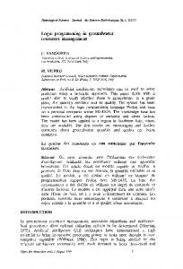
The main data structure is a DAG constructed from a set of conflict sets (all the inconsistencies) and a noncontradictory initial context which expresses what are the initial truth values of the revisables. An inconsistency is a support of contradiction. In our setting, these conflict sets are the intersection of a support set of with the set of revisables and their negations. Thus, a conflict set contains only literals that were already revised and literals that can be revised, which jointly lend support ot contradiction. Remark that the next algorithm is described independently of the initial context and of the type of revisable literals (they may be true positive literals that are allowed to become false through revision). A generalized–hitting–set directed–acyclic–graph (GHSDAG) is a DAG where nodes are labeled with sets of conflict sets. Edges are labeled with negations of revisables. In the basic algorithm (without pruning) the need for labeling nodes with sets of conflict sets is not evident. For clarity we’ll describe the basic algorithm assuming that there is only one conflict set in the label. After introducing pruning we’ll slightly revise the basic algorithm to cope with the more general case. In the following, new , is used to build the level specific GHS–DAG using the conflict sets stored in the GHS–DAG (used as the global cache). While computing the level specific DAG the global cache is updated accordingly. This latter GHS–DAG will be fed into the next iteration of algorithm 3.1 to minimize computation effort in less preferred levels. The minimal, level specific, revisions for a given set of revisables are obtained from new Conflict sets are returned by a theorem prover; as in [Reiter, 1987, Greiner et al., 1989] the algorithm tries to minimize the number of calls to the theorem prover. The set of all revisables is a non-contradictory set of literals Intuitively, if a literal (resp. ) belongs denoted by to then we allow to change its truth-value to false is a subset of A (resp. to true). A conflict set conflict set contains literals that cannot be simultaneously true (similar to the definition of NOGOOD [McDermott,

1991]). A context is a subset of The reader is urged to recourse to figure 5 when reading the basic algorithm below, where the initial context is and The set of inconsistencies, , contains the sets appearing in the figure. We assume, for simplicity, that the global GHS–DAG is empty and therefore in every step and new are equal. The nodes are numbered by order of creation. {~a,~b,~c} b

a

5

X

{a,b,~c} c

b {a,d}

a

b

{a,.~b}

9

c

{b,~a,~c} 3

{a,~b,~d} 2 d

1

$

10

6

{a,b,~c}

$

4

c

7

{b,c,~a}

c

a

$ 11

$

8

12

13

Figure 5: Basic Algorithm 0. Let be a set of conflict sets and context. The first time this algorithm is called GHS–DAG is empty. 1. Let be a set of revisables, a GHS-DAG and new an empty GHS-DAG. If is not empty then insert a clone of its root node in new Otherwise, insert in new an unlabeled node and a clone node in 2. Process the nodes in new in breadth–first order. Let be a node. The set contains the revisions of literals in the path from the root to the node and is the context at node To process node : (a) Define to be the set of edge labels on the path in new from the root down to node (empty if is the root). Let is not labeled then if for all then label and its clone with the special symbol Otherwise, label the node with one arbitrary such that Copy the label to its clone in If is already labeled denote its label by If then mark the node in new as closed. (c) If is labeled by a set , then for each , generate a new outgoing arc labeled by leading to a new node If an arc already exists in , from a clone of and label to some node , then copy the label of to in new Node becomes the clone of

Otherwise is created in

remains unlabeled and a clone arc

3. Return the resulting GHS–DAGs,

new

and

.

If the node is not labeled in step 2b then it was unexplored. The algorithm attempts to find a conflict set compatible with the current context. If there is no conflict then a revision is found (possibly not minimal) and it is marked with If a conflict set is found then it is intersected with the current revisables. If the intersection is empty a nonrevisable contradiction was found. Otherwise, the node must be expanded in order to restore consistency. This is accomplished by complementing a single revisable literal in the conflict set. This process is iterated till there are no more nodes to expand. An access to the set of inconsistencies in step 2b can be regarded has a request to the theorem prover to compute another conflict set. Also, notice in the end new will be contained in All the revisions wrt the specified set of revisables can be obtained from new We now define pruning enhancements to new such that, in the end, the minimal revisions can be obtained from this new DAG. The result of the application of the next optimizations to the problem described in figure 5 is shown in figure 6. Node 5 is obtained by application of pruning step 3a. Node 6 is reused by node 3 and nodes 7 and 8 were closed by node 4. {~a,~b,~c} b

a {a,~b}

1

{b,~a,~c}

5

a

b {a,b,~c}

6

c $

3

4

c X

7

c X

8

(b) If

Figure 6: Pruning Enhancements 1. Reusing nodes: this algorithm will not always generate a new node as a descendant of node in step 2c: (a) If there is a node in new such that , then let the –arc under point to this existing node and reflect this in its clone Thus, these nodes will have more than one in parent. as described in the basic (b) Otherwise generate algorithm.

2. Closing: If there is a node in new labeled with and , then close node and its clone in

set condition); second it directs the search to the sub-DAG with less nodes remaining to be explored, reusing maximally work done before.

3. Pruning: Let be the label of node in step 2b, and be another node in new labeled with conflict set Attempt to prune new and as follows:

It can be shown that if the number of conflict sets is finite, and they themselves are finite, then this algorithm computes the minimal revisions and stops. It is known this problem is NP-Hard: an exponential number of minimal revisions can be generated. Under the previous conditions algorithm 3.1 is sound and complete, if it has a finite number of preference rules (wrt def. 3.1).

(a) Pruning

and then relabel with . For in the –arc under is any no longer allowed. The node connected by this arc and all of its descendants are removed, except for those nodes with another ancestor which is not being removed. This step may eliminate the node currently being processed. (b) Pruning : Let and be the clones of and in , respectively. i. If and for some in Apply the procedure in 3a) to taking into account that more than one set may label the node: remove all the that verify the condition, insert in the label and retain –edges and descendant nodes such that belongs to some of the remaining sets. Notice this procedure was already applied to new

: If

The computation of the preferred revisions of example in section 4.1 is portrayed in figure 7, with the obvious abreviations for the literals appearing. The whole example has 25 minimal inconsistencies, i.e. minimal support sets of The computations done at each level are bounded by the labeled bold lines. The dashed line represents the bound of the level specific GHS–DAG at levels , 2 and 4. These leves all nodes are closed, i.e. there are no revisions. Notice that pruning steps 3a) and 3(b)ii were applied between the node initially labeled with 2 and the nodes labeled with 1 0 and 1 1 . {~ab(g1)} ab(g1)

new

ii. If the condition in 3a) was verified by then insert in the label of the set

and

The reuse and closing of nodes avoids redundant computations of conflict sets. The closing rule also ensures that in the end the nodes labeled with are the minimal revisions. The pruning strategy is based on subset tests, as in Reiter’s original algorithm, but extended to take into account the contexts and revisables. The principle is simply that given two conflict sets one contained in the other, the bigger one can be discarded when computing minimal revisions. The algorithm handles the case when a conflict set is a subset of another wrt the revisables, but not if the revisables are not considered. Also notice that condition 3(b)ii is redundant if step 3(b)i was applied. The need to consider nodes labeled by several conflict sets is justified by the pruning step 3(b)ii: the set is minimal wrt the current set of revisables. We store this set in the global cache for later use by the algorithm. To reap the most benefit from this improvement it is necessary to change step 2b) by introducing the following test:

{ab(g1),~fm(g1,s0),~fm(g1,s1),~fm(g1,uk)} fm(g1,s0)

{ab(g1),fm(g1,s0)} X bottom, 2, 4

fm(g1,uk)

fm(g1,s1)

{~ab(g2)} {fm(g1,uk),~s0i} {fm(g1,uk),~s1i}

{ab(g1),fm(g1,s1)} X

ab(g2)

{ab(g2),~fm(g2,s0),~fm(g2,s1),~fm(g2,uk)} fm(g2,uk)

bottom, 2

{fm(g1,uk), fm(g2,uk),~sfi}

fm(g2,s0)

fm(g2,s1)

{fm(g1,uk),~s0i}

{ab(g2),fm(g2,s1)} X

s0i

{fm(g1,uk),fm(g2,s0),~sfi}

1,3 sfi

sfi

{fm(g1,uk),~s1i}

4

s1i

“If is labeled by conflict sets, i.e. it was previously computed, then intersect these sets with Select from the obtained sets a minimal one such that the number of nodes below this node, wrt , is maximum. Relabel with this set.” The heuristic in the modified step is to use a minimal set wrt to the current set of revisables having the most of search space explored. This has two main advantages: first, the new algorithm can ignore redundant branches (the minimal

5

$

$

Figure 7: Preferred Revisions Computation As the reader may notice, the higher the level is in the preference graph the deeper is the GHS–DAG generated. This corresponds to what is desired: preferred revisons should be obtained with less theorem proving costs.

The efficiency of the algorithm is highly dependent on the order in which conflict sets are generated. It is possible to 1 conflict sets with a devise very nasty examples having single revision of cardinality 1, where the above algorithm has to explore and generate an exponential GHS–DAG. One possible solution to this problem is to guarantee that the theorem prover only returns minimal sets of inconsistencies. This can be done by an intelligent search strategy used by the theorem prover. This topic will be the subject of a future paper.

6

COMPARISONS AND CONCLUSIONS

We start by concentrating on diagnosis strategies, only recently approached in [Struss, 1989, Dressler and Bottcher, 1992, Bo¨ ttcher and Dressler, 1994], where they discuss the necessity of including diagnostic strategies in a modelbased reasoning system such as when to use structural refinement, behavioural refinement, how to switch to different models, and when to use which simplifying assumptions. [Dressler and Bottcher, 1992] also gives an encoding of these preferences on top of an NM-ATMS, using both default rules of the form discussed earlier for local preferences and metalevel rules for explicitly specifying global preference during the revision process. The disadvantage of the implementation discussed in [Dressler and Bottcher, 1992] and its extended version is that the specification of these preferences is too closely intertwined with their implementation (NM-ATMS plus belief revision system on top) and that different preferences must be specified with distinct formalisms. Default logic allows a rather declarative preferences specification, while the metarules of [Dressler and Bottcher, 1992] for specifying global preferences have a too procedural flavour. In contrast, REVISE builds upon a standard logic programming framework extended with the explicit specification of an arbitrary (customizable) preference relation (including standard properties ([Kraus et al., 1990, Nejdl, 1991b]) as needed). Expression of preferences is as declarative as expressing diagnosis models, uses basically the same, formalism and is quite easy to employ according to our experience. In our diagnosis applications, although our implementation still has some efficiency problems due to being implemented as a meta-interpreter in Prolog (a problem which can be solved without big conceptual difficulties), we are very satisfied with the expressiveness of REVISE and how easy it is to express in it a range of important diagnosis strategies. We are currently investigating how to extend our formalism for using an order on sets of diagnoses/sets of worlds/sets of sets of assumption sets, instead of the current order on diagnoses/worlds (or assumption sets). Without this greater expressive power we are not able to spell out strategies depending on some property out of the whole set of diagnoses (two or three of such strategies are discussed in a belief revision framework in [B¨ottcher and Dressler, 1994]).

Revising a knowledge base has been the main topic for belief revision systems and it is quite interesting to compare REVISE to a system like IMMORTAL [Chou and Winslett, 1991]. IMMORTAL starts from a consistent knowledge base (not required by our algorithm) and then allows updating it. These updates can lead to inconsistencies and therefore to revisions of the knowledge base. In contrast to our approach, all inconsistencies are computed statically before any update is done, which for larger examples is not feasible, in our opinion. Also, due to their depth-first construction of hitting sets, they generate non-minimal ones, which have to be thrown away later. (This could be changed by employing a breadth-first strategy.) Priority levels in IMMORTAL are a special kind of our preference levels, where all levels contain disjoint literals and the levels are modular, both of which properties can be relaxed in REVISE (and have to be in some of our examples). Accordingly, IMMORTAL does not need anything like our DAG global data structure for caching results between levels. Additionally, IMMORTAL computes all conflict sets and then removes non-updateable literals, in general leading to duplicates; therefore, in our approach, we have less conflict sets and so a faster hitting sets procedure (and less theorem prover costs). Comparing our work to database updates and inconsistency repairing in knowledge bases, we note that most of this work takes some kind of implicit or explicit abductive approach to database updates, and inconsistency repairs are often handled as a special case of database update from the violated contraints (such as in [W¨uthrich, 1993]). If more than one constraint is violated this leads to a depth-first approach to revising inconsistencies which does not guarantee minimal changes. Moreover, we do not know of any other work using general preference levels. All work which uses some kind of priority levels at all uses disjoint priority levels similar to the IMMORTAL system. Compared to other approaches, which are based on specific systems and specific extensions of these systems such as [Dressler and Bottcher, 1992], REVISE has big advantages in the declarativity, and is built upon on a sound formal logic framework. We therefore believe the REVISE system is an appropriate tool for coding a large range of problems involving revision of knowledge bases and preference relations over them. REVISE is based on sound logic programming semantics, described in this paper, and includes some interesting implementation concepts exploiting relationships between belief revision and diagnosis already discussed in very preliminary form in [Nejdl, 1991a]. While REVISE is still a prototype, we are currently working on further improving its efficiency, and are confident the basic implementation structure of the current system provides an easily extensible backbone for efficient declarative knowledge base revision systems.

Acknowledgements We thank project ESPRIT Compulog 2, JNICT Portugal and the Portugal/Germany INIDA program for their support. References [Alferes, 1993] Jos´e Ju´ lio Alferes. Semantics of Logic Programs with Explicit Negation. PhD thesis, Universidade Nova de Lisboa, October 1993. [B¨ottcher and Dressler, 1994] Claudia B¨ottcher and Oskar Dressler. Diagnosis process dynamics: Putting diagnosis on the right track. Annals of Mathematics and Artificial Intelligence, 11(1–4), 1994. Special Issue on Principles of Model-Based Diagnosis. To appear. [Chou and Winslett, 1991] Timothy S-C Chou and Marianne Winslett. Immortal: A model-based belief revision system. In In Proc. KR’91, pages 99–110, Cambridge, April 1991. Morgan Kaufmann Publishers, Inc. [de Kleer, 1991] Johan de Kleer. Focusing on probable diagnoses. In Proceedings of the National Conference on Artificial Intelligence (AAAI), pages 842–848, Anaheim, July 1991. Morgan Kaufmann Publishers, Inc. [Dressler and Bottcher, 1992] O. Dressler and C. Bottcher. Diagnosis process dynamics: Putting diagnosis on the right track. In Proc. 3nd Int. Workshop on Principles of Diagnosis, 1992. [Friedrich and Nejdl, 1992] Gerhard Friedrich and Wolfgang Nejdl. Choosing observations and actions in modelbased diagnosis-repair systems. In In Proc. KR’92, pages 489–498, Cambridge, MA, October 1992. Morgan Kaufmann Publishers, Inc. [Gelder et al., 1991] A. Van Gelder, K. A. Ross, and J. S. Schlipf. The well-founded semantics for general logic programs. Journal of the ACM, 38(3):620–650, 1991. [Greiner et al., 1989] Russell Greiner, Barbara A. Smith, and Ralph W. Wilkerson. A correction to the algorithm in Reiter’s theory of diagnosis. Artificial Intelligence, 41(1):79–88, 1989. [Hamscher et al., 1992] W. Hamscher, L. Console, and J. de Kleer. Readings in Model-Based Diagnosis. Morgan Kaufmann, 1992. [Kakas and Mancarella, 1991 ] A.C. Kakas and P. Mancarella. Generalized stable models: A semantics for abduction. In Proc. ECAI’90, pages 385–391, 1991. [Kraus et al., 1990] Sarit Kraus, Daniel Lehmann, and Menachem Magidor. Nonmonotonic reasoning, preferential models and cumulative logics. Artificial Intelligence, 44(1–2):167–207, 1990. [Lackinger and Nejdl, 1993 ] Franz Lackinger and Wolfgang Nejdl. DIAMON: A model-based troubleshooter based on qualitative reasoning. IEEE Expert, February 1993. [McDermott, 1991] Drew McDermott. A general framework for reason maintenance. Artificial Intelligence, 50(3):289–329, 1991.

[Nejdl and Banagl, 1992 ] Wolfgang Nejdl and Markus Banagl. Asking about possibilities — revision and update semantics for subjunctive queries. In In Proc. KR’92, Cambridge, MA, October 1992. Also appears in the ECAI-Workshop on Theoretical Foundations of Knowledge Representation and Reasoning, August 1992, Vienna. [Nejdl, 1991a] Wolfgang Nejdl. Belief revision, diagnosis and repair. In Proceedings of the International GI Conference on Knowledge Based Systems, M u¨ nchen, October 1991. Springer-Verlag. [Nejdl, 1991b] Wolfgang Nejdl. The P-Systems: A systematic classification of logics of nonmonotonicity. In Proceedings of the National Conference on Artificial Intelligence (AAAI), pages 366–372, Anaheim, CA, July 1991. [Pereira and Alferes, 1992] L. M. Pereira and J. J. Alferes. Well founded semantics for logic programs with explicit negation. In B. Neumann, editor, European Conference on Artificial Intelligence, pages 102–106. John Wiley & Sons, Ltd, 1992. [Pereira et al., 1993a] L. M. Pereira, J. N. Apar´ıcio, and J. J. Alferes. Non–monotonic reasoning with logic programming. Journal of Logic Programming. Special issue on Nonmonotonic reasoning, pages 227–263, 1993. [Pereira et al., 1993b] L. M. Pereira, C. Dam´asio, and J. J. Alferes. Diagnosis and debugging as contradiction removal. In L. M. Pereira and A. Nerode, editors, 2nd Int. Ws. on Logic Programming and NonMonotonic Reasoning, pages 316–330. MIT Press, 1993. [Pereira et al., 1993c] L. M. Pereira, C. V. Dam´asio, and J. J. Alferes. Debugging by diagnosing assumptions. In Automatic Algorithmic Debugging, AADEBUG’93. Springer–Verlag, 1993. [Pereira et al., 1993d] L. M. Pereira, C. V. Dam´asio, and J. J. Alferes. Diagnosis and debugging as contradiction removal in logic programs. In Proc. 6th Portuguese Conference On Artificial Intelligence (EPIA’93). Springer– Verlag, LNAI 727, 1993. [Przymusinska and Przymusinski, 1990 ] H. Przymusinska and T. Przymusinski. Semantic issues in deductive databases and logic programs. In R. Banerji, editor, Formal Techniques in AI, a Sourcebook, pages 321–367. North Holland, 1990. [Reiter, 1987] R. Reiter. A theory of diagnosis from first principles. AI, 32:57–96, 1987. [Struss, 1989] P. Struss. Diagnosis as a process. In Working Notes of First Int. Workshop on Model-based Diagnosis, Paris, 1989. Also in [Hamscher et al., 1992]. [W¨uthrich, 1993] B. W¨uthrich. On updates and inconsistency repairing in knowledge bases. In Proceedings of the International IEEE Conference on Data Engineering, Vienna, Austria, April 1993.