on the natural interval extension of constraints and captures both the orig- inal definition ... of each variable in a constraint: domain narrowing for variables occurring ..... Newton method when a cheaper method (straight evaluation) is available.
Appears in: Procs. of the 16th Intl. Conf. on Logic Programming, p. 230–244, The MIT Press, 1999
Revising hull and box consistency Fr´ ed´ eric Benhamou, Fr´ ed´ eric Goualard, Laurent Granvilliers IRIN, Universit´e de Nantes B.P. 92208, F-44322 Nantes Cedex 3 Jean-Fran¸ cois Puget ILOG S.A. B.P. 85, F-94253 Gentilly Cedex
Abstract Most interval-based solvers in the constraint logic programming framework are based on either hull consistency or box consistency (or a variation of these ones) to narrow domains of variables involved in continuous constraint systems. This paper first presents HC4, an algorithm to enforce hull consistency without decomposing complex constraints into primitives. Next, an extended definition for box consistency is given and the resulting consistency is shown to subsume hull consistency. Finally, BC4, a new algorithm to efficiently enforce box consistency is described, that replaces BC3—the “original” solely Newton-based algorithm to achieve box consistency—by an algorithm based on HC4 and BC3 taking care of the number of occurrences of each variable in a constraint. BC4 is then shown to significantly outperform both HC3 (the original algorithm enforcing hull consistency by decomposing constraints) and BC3.
1
Introduction
Finite representation of numbers precludes computers from exactly solving continuous problems. Interval constraint solvers such as Prolog IV, Numerica [14], and ILOG Solver [12], tackle this problem by relying on interval arithmetic [10] to compute verified approximations of the solutions to constraint systems. Domains are associated to every variable occurring in the problem, and solving a particular constraint then lies in eliminating some of the values of these domains for which the constraint does not hold (inconsistency), using local consistency techniques and filtering [9]. In practice, enforced consistencies only approximate perfect local consistency since some solutions may be unrepresentable with floating-point numbers. Two worth mentioning approximate consistencies are hull consistency [1] and box consistency [2]. Most interval constraint solvers are based on either one of them. Enforcing hull consistency usually requires decomposing the user’s constraints into so-called primitive constraints [4].
A well known drawback of this method is that the introduction of new variables induced by the decomposition hinders efficient domain tightening. On the other hand, the original algorithm enforcing box consistency processes constraints without decomposing them but is not at best with constraints involving many variables with few occurrences. In [6], some of the authors have presented DecLIC, a CLP language allowing the programmer to choose the “best fitted” consistency to use for each constraint of a system; however, deferring the choice of the consistency to the user spoils the declarativity of the language. In this paper, HC4, an algorithm to enforce hull consistency is first presented, that traverses repeatedly from top to bottom and conversely the tree-structured representation of constraints; consequently, decomposition of complex constraints into “primitives” is no longer needed. Next, a slightly extended definition of box consistency is given, that no longer solely relies on the natural interval extension of constraints and captures both the original definition of box consistency [2] and the one by Collavizza et al. [5]. A new algorithm (BC4) permitting to efficiently enforce box consistency is then given. BC4 adapts the computation method to the number of occurrences of each variable in a constraint: domain narrowing for variables occurring only once in a constraint (which is one of the weaknesses of the “original” Newton-based method to enforce box consistency) is obtained by using HC4; variables occurring more than once are handled by searching “extreme quasi-zeros” using an interval Newton method as described in the original paper [2]. The rest of this paper is organized as follows: Section 2 presents the basics related to interval constraint solving. Section 3 presents hull consistency along with the usual scheme used to enforce it [4]; next, Algorithm HC4 to enforce hull consistency without decomposing constraints is described and its properties are pointed out. Section 4 first presents the extended definition for box consistency; Algorithm BC4 to efficiently enforce box consistency is then given. Section 5 comments results obtained on a prototype implementing BC4. Last, Section 6 summarizes the paper’s contribution and points out some directions for future research.
2
Preliminary notions
In order to model the change from continuous domains to discrete domains induced by the shift from reals to machine numbers, Benhamou and Older [3] have introduced the notion of approximate domain over the set of reals1 R: an approximate domain A over R is a subset of the power set of R, P(R), closed under intersection, containing R, and for which the inclusion is a well-founded ordering. The approximation w.r.t. A of a real relation ρ, 1 The original definition is more general but the one given here is sufficient for our purpose.
written apxA (ρ), is then defined as the intersection of all the elements of A containing ρ. This section focuses on two widely used approximation sets over R, namely intervals and unions of intervals. The shift from reals to intervals is first described; interval constraints are then introduced; finally, the basics related to interval constraint solving are presented. Let R be the set of reals compactified with the infinities {−∞, +∞} in the obvious way, and F ⊂ R a finite subset of reals corresponding to binary floating-point numbers in a given format [8]. Let F∞ be F ∪ {−∞, +∞}. For every g ∈ F∞ , let g+ be the smallest element in F∞ greater than g, and g− the greatest element in F∞ smaller than g (with the conventions: (+∞)+ = +∞, (−∞)− = −∞, (+∞)− = max(F), (−∞)+ = min(F)). A closed/open floating-point interval is a connected set of reals whose lowest upper bound and greatest lower bound are floating-point numbers. The following notations are used as shorthands: [g..h] ≡ {r ∈ R | g 6 r 6 h}, [g .. h) ≡ {r ∈ R | g 6 r < h}, etc. Let I◦ be the set of closed/open floatingpoint intervals and I� the set of closed floating-point intervals. Let U◦ be the set of unions of disjoint closed/open intervals, and U� the restriction of U◦ to unions of disjoint closed intervals. Let I (resp. U) denote the set of intervals (resp. unions of intervals) when the distinction between closed and closed/open bounds is useless. For the sake of clarity and otherwise explicitly stated, we will only consider hereafter (unions of) closed floatingpoint intervals. A Cartesian product of n intervals B = I1 × · · · × In is called a box ; a domain D is either an interval I or a union U of disjoint intervals. A non-empty interval I = [g .. h] is said to be canonical whenever h 6 g+ . An n-ary box B is canonical whenever intervals I1 , . . . , In are canonical. In the sequel, a real (resp. interval) constraint is an atomic formula built from a real (resp. interval)-based structure and a set of real (resp. interval)valued variables. Given a real constraint c, let ρc denote the underlying relation, Var(c) be the set of variables occurring in c, and Multiplicity(v, c) the multiplicity (i.e. the number of occurrences) of the variable v in the constraint c. An interval extension of f : Rn → R is a mapping F : In → I such that for all I1 , . . . , In ∈ I : r1 ∈ I1 , . . . , rn ∈ In ⇒ f (r1 , . . . , rn ) ∈ F (I1 , . . . , In ). An interval extension of a relation ρ ⊆ Rn is a relation R ⊆ In such that for all I1 , . . . , In ∈ I : ∃r1 ∈ I1 . . . ∃rn ∈ In s.t. (r1 , . . . , rn ) ∈ ρ ⇒ (I1 , . . . , In ) ∈ R. A real relation ρ may be conservatively approximated by the smallest (w.r.t. set inclusion) union of disjoint boxes Union(ρ) = apxU (ρ) (resp. the smallest box Hull(ρ) = apxI (ρ)) containing it. In the sequel, the following approximations are used: Union◦ (ρ) = apxU◦ (ρ), Union� (ρ) = apxU� (ρ), Hull◦ (ρ) = apxI◦ (ρ), and Hull� (ρ) = apxI� (ρ). An n-ary interval operation � is called the natural interval extension of an n-ary real operation ♦ if for all I1 , . . . , In ∈ I : �(I1 , . . . , In ) = Hull({♦(x1 , . . . , xn ) | x1 ∈ I1 , . . . , xn ∈ In }). The natural interval extension of a function f : Rn → R is the interval function obtained from f by replacing each con-
stant r by Hull({r}), each variable by an interval variable, and each operation by its natural interval extension. Given an n-ary real constraint c, let πk (ρc ) = {rk ∈ R | ∃r1 , . . . , ∃rn ∈ R s.t. (r1 , . . . , rn ) ∈ ρc } be the k-th projection of ρc . Given a real constraint c(x1 , . . . , xn ), a constraint solver aims at reducing the domains associated to variables x1 , . . . , xn . This reduction process is abstracted by the notion of constraint narrowing operators [1] (shortened thereafter to CNOs) which are complete, contracting, and monotone functions taking as input a box and returning a box from which have been discarded some of the elements which do not belong to ρc . Due to space requirements, we only give proof sketches for the properties stated hereinafter.
3
Hull consistency and related algorithms
Discarding all values of a box B for which a real constraint c does not hold is not achievable in general. Section 3.1 presents a coarser consistency called hull consistency [3] consisting in computing the smallest box that contains ρc ∩ B. Section 3.2 describes HC4, a new algorithm tackling one of the drawbacks of the original algorithm used to enforce hull consistency, that is, the decomposition of the user’s constraints.
3.1
Hull consistency: the original scheme
The original definition of hull consistency is based on the approximate domain I� , though it might easily be defined on I◦ : Definition 3.1 (hull consistency [3]). A real constraint c is said hull consistent w.r.t. a box B if and only if B = Hull� (ρc ∩ B). Due to round-off errors introduced by the use of floating-point numbers, computing the interval enclosure of a real set S is a difficult task in itself. Moreover, the precision of many arithmetic functions such as exp, cos. . . is not guaranteed by the IEEE 754 standard [8]; consequently, their actual precision is implementation dependent. Algorithm HC32 [2, 4] partly overcomes this problem by enforcing hull consistency over a decomposition c of simple—primitive—constraints rather than considering the user constraint c. For example, the constraint c : x + y ∗ z = t might be decomposed into c = {y ∗ z = α, x + α = t} with the addition of the new variable α. Formally, given a real n-ary constraint c and a box B, let ρc (k) (B) be dec
dec
2
HC3 is our own denomination for Algorithm Nar given in [2] and is justified by its very close relation to AC3.
the k-th canonical extension of ρc w.r.t. B defined as follows [13]: ρc (k) (B) = {rk ∈ R | ∃r1 ∈ I1 , . . . , ∃rk−1 ∈ Ik−1 , ∃rk+1 ∈ Ik+1 , . . . , ∃rn ∈ In
s.t.
(r1 , . . . , rn ) ∈ ρc }
A constraint c is called a primitive constraint on the approximate domain A if and only if one can exhibit n projection narrowing operators Nc1 , . . . , Ncn , defined from An to A, such that: ∀D = D1 × · · · × Dn , ∀k ∈ {1, . . . , n} : Nck (D) = apxA (ρc (k) (D) ∩ Dk ). The CNOs for primitive constraints are implemented using relational interval arithmetic [4] (see an example below). The main advantage of such an approach is that computation of hull consistency can be implemented very efficiently for the set of simple constraints supported by the constraint programming system. The drawbacks are that the introduction of new variables due to the decomposition process drastically hinders domain tightening for the variables the user is interested in. As pointed out in [2], this is particularly true when the same variables appear more than once in the constraints since each occurrence of a variable v is considered as a new variable v ′ with the same domain as v (dependency problem [10]). Example 3.1 (A CNO for c : x + y = z). Enforcing hull consistency for the constraint c : x + y = z and domains Ix , Iy , and Iz , is done by computing the common fixed-point included in B = Ix × Iy × Iz of the following projection operators: Nc1 (B) = Ix ∩ (Iz ⊖ Iy ), Nc2 (B) = Iy ∩ (Iz ⊖ Ix ), and Nc3 (B) = Iz ∩ (Ix ⊕ Iy ), where ⊖ and ⊕ are interval extensions of − and + defined as: [a .. b] ⊕ [c .. d] = [a + c .. b + d], and [a .. b] ⊖ [c .. d] = [a − d .. b − c]. As pointed out by Van Emden [13], the projection operators Nc1 ,Nc2 ,Nc3 , for a constraint of the form x ♦ y = z may all exist even if the function ♦ has no inverse. For example, consider the case where ♦ stands for the multiplication over I� : Nc1 computes the smallest union of intervals containing the set {rx ∈ Ix | ∃ry ∈ Iy , ∃rz ∈ Iz : rx × ry = rz }. Hence, it is defined even when 0 ∈ Iy .
3.2
HC4: a new algorithm for hull consistency
Algorithm 1 presents the HC4 algorithm which takes as input a set of constraints and a box, and narrows the variables’ domains as much as possible. Algorithm HC4 is very similar to Algorithm HC3 [1] except that input constraints c1 , . . . , cm , are user’s constraints instead of decomposed constraints, and that constraint narrowing operators associated to the constraints are implemented by Algorithm HC4revise, whose description follows. Algorithm HC4 shares the following properties with HC3: if the computation of HC4revise terminates for any constraint and any box, HC4 terminates; the algorithm is complete: the output Cartesian product of domains is a superset of the declarative semantics of the constraint system included
in the input box; the algorithm is confluent: the output is independent of the reinvocation order of constraints. Algorithm 1: HC4 algorithm
HC4(in {c1 , . . . , cm } ; inout B = I1 × · · · × In ) begin S ← {c1 , . . . , cm } while (S = 6 ∅ and B 6= ∅) do c ← choose one ci in S B ′ ← HC4Revise(c,B,I� ) if (B ′ 6= B) then S ← S ∪ {cj | ∃xk ∈ Var(cj ) ∧ Ik′ 6= Ik } B ← B′ else % HC4revise not idempotent: next call on c may further narrow domains S ← S \ {c} endif endwhile end
These properties are proved in the same way as for HC3 (see [11]) once HC4revise has been proved to be a constraint narrowing operator (Prop. 1). HC4 improves the compilation time (generation of primitives is useless), the solving time (no propagation needed between different primitive constraints for a given user’s constraint), and the memory size. Algorithm 2: HC4revise algorithm
HC4revise( in c = r(t1 , . . . , tp ): real constraint; inout B: box; in A: approximate domain) begin DA ← B foreach i ∈ {1, . . . , p} do ForwardEvaluation(ti ,DA ) endforeach BackwardPropagation(c,DA ) B← Hull� (DA ) end
Algorithm 2 presents HC4revise, the new algorithm implementing the constraint narrowing operators used in HC4. Once more, note that HC4revise considers the user’s constraints rather than primitives generated by decomposition: A real constraint r(t1 , . . . , tp ) is represented by an attribute tree where the root node contains the p-ary relation symbol r, and terms ti are composed of nodes containing either a variable, a constant, or an operation symbol. Moreover, each node but the root contains two interval attributes
t.fwd (synthesized) and t.bwd (inherited). Given a real constraint and a box B, Algorithm HC4revise proceeds in two consecutive stages: Algorithm 3: Forward evaluation algorithm
ForwardEvaluation( inout t: attribute tree; in DA = D1 × · · · × Dn : Cartesian product of domains) begin case (t) of % a term ♦(t1 , . . . , tj ): foreach i ∈ {1, . . . , j} do ForwardEvaluation(ti ,DA ) endforeach t.fwd ← �(t1 .fwd , . . . , tj .fwd ) % a constant a: t.fwd ← apxA ({a}) xk : % a variable t.fwd ← Dk endcase end
1. The forward evaluation phase (see Alg. 3 and Fig. 1) is a traversal of the terms from leaves to roots in order to evaluate in t.fwd the natural interval extension of every sub-term t of the constraint; 2. The backward propagation phase (see Alg. 4 and Fig.2) is a traversal of the tree-structured representation of the constraint from root to leaves in order to evaluate in every t.bwd a projection narrowing operator associated to the father of node t. More precisely, two kinds of node are considered: – given the root node r(t1 , . . . , tp ), attributes tk .bwd (k ∈ {1, . . . , p}) are computed by the k-th projection narrowing operator of the constraint r(x1 , . . . , xp ), where x1 ∈ t1 .fwd , . . . , xp ∈ tp .fwd ; – given a term th+1 ≡ ♦(t1 , . . . , th ), attributes tk .bwd (k ∈ {1, . . . , h}) are computed by the k-th projection narrowing operator of the constraint xh+1 = ♦(x1 , . . . , xh ), where xi ∈ ti .fwd for all i ∈ {1, . . . , h}, and xh+1 ∈ th+1 .bwd ; intuitively, variables xi simulate the new ones introduced by the decomposition process. During the backward propagation phase, the algorithm may be prematurely ended by the computation of an empty interval in some t.bwd . The constraint is then inconsistent w.r.t. the initial domains. If the computation is successful, the domain of each variable xi in the constraint is intersected with the one in xi .bwd .
Note: Backward propagation in a term is quite similar to automatic differentiation in reverse mode [7] for computing the partial derivatives of a real function: after the forward evaluation, the aim is either to evaluate the projection narrowing operators, or the partial derivatives for each node containing an operation symbol. At the end of the traversal in the tree, the domains are either intersected, or the derivatives summed. Algorithm 4: Backward propagation algorithm
BackwardPropagation(inout t: attribute tree; inout DA = D1 × · · · × Dn : Cartesian product of domains) begin case (t) of r(t1 , . . . , tm ): �% The root node c ← r(x1 , . . . , xm ) ′ DA ← (t1 .fwd , . . . , tm .fwd ) foreach i ∈ {1, . . . , m} do ′ ti .bwd ← πi (apxA (ρc ∩ DA )) BackwardPropagation(ti ,DA ) endforeach % A term ♦(t1 , . . . , th ): � below the root c ← ♦(x1 , . . . , xh ) = xh+1 ′ DA ← (t1 .fwd , . . . , th .fwd , t.bwd ) foreach i ∈ {1, . . . , h} do ′ ti .bwd ← πi (apxA (ρc ∩ DA )) BackwardPropagation(ti ,DA ) endforeach % A variable xj : Dj ← Dj ∩ t.bwd % Domains intersected to take into % account multiple occurrences of xj endcase end
Example 3.2. Figures 1 and 2 illustrate the computation of HC4revise over the constraint 2x = z − y 2 , with domains Ix = [0 .. 20], Iy = [−10 .. 10], and Iz = [0 .. 16]. Backward propagation at the root node computes [0 .. 40] ∩ [−100 .. 16] (the intersection corresponds to the interpretation of the equality between intervals) in (×(2, x)).bwd and (−(z,ˆ(y, 2))).bwd . Backward propagation at the root node of term ×(2, x) computes in x.bwd the interval I included in [0 .. 20] (result of forward evaluation) which verifies 2 × Ix = [0 .. 16]. Finally, the new domains (located in the grey nodes) are Ix = [0 .. 8], Iy = [−4 .. 4], and Iz = [0 .. 16]. Proposition 1. Given an n-ary real constraint c, Algorithm HC4revise implements a constraint narrowing operator for c. Proof. Follows from the fact that HC4revise consists essentially in applying
some primitive CNOs at each node of a finite tree, and that a composition of CNOs is also a CNO. Let HC4revise⋆ be Algorithm HC4revise where, given a node t, the attribute t.bwd is not eventually intersected with t.fwd .
= [0 .. 16]
2
×
[0 .. 40 ]
[0 .. 8]
[2 .. 2 ]
x
[0 .. 16]
[0 .. 20 ]
[0 .. 16]
z
−
[−100 .. 16 ]
[0 .. 16]
[0 .. 16 ]
y
[−4 .. 4]
ˆ
[0 .. 100 ]
2
[−10 .. 10 ]
2
Figure 1: Annotated tree for the forward evaluation in the constraint 2x = z − y 2
= [0 .. 16]
2
×
[2 .. 2 ]
[0 .. 16]
[0 .. 40 ]
[0 .. 8]
x
[0 .. 20 ]
[0 .. 16]
z
−
[0 .. 16 ]
[−4 .. 4]
[−100 .. 16 ]
[0 .. 16]
y
ˆ
[0 .. 100 ]
2
[−10 .. 10 ]
2
Figure 2: Annotated tree for the backward propagation in the constraint 2x = z − y 2
As stated by the following proposition, invoking Algorithm HC4 on a set of constraints C and a box B is equivalent to the invocation of Algorithm HC3 on B and the set of constraints generated by the decomposition of the constraints in C into primitives: Proposition 2. Given C a set of real constraints and B a box, [ the output box of HC4(C,B) is equal to the one of HC3(C ,B), where C = c . dec
dec
dec
c∈C
Proof. The proof is done by noticing that HC4 and HC3 use the same narrowing operators, and that the node attributes in HC4revise mimic the new variables in HC3. The proof then follows since the application order of the same constraint narrowing operators does not influence the fixed-point (confluency property of propagation algorithms [11]).
4
Box consistency and related algorithms
Box consistency [2] has been introduced to avoid decomposing constraints, thus tackling the dependency problem for variables with many occurrences. Section 4.1 generalizes its definition and surveys the original method used to enforce it. Some connections between Algorithm HC4revise and box consistency are then stated. Finally, Section 4.2 presents a new algorithm to enforce box consistency that avoids relying on the computationally expensive Newton method when a cheaper method (straight evaluation) is available.
4.1
Box consistency
The original box consistency definition [2] is based on I� and on the natural interval extension of constraints. It is generalized below by permitting the use of other interval extensions, and by parameterizing it with two approximate domains. This last modification allows us to take into account some variations over the original definition such as the one given by Collavizza et al. [5], where quasi-zeros are approximated by open intervals while the output result is a closed one. The definition applies to (possible) different interval extensions of the original real constraint to define the projections. Definition 4.1 (BoxA1 ,A2 ,Γ consistency). Given A1 and A2 two approximate domains, let c be a real n-ary constraint, Γ = {C1 , . . . , Cn } a set of n interval extensions of c, k an integer in {1, . . . , n}, and D = D1 ×· · ·×Dn a Cartesian product of domains. The constraint c is said box consistent w.r.t. D, a variable xk of c, and Ck if and only if: Dk = apxA1 (Dk ∩ {rk ∈ R | Ck (D1 , . . . , Dk−1 , apxA2 ({rk }), Dk+1 , . . . , Dn )}) (1) Moreover, c is said box consistent w.r.t. Γ and D iff Eq. (1) holds for all k in {1, . . . , n}. A constraint set C is said box consistent w.r.t. a Cartesian product of domains D whenever every n-ary constraint c ∈ C is box consistent w.r.t. D and a set Γ of n interval extensions of c. It is then worthwhile noting that boxI� ,I◦ ,{C,...,C} consistency—where C is the natural interval extension of the considered constraint—corresponds to the definition of box consistency as given by Collavizza et al. [5], while boxI� ,I� ,{C,...,C} consistency is equivalent to the original definition [2]. For the sake of clarity, boxI� ,I� ,{C,...,C} consistency is henceforth shortened to “boxo consistency.” Boxo consistency is enforced by Algorithm BC3revise over a n-ary constraint c as follows: CNOs N1 , . . . , Nn (implementing typically an interval Newton method [14]) are associated to the univariate interval constraints C1B , . . . , CnB obtained from the interval extension C of c by replacing all the variables but one by their domains. Each Nk reduces the domain of one
variable by computing the leftmost and rightmost canonical intervals such that CkB holds (leftmost and rightmost quasi-zeros). As said in [2], boxo consistency computation is far more effective than hull consistency computation when dealing with complex constraints involving the same variables many times, since the global processing of these constraints avoids losing some useful information. Nevertheless, finding the leftmost and rightmost quasi-zeros is computationally expensive. Moreover, it must be done for every variable occurring in the constraint. Therefore, boxo consistency is generally not the solution of choice when a complex constraint involves many different variables. Given a variable xk occurring once in a constraint c, let c′ be an equivalent constraint where xk is expressed in term of the other variables of c, and Cxk the natural interval extension of c′ . A property of Algorithm HC4revise can now be stated: Proposition 3. Let c be an n-ary constraint, C its natural interval extension, xk a variable occurring exactly once in c, Γ = {C, . . . , Cxk , . . . , C} a set of n interval extensions, B a n-ary box, and B ′ the output box of HC4revise⋆ (c, B, U� ). Then, c is box I� ,I� ,Γ consistent w.r.t. B ′, xk and Cxk . Proof. One may prove by induction on the tree-structured representation of c that, given B ′ the result of HC4revise⋆ (c, B, U� ), the interval Ik′ is equal to Hull� (ρc (k) (B) ∩ Ik ). The results then follows from Definition 4.1. The exact characterization of the result provided by the execution of HC4revise is still an open problem but we have the following completeness and accuracy result w.r.t. variables with single occurrences: Proposition 4. Given an n-ary constraint c, a box B, and xk a variable occurring once, the following inclusions hold: Hull� (ρc ∩ B) ⊆ HC4revise(c, B, U� ) ⊆ HC4revise⋆ (c, B, U� ) Proof. Inclusion Hull� (ρc ∩ B) ⊆ HC4revise(c, B, U� ) comes from HC4revise being a CNO (Prop. 1), while the other inclusion is due to HC4revise being HC4revise⋆ where the attribute nodes are intersected with some domains.
4.2
BC4: a new algorithm for box consistency
Let BC3 be the algorithm similar to HC3 and HC4, where the CNOs used by the revise function implement BC3revise. On the one hand, Algorithm HC3 is efficient over real constraints whose variables have only one occurrence since then, the decomposition process does not amplify the dependency problem and the interval tightening methods are cheap. On the other hand, Algorithm BC3 is in general more efficient
than HC3 since it is able to cancel the dependency problem over one variable with many occurrences in one constraint while the decomposition in HC3 increases it. The previous remarks have led us to define BC4, a new propagation algorithm presented by Alg. 5. Let BC4⋆ be Algorithm BC4 where HC4revise is replaced by HC4revise⋆ . Algorithm 5: Algorithm BC4
BC4(in C: set of constraints; inout B: box) begin repeat B′ ← B do NotFinished ← false foreach c ∈ C do Vc1 ← {x ∈ Var(c) | Multiplicity(x, c) = 1} B ′′ ← B HC4revise(c,B,U� ) NotFinished ← (B 6= ∅ ∧ ((∃Ik 6= Ik′′ ∧ xk ∈ Vc1 ) ∨ NotFinished )) endforeach while (NotFinished) if (B 6= ∅) then BC3(Cp+ , B) endif until (B ′ = B or B = ∅) end The set Cp+ is the set of projection constraints (univariate constraints obtained by replacing all occurrences of every variable but one in any constraint by the corresponding domains) generated from C, where the variable occurs more than once.
Proposition 5. Let C be a constraint set, Cp1 = {Cx | ∃c ∈ C : x ∈ Var(c) ∧ Multiplicity(x, c) = 1} the set of univariate interval constraints whose variable has only one occurrence, Cp+ , the set of univariate interval constraints whose variable has more than one occurrence, B a box, and B ′ the output box of BC4⋆ (C,B). Then, BC4⋆ enjoys the same properties than HC4, namely: it is a confluent, complete and terminating algorithm. Moreover, C is boxI ,I ,C 1 ∪Cp+ consistent w.r.t. B ′. �
�
p
Proof. Confluency, completeness and termination are proved in the same way as for Algorithm HC4. As for box consistency, it suffices to note that HC4revise⋆ enforces boxI� ,I� ,Cp1 consistency for variables occurring only once, while BC3 enforces boxI ,I ,Cp+ consistency for variables occurring more than � � once. Consequently, computing the common fixed point of both leads to the result.
As a consequence of Prop. 4, the result of applying Algorithm BC4 may be proved complete and included in the result of BC4⋆ .
5
Experimental results
The propagation algorithms HC3, BC3 and BC4 have been implemented and tested on various examples from numerical analysis and CLP(Intervals) benchmarks [14, 6]. Table 5 presents the computational results obtained on a Sun UltraSparc 2/166MHz for algorithms BC3 and BC4 and on an AMD K6/166MHz for HC3, then scaled to the first machine. Propagation algorithms are embedded in a more general bisection algorithm which splits the domains if the desired precision (width of domains) of 10−8 is not reached. Neither improvement factor nor weakening of box consistency (boxϕ consistency [6]) where used. Computation times exceeding one hour are replaced by a question mark. Table 1: Experimental results
Benchmark Cosnard 10 Cosnard 20 Cosnard 40 Cosnard 80 Broyden 10 Broyden 160 Kearfott 10 Kearfott 11 i4 bifurcation DC circuit pentagon pentagon all
BC4 (s.) 0.15 0.95 2.90 13.70 2.40 86.65 0.50 0.70 32.65 2.85 0.40 1.10 44.60
BC3 (s.) 2.45 16.50 123.30 916.95 2.35 86.55 1.40 6.45 160.80 31.10 12.15 12.95 2 340.00 †
BC3/BC4 15 17 42 67 1 1 3 9 5 11 30 12 52
HC3 (s.)† 4.10 172.75 ? ? ? ? 0.75 0.70 ? 3.55 0.65 0.70 124.20
HC3/BC4 27 182 ր ր ր ր 1.5 1 ր 1.2 1.6 0.6 2.8
Time on an AMD K6/166 scaled to a SUN Solaris 2/166.
“Cosnard x” is the Mor´e-Cosnard problem obtained by discretizing a nonlinear integral equation which is composed of x equations over x variables, every variable appearing in every constraint; “Broyden x” is the Broyden-Banded problem with x variables which all have multiple occurrences in the constraints; “Kearfott 10”, “Kearfott 11” and “bifurcation” are respectively some problems from chemistry, kinematics and numerical bifurcation, where the numbers of multiple and simple occurrences of variables in the constraints are approximatively equal; “i4” is a standard benchmark from the interval community; “DC circuit” models an electrical circuit with linear constraints; “pentagon all” describes the coordinates of a set of regular pentagons; “pentagon” is a restriction of “pentagon all” to one pentagon;
the variables in benchmarks “i4”, “DC circuit”, “pentagon” and “pentagon all” have simple occurrences. Results analysis: The well-known behaviours of HC3 and BC3 are confirmed. HC3 is not able to compute all the solutions of the Broyden-Banded problem since the decomposition of constraints amplifies the dependency problem. HC3 is slow for the Mor´e-Cosnard problem since the decomposition of complex constraints generates numerous primitive constraints and intermediate variables. Consequently, the domains propagation takes a long time. On the same problems, BC3 is far more efficient. HC3 outperforms BC3 on the other problems whose constraints have single occurrences of variables. The use of HC4revise before BC3 in BC4 greatly accelerates the computations (see Column BC3/BC4). The worst case corresponds to the BroydenBanded problem composed of multiple occurrences of variables. BC3 does not contract any domain but the overhead is insignificant due to the low cost of HC4revise. The good results for the last benchmarks are not surprising and come from the superiority of BC4 (and HC3) over BC3. The Mor´e-Cosnard problem is efficiently handled since HC4 is able to contract the domains of variables having multiple occurrences and then HC4 is always used instead of the interval Newton method (in BC3) which computes a sequence of intervals at a greater cost. Last, BC4 outperforms HC3 on most of the benchmarks (see column HC3/BC4). On the one hand this comes from the superiority of BC3 over HC3 (for example on the Mor´e-Cosnard and Broyden-Banded problems). On the other hand, HC4 accelerates HC3 for the last benchmarks though the difference is small. A pathological case is “pentagon” which illustrates that a different propagation strategy may lead to different computation times. However the result “pentagon all” is in favour of BC4 though the benchmark is similar.
6
Conclusion
The contribution of this paper is twofold: first, an algorithm to enforce hull consistency without decomposing constraints into primitives has been presented; second, an extended definition for box consistency has been given: the original definition [2] only relies on a closed interval approximate domain and on natural interval extension, while the new one is parameterized by two approximate domains and permits defining box consistency for each variable of a constraint according to a different interval extension. As a result, the new definition captures several slightly different definitions of box consistency present in the literature and allows us to devise a new algorithm to efficiently enforce box consistency that may replace both the traditional algorithm used to enforce the original box consistency and the traditional algorithm to enforce hull consistency. A variation of hull-consistency, 3B consistency, has been proved to be
more precise than box consistency [5], though computationally more expensive to enforce since it relies on decomposition of constraints into primitives. A promising direction for future research is to reuse Algorithm HC4 to device a new scheme for enforcing 3B consistency that might compete with BC4 in both speed and accuracy.
Acknowledgements The research exposed here was supported in part by the INRIA LOCO project, the LTR DiSCiPl ESPRIT project #22532, and a project supported by the French/Russian A.M. Liapunov Institute.
References [1] F. Benhamou. Interval constraint logic programming. In Andreas Podelski, editor, Constraint programming: basics and trends., volume 910 of Lecture notes in computer science, pages 1–21. Springer-Verlag, 1995. [2] F. Benhamou, D. McAllester, and P. Van Hentenryck. CLP(Intervals) revisited. In Procs. of Logic Programming Symposium, pages 124–138, Ithaca, NY, USA, 1994. MIT Press. [3] F. Benhamou and W. J. Older. Applying interval arithmetic to real, integer and boolean constraints. J. Logic Programming, 32(1):1–24, 1997. [4] J. G. Cleary. Logical arithmetic. Future Computing Systems, 2(2):125– 149, 1987. [5] H. Collavizza, F. Delobel, and M. Rueher. Comparing partial consistencies. Reliable Computing, 5:1–16, 1999. [6] Fr´ed´eric Goualard, Fr´ed´eric Benhamou, and Laurent Granvilliers. An extension of the WAM for hybrid interval solvers. J. Funct. Logic Programming. The MIT Press, 1999(4), April 1999. Special issue on Parallelism and Implementation Technology for Constraint Logic Programming, V´ıtor Santos Costa, Enrico Pontelli and Gopal Gupta (eds). [7] A. Griewank. On automatic differentiation. In Mathematical Programming: Recent Developments and Applications, pages 83–108, 1989. [8] IEEE. IEEE standard for binary floating-point arithmetic. Technical Report IEEE Std 754-1985, Institute of Electrical and Electronics Engineers, 1985. Reaffirmed 1990. [9] A. K. Mackworth. Consistency in networks of relations. Artificial Intelligence, 1(8):99–118, 1977. [10] R. E. Moore. Interval Analysis. Prentice-Hall, Englewood Cliffs, N.J., 1966. [11] W. J. Older and A. Vellino. Constraint arithmetic on real intervals. In Fr´ed´eric Benhamou and Alain Colmerauer, editors, Constraint Logic Programming: Selected Papers. The MIT Press, 1993.
[12] J.-F. Puget. A C++ implementation of CLP. In Procs. of the Singapore Conference on Intelligent Systems (SPICIS’94), Singapore, 1994. [13] M. H. Van Emden. Canonical extensions as common basis for interval constraints and interval arithmetic. In Procs. of JFPLC’97, pages 71– 83. HERMES, 1997. [14] P. Van Hentenryck, L. Michel, and Y. Deville. Numerica: A Modeling Language for Global Optimization. The MIT Press, 1997.