Dec 31, 2012 - describe the universe both in the early epoch from the radiation to matter dominated ... ÎCDM expansion in the recent epoch of the universe but.
Revisiting f(R) gravity models that reproduce ΛCDM expansion Jian-hua He1 , Bin Wang2
arXiv:1208.1388v2 [astro-ph.CO] 31 Dec 2012
1
INAF-Osservatorio Astronomico di Brera, Via Emilio Bianchi, 46, I-23807, Merate (LC), Italy and 2 INPAC and Department of Physics, Shanghai Jiao Tong University, Shanghai 200240, China We reconstruct an f (R) gravity model that gives rise to the particular ΛCDM background evolution of the universe. We find well-defined, real-valued analytical forms for the f (R) model to describe the universe both in the early epoch from the radiation to matter dominated eras and the late time acceleration period. We further examine the viability of the derived f (R) model and find that it is viable to describe the evolution of the universe in the past and there does not exist the future singularity in the Lagrangian. PACS numbers: 98.80.-k,04.50.Kd
I.
INTRODUCTION
Cosmological observations from supernovae[1], BAO [2]and CMB [3] indicate that our universe is undergoing a phase of accelerated expansion. Understanding the nature of the cosmic acceleration is one of the biggest questions in modern physics. This acceleration is believed to be driven by a so called dark energy (DE) in the framework of Einstein’s general relativity. The simplest explanation of such DE is the cosmological constant. However, the measured value of the cosmological constant is far below the prediction of any sensible quantum field theories and furthermore the cosmological constant leads inevitably to the coincidence problem, namely why the energy densities of matter and the vacuum are of the same order today(see [4] for review). Alternatively, the acceleration can be explained by modifying the gravity theory. The theory of general relativity might not be ultimately correct on cosmological scales. One of the simplest attempts is called f (R) gravity, in which the scalar curvature in the Lagrangian density of Einstein’s gravity is replaced by an arbitrary function of R. However the complexity of the field equations makes it difficult to obtain a viable f (R) model to satisfy both cosmological and local gravity constraints[5]. Recently, there appeared a useful approach to reconstruct the f (R) model by inverting the observed expansion history of the universe to deduce what class of f (R) theories give rise to the particular cosmological evolution [6][7][8][9][10][11][12]. Some analytical forms for f (R) gravity that admit the ΛCDM expansion history in the background spacetime were constructed [9] [10][11]. However, it was argued that only a simple real-valued expression of f (R) model in the Lagrangian could admit an exact ΛCDM expansion history[10]. In this paper, we will further study this problem. We will perform a number of explicit reconstructions which lead to a number of interesting results. We will show that we can derive a well-defined real-valued analytical f (R) in terms of the hypergeometric functions to admit an exact ΛCDM expansion history. We will explicitly show that the f (R) gravity not only can admit an exact
ΛCDM expansion in the recent epoch of the universe but also can admit an exact ΛCDM expansion in the early time of the universe. We will also discuss the physical boundary conditions for these constructions. This paper is organized as follows: In section II, we review the background dynamics of the universe in the f (R) gravity and present the well-defined, real-valued analytical f (R) forms that can exactly reproduce the same background expansion as that of the ΛCDM model from the radiation dominated epoch to the matter dominated epoch. In section III, we present the explicit form for a f (R) model that can mimic the evolution of the universe from the matter dominated epoch to the late time acceleration. We will also discuss the physical boundary conditions and viability for these models. In section IV, we will summarize and conclude this work. II.
THE TRANSITION FROM THE RADIATION DOMINATED EPOCH TO THE MATTER DOMINATED ERA
We work with the 4-dimensional action in the f (R) gravity[13] Z Z √ 1 S = 2 d4 x −gf (R) + d4 xL(m) , (1) 2κ where κ2 = 8πG and L(m) is the Lagrangian density for the matter field. We consider a homogeneous and isotropic background universe described by the flat Friedmann-Robertson-Walker(FRW) metric ds2 = −dt2 + a2 dx2
,
(2)
The background dynamics of the universe in f (R) gravity is given by[13] H2 =
F˙ κ2 FR − f −H + ρ 6F F 3F
.
(3)
(R) . If we convert the derivawhere ρ = ρm + ρr , F = ∂f∂R tive from the cosmic time t to x = ln a and further take the derivative of the above equation, we obtain
d2 1 d ln E dF d ln E κ2 dρ F + ( − 1) + F = dx2 2 dx dx dx 3E dx
, (4)
2 and the general solution of Eq.(8) has the form � � Ω0m x n− n+ 22 G1 (x) = C1 G22 |− 0 e −1 4 Ωr
where H2 , H02 dE + 4E) , R ≡ 3( dx dρ = −3(ρ + p) . dx E≡
(5)
For convenience, we take the energy density ρ and the scalar curvature R in Eq.(4) in the unit of H02 and we also set κ2 = 1 in our analysis. In order to get a viable f (R) model with a reasonable expansion history of the universe allowed by observations, we can parameterize E(x) in Eq.(4) as the standard model in Einstein’s gravity with an effective dark energy equation of state(EoS) w[6][7] E(x) = Ω0r e−4x + Ω0m e−3x + Ω0d e−3
Rx 0
(1+w)dx
,
(6)
where κ2 ρ0m , 3H02 κ2 ρ0d Ω0d ≡ , 3H02 κ2 ρ0r . Ω0r ≡ 3H02
Ω0m ≡
(7)
After specifying the expansion history of the universe E(x), Eq.(4) becomes a second order differential equation of F (x). If we can find the solution of Eq.(4), we then obtain the explicit form of f (R) correspondingly. We find that it is more convenient to use the quantity G = F − 1 instead of F , so that Eq.(4) can be changed into d2 G 1 d ln E dG d ln E +( − 1) + G dx2 2 dx dx dx 3(1 + w)Ω0d −3 R x (1+w)dx 0 e . = E
,
(9)
where G22 22 is the Meijer G function, 2 F1 is the Gaussian hypergeometric function and C1 , D1 are arbitrary constants which can be determined by boundary conditions. The indexes in the solutions are √ 11 + 73 , m+ = 4√ 11 − 73 m− = , 4 √ 9 + 73 n+ = , 4√ 9 − 73 . n− = 4 The viable f (R) models should be of the “chameleon” type [14][15] which provides a mechanism to pass the local test. However, the first term of Eq.(9) is divergent when x goes to minus infinity. Thus the requirement limx→−∞ G(x) = 0 puts the condition C1 = 0, so that G1 (x) turns out to be G1 (x) = D1 e4x 2 F1 [m− , m+ ; 6; −
Ω0m x e ]. Ω0r
(10)
We can obtain the explicit form for the f (R) model to describe the early universe by doing the integration Z dR f (R) = R + G(x) dx , (11) dx where the scalar curvature R can be written as
(8)
If we want to mimic the exact ΛCDM expansion history of the universe w = −1, Eq.(8) is a homogenous equation. We will focus on this case hereafter and show that the solution of the above differential equation will directly lead to the real-valued f (R) form which gives rise to the cosmological evolution as that of the ΛCDM model. Eq.(8) does not have an analytical solution to describe the universe from the radiation dominated epoch to the late time acceleration with the full expression of Eq.(6) . However, Eq.(8) does have analytical solutions in different epochs in the evolution of the universe. Let’s first concentrate on the early evolution of the universe from the radiation dominated epoch to the matter dominated epoch. In this case, E can be taken as E1 ∼ Ω0m e−3x + Ω0r e−4x
Ω0 x + D1 e 2 F1 [m− , m+ ; 6; − m e ] Ω0r 4x
R → 3Ω0m e−3x
,
(12)
which only contains the component of matter because the radiation does not have any contribution to the scalar curvature R since its energy momentum tensor is traceless. Eq.(12) is valid during the expansion history of the universe from the radiation dominated epoch to the deep matter dominated epoch. The term dR dx in Eq.(11) thus can be expressed as dR = −9Ω0m e−3x dx
,
where x, in turn, can be presented in terms of R � � 1 R . x(R) = − ln 3 3Ω0m
(13)
When x goes to minus infinity x → −∞, R goes to infinity R → +∞. Combining the above equations, we obtain
3 the explicit expression for f (R) as 45Ω0r D1 (m+ − 1)(m− − 1) 45Ω0r D1 × + (m+ − 1)(m− − 1) "
f1 (R) = R −
2 F1
+ CI
m− − 1, m+ −
(14)
Ω0 1; 5; − m Ω0r
�
3Ω0m R
�1/3 #
The above expression is just the f (R) model which can exactly recover the same radiation dominated expansion history of the universe as that of the LCDM model. Eq.(18) is consistent with the result obtained from Eq.(8) by setting E1 ∼ Ω0r e−4x directly. When the universe evolved from the radiation dominated epoch to the matter dominated era, we have ρ0 z≡ m ρ0r
,
�
R0 − 4Λ R
�1/3
∼
ρ0m x e >> 1 , ρ0r
(19)
where f1 (R) and R are in the unit of H02 . The additional since ex ∼ 0.01 and Ω0r 0 because the hypergeometric function (20) 2 F1 [a, b; c; z] has the integral representation on the real and Eq.(16), thus, reduces to axis when b > 0 and c > 0 Z 1 � �p+ −1 Γ(c) Λ × tb−1 (1−t)c−b−1 (1−zt)−a dt , 2 F1 [a, b; c; z] = (21) f (R) ∼ R − ξ Γ(b)Γ(c − b) 0 1 1 R (15) √ where Γ is the Euler gamma function. The above expreswhere p+ = 5+12 73 and ξ1 is given by sion is well-defined in the range −∞ < z < 1 and the resulting value of 2 F1 [a, b; c; z] is also a real value. In or√ p −1 � 0 �3(p+ −1) 240D1Γ( 273 ) κ2 ρ0r (R0 − 4Λ) + ρm der to present the f (R) in SI units, we can insert Eq.(7) √ √ ξ1 = p+ −1 and then we obtain 13+ 73 7+ 73 Λ ρ0r Γ( 4 )Γ( 4 ) 2 0 15κ ρr D1 (22) f1 (R) = R − Eq.(21) is consistent with the result obtained from Eq.(8) (m+ − 1)(m− − 1) by setting E1 ∼ Ω0m e−3x directly, which represents the 15κ2 ρ0r D1 + × f (R) model that can mimic the LCDM expansion history (m+ − 1)(m− − 1) of the universe in the matter dominated phase. " � �1/3 # ρ0m R0 − 4Λ . 2 F1 m− − 1, m+ − 1; 5; − 0 ρr R III. THE TRANSITION FROM THE MATTER (16) where ρ0r and ρ0m are the energy density of radiation and matter at today respectively. R0 is the scalar curvature R0 = κ2 ρ0m + 4Λ. Eq.(16) shows that we have the well-defined real analytical function for f (R) gravity that can exactly reproduce the same background expansion as that of the ΛCDM model from the radiation dominated epoch to the matter dominated epoch. At the very early time of the universe, when the universe is dominated by the radiation and the curvature is very high R ≫ 4Λ, we have " �1/3 # � ρ0m R0 − 4Λ 2 F1 m− − 1, m+ − 1; 5; − 0 ρr R (17) � �1/3 ρ0m R0 − 4Λ 1 . ≈1 − (m− − 1)(m+ − 1) 0 5 ρr R Eq.(16), thus, reduces to f1 (R) ∼ R −
D1 3κ2 ρ0m
�
κ2 ρ0m R
�1/3
(18)
DOMINATED EPOCH TO THE LATE TIME ACCELERATION ERA
Next we turn to investigate the most interesting case that the f (R) model can mimic the evolution of the universe from the matter dominated epoch to the late time acceleration. In this case, E can be taken as E2 = Ω0m e−3x + Ω0d
,
where Ω0d is a constant. The scalar curvature can be presented as R = 3Ω0m e−3x + 12Ω0d
.
(23)
The general solution of Eq.(8) gives Ω0d ] Ω0m Ω0 + D2 (e3x )p+ 2 F1 [q+ , p+ ; r+ ; −e3x 0d ] , Ωm
G2 (x) = C2 (e3x )p− 2 F1 [q− , p− ; r− ; −e3x
(24)
.
4 solution has the form
where the indexes are q+ = q− = r+ = r− = p+ = p− =
√ 1 + 73 12 √ 1 − 73 12 √ 73 1+ √6 73 1− 6 √ 5 + 73 12 √ 5 − 73 12
f2 (R) = R − 2Λ � � �p+ −1 � Λ Λ − ̟1 . 2 F1 q+ , p+ − 1; r+ ; − R − 4Λ R − 4Λ (27)
, , ,
From the integral representation of the hypergeometric function Eq.(15), it is clear that Eq.(27) is mathematically well-defined in the range R > 4Λ. Eq.(27) is a real function in the physical range from the matter dominated epoch to the future expansion of the universe. In the matter dominated phase R >> 4Λ, 2 F1 goes back to the unity and Eq.(27) can be approximated as
, , .
After doing the integration, we can get the explicit expression for f (R) from Eq.(11) f2 (R) = R − 12Ω0d − ǫ+ − ǫ− + CI
,
(25)
where � �p+ −1 3Ω0m D2 (3Ω0m ) × ǫ+ = p+ − 1 R − 12Ω0d � � 3Ω0d . q , p − 1; r ; − F + + + 2 1 R − 12Ω0d � �p− −1 C2 (3Ω0m ) 3Ω0m × p− − 1 R − 12Ω0d � � 3Ω0d q , p − 1; r ; − F − − − 2 1 R − 12Ω0d
f2 (R) ∼ R − ̟1
�
Λ R
�p+ −1
,
(28)
which is consistent with Eq.(21). By comparing the coefficient of the above equation with Eq.(21), we can obtain the relation between D1 and D2 as D2 =
√ 73 ) √2 √ D1 13+ 73 7+ 73 Γ( 4 )Γ( 4 )
240(p+ − 1)Γ(
�
ρ0m ρ0r
�3p+ −4
(29)
Eq.(8) is our starting point to find the analytic expression for the f (R) model to mimic the ΛCDM cosmology. From Eq.(23), we can see clearly that the scalar curvature R obtained from Eq.(8) can be constrained automatically in the physical range R > 4Λ. Our starting point is different from that in [9] [10] [11], where they got their solution by solving the differential equation [9] [10] [12] [11]
ǫ− =
. 6Ω0d
The constant of integration CI should be chosen as such that when C2 = D2 = 0, f2 (R) goes back to the standard Einstein’s gravity with cosmological constant, namely f2 (R) = R − 6Ω0d . Inserting Eq.(7), we obtain
d2 f (R) dR2 d 1 R f (R) + f (R) + 4Λ − R =( − 3Λ) 2 dR 2 3(R − 3Λ)(R − 4Λ)
(30)
This equation was derived from Eq.(3). In Eq.(30), R can be chosen as any value on the real axes, so that not f2 (R) = R − 2Λ all solutions of Eq.(30) are physical. Thus, we need to � � �p+ −1 � carefully analyze the solutions of Eq.(30) . Λ Λ − ̟1 2 F1 q+ , p+ − 1; r+ ; − A particular solution for Eq.(30) is R − 4Λ R − 4Λ � � �p− −1 � Λ Λ fp (R) = R − 2Λ . (31) − ̟2 2 F1 q− , p− − 1; r− ; − R − 4Λ R − 4Λ (26) Therefore, we only focus on the homogenous solutions of Eq.(30) hereafter since f (R) = fp (R) − fh (R). The homogenous part of Eq.(30) is a standard hypergeowhere ̟1 = D2 (R0 − 4Λ)p+ /(p+ − 1)/Λp+ −1 and ̟2 = metric equation which may have at most 24 solutions C2 (R0 −4Λ)p− /(p− −1)/Λp− −1 . The constant parameter in the complex plane around three different singular Λ is defined as Λ ≡ κ2 ρd and ρd is the effective energy points(R = ∞, 3Λ, 4Λ) [16]. However, if we focus on density of dark energy. When ̟1 = ̟2 = 0, Λ is just real solutions, Eq.(30) may have at most 32 solutions the cosmological constant. Noting the fact that p− − 1 < on the real axes around four different singular points 0, when R → +∞, the last term of Eq.(26) becomes divergent. This is not allowed for the “chameleon” type R = −∞, 3Λ, 4Λ, +∞ . We will extensively discuss all solution, so that we need to set ̟2 = 0. Therefore the of these solutions in the following.
5 The solution around +∞ reads, fh (R) � �p+ −1 � � Λ Λ =̟1 2 F1 q+ , p+ − 1; r+ ; − R − 4Λ R − 4Λ � �p− −1 � � Λ Λ q , p − 1; r ; − , F +̟2 − − − 2 1 R − 4Λ R − 4Λ (32) The above expression is just Eq.(26) which is the physical solution of Eq.(30). We can see clearly that when R → +∞, fh (R) is well-defined on the real axes and actually fh (R) is a real function for the whole range of R > 4Λ as discussed previously. R = 4Λ is a finite point because limR→4Λ fh (R) is a finite value. However, the d derivatives dR fh (R) of all the terms in the above expression are divergent at R = 4Λ. The solution around −∞ reads fh (R) � �p+ −1 � � Λ −Λ p − 1, r − q ; r ; F =̟1 + + + + 2 1 R − 3Λ R − 3Λ � �p− −1 � � Λ −Λ +̟2 2 F1 p− − 1, r− − q− ; r− ; R − 3Λ R − 3Λ (33) This expression was obtained in [9]. This solution is welldefined when R → −∞. It is a real function when R < 3Λ. However, it becomes complex when R > 3Λ. R = 3Λ d is a finite point. fh (R) and its derivative dR fh (R) are well defined at R = 3Λ. Clearly Eq.(33) is not a physical solution, it can not satisfy Eq.(8). The solution around 3Λ reads, � � 1 R fh (R) = ̟12 F1 α+ , α− ; − ; − 3 2 Λ � � �3/2 � 5 R R + ̟2 −3 −3 , 2 F1 β+ , β− ; ; Λ 2 Λ (34) √ √ where α± = (−7 ± 73)/12 and β± = (11 ± 73)/12. The above solution was derived in [10] [11]. fh (R) and d fh (R) are well-defined on the finite sinits derivative dR gular point R = 3Λ. When R > 4Λ or R < 3Λ, the second term of Eq.(34) becomes complex. However, in contrast to what was claimed in [10], when R > 4Λ the homogenous part of Eq.(30) do have the real analytical solution, namely Eq.(32). The solution around 4Λ reads, � � 1 R fh (R) = ̟12 F1 p+ − 1, p− − 1; ; −( − 4) 3 Λ � �2/3 � � 5 R R −4 − 4) + ̟2 2 F1 q+ , q− ; ; −( Λ 3 Λ (35)
Clearly the above solution is well-defined on the finite singular point R = 4Λ and the solution is valid for R ≥ 4Λ. It is a solution in the physical range and satisfies Eq.(8). Eq.(35) is equivalent to Eq.(32) since they are defined in the same range. Eq.(35) is simply a new linear combination of the solutions in Eq.(32). However, Eq.(35) has different behaviors at singular points if compared with Eq.(32) owing to the different linear combination of hypergeometric functions. For instance, the derivad tives dR fh (R) of all the terms in Eq.(32) are divergent at R = 4Λ of the first � � while in Eq.(35), the derivative − 4) is well-defined at term 2 F1 p+ − 1, p− − 1; 31 ; −( R Λ R = 4Λ. Furthermore, Eq.(35) apparently does not have the “chameleon” property because both terms in Eq.(35) are divergent when R goes to infinity. However, their linear combination, namely, the term in Eq.(27) is convergent when R → +∞. Therefore, even for equivalent results, we should carefully choose the proper expressions according to boundary conditions at singular points. Using the Euler transformation and Pfaff transformation, from Eqs.(32,33,34,35), we can find out all the 8 × 4 = 32 real solutions for Eq.(30). Eqs.(32,33,34,35) complete the different behaviors at different singular points for the solutions of Eq.(30). Although Eqs.(32,33,34,35) are substantially different on the real axes, when extended to the complex plane, Eqs.(32,33,34,35) are equivalent to each other because they can be related by connection formulas. However, for different expressions, they have different behaviors at the singular points. We should be very careful to choose the proper expressions according to different boundary conditions. The physical solutions for f (R) models to describe the universe should be well-defined in the range R > 4Λ and possess the “chameleon” property limR→+∞ fh (R) = d fh (R) = 0. The only physical solu0, limR→+∞ dR tion is the “chameleon” part of Eq.(32)(̟2 = 0), namely Eq.(27). The result obtained from Eq.(30) has bigger range in the solutions than that obtained from Eq.(8). We need to pick the physical solution very carefully. It is more convenient to start from Eq.(8) to find physical solutions. Having the well-defined analytical expression for f (R) model, we will further discuss its viability. Combining f1 (R) and f2 (R), it covers the entire expansion history of the universe from the radiation dominated epoch to the future expansion. However, we need to point out that the model f2 (R), itself, is independently valid for the entire expansion history of the universe since in the very early time of the universe, we have f1 (R) ∼ f2 (R) ∼ R. Therefore, in the next discussion, we will only focus on f2 (R). In order to evade the instabilities of the f (R) model, we require that F > 0 and fRR > 0 [13] [17]. From Fig.(1) and Fig.(2), we can see that when D2 < 0, in the past expansion of the universe x < 0, we have F2 (R) > 0, f2RR (R) > 0 so that the model f2 (R) is viable in the past. However, for the future expansion of the universe, the condition D2 < 0 can not guarantee F2 (x) to be
6 sion in both the early and late epochs. We found that 4
1500 1000
2
500
F2HxL 0
f RR2 HRL
0 -500
-2
-1000 -3
-2
-1
0
1
2
3
4
-1500 4.0025 4.005 4.0075 4.01 4.0125 4.015 4.0175 4.02
x
RL
FIG. 1: The red dashed lines from top to bottom represent D2 = 0.05, 0.03, 0.01, respectively. The thick black line represents the LCDM model with D2 = 0. The blue solid lines from top to bottom represent D2 = −0.01, −0.03, −0.05, respectively. The models in red dashed lines are ruled out due to the instabilities in the high curvature region. However, the scalar field F (x) in blue solid lines will become negative in the future expansion of the universe.
always positive. The zero-crossing behavior will lead to singularities in the conformal transformation[18] and the negative√F will lead to the imaginary mass of particles m ˜ = m/ F in the Einstein frame [13] [19]. Furthermore, we can see from Fig.(1) and Fig.(2) that, when x → +∞ or R → 4Λ, the derivative of f (R), namely, F (R) = d d dR f (R) and fRR (R) = dR F (R) are divergent. Although the expression of f2 (R) has such weakness in the future evolution of the universe in the Einstein frame, f2 (R) does not have the future singularity in the Lagrangian in the Jordan frame because f2 (R) is finite at R = 4Λ. The future point happens at lim R = 4Λ ,
x→+∞
(36)
and f2 (R) is finite at R = 4Λ lim f2 (R)
R→4Λ
√ 4(−511 + 79 73)Γ(2/3)Γ(−r− ) √ √ √ (−5 + 73)(−1 + 73)(7 + 73)Γ(−p− )Γ(q+ ) ≈2Λ − 1.256̟1 , (37)
=2Λ − ̟1
when ̟ < 0, we can find that f2 (4Λ) > 2Λ. IV.
CONCLUSIONS
In summary, in this work we have constructed an f (R) gravity model that mimics the ΛCDM universe expan-
FIG. 2: The scalar field fRR will be divergent in the future. Lines from top to bottom correspond to D2 = −0.05, −0.03, −0.01, 0, 0.01, 0.03, 0.05, respectively.
there exists a real-valued function for the Ricci scalar in terms of hypergeometric functions which can give rise to the particular cosmological evolution of the ΛCDM model. Although the constructed f (R) model has weakness in describing the future expansion of the universe in the Einstein frame, in the Jordan frame it is viable to describe the past evolution of the universe and it does not have the future singularity in the Lagrangian. The fact that the Lagrangian is well-defined demonstrates that this family of f (R) models are no longer just simply phenomenological models, but the field equations instead can be deduced from the principle of least action. Furthermore, when w1 6= 0, the constant Λ in Eq.(27) cannot be explained as the energy density of the vacuum and the model does not suffer the cosmological constant problem even though it has the same background expansion of the universe as the ΛCDM model. For the background evolution of the universe, we cannot distinguish these f (R) models from general relativity. However, we can distinguish them at the cosmological perturbation level since the f (R) gravity introduces an extra scalar degree of freedom which has significant impact on perturbation equations. The constraints from observations at linear perturbation level for the f (R) model have been presented in our companion work [20]. However, it would be more interesting to investigate the nonlinear behavior in f(R) gravity using N-body simulations. The analytical functional form of f (R) plays a vital role in N-body simulations, which is a subject of our future work. Acknowledgments J.H.He acknowledges the Financial support of MIUR through PRIN 2008 and ASI through contract Euclid-NIS I/039/10/0. The work of B.Wang was partially supported by NNSF of China under grant 10878001 and the National Basic Research Program of China under grant 2010CB833000.
7
[1] S. J. Perlmutter et al., Nature 391 (1998) 51; A. G. Riess et al., Astron. J. 116 (1998) 1009 ; S. J. Perlmutter et al., Astroph. J. 517 (1999) 565 ; J. L. Tonry et al., Astroph. J. 594 (2003) 1; A. G. Riess et al., Astroph. J. 607 (2004) 665 ; P. Astier et al., Astron. Astroph. 447 (2006) 31 ; A G. Riess et al., Astroph. J. 659 (2007) 98. [2] A. G. Sanchez, et.al. arXiv:1203.6616. [3] E. Komatsu, et.al., ApJS 192 (2011) 18, arXiv:1001.4538. [4] S. M. Carroll, LivingRev. Rel. 4 (2001) 1, astroph/0004075. [5] P.G. Bergmann, Int. J. Theor. Phys. 1 (1968) 25;A. A. Starobinsky, Phys. Lett. B 91 (1980) 99; A.L. Erickcek, T.L. Smith, T.L., and M. Kamionkowski, Phys. Rev. D 74 (2006) 121501; V. Faraoni, Phys. Rev. D 74 (2006) 023529; S. Capozziello, and S. Tsujikawa, Phys. Rev. D 77 (2008) 107501 ;T. Chiba, T.L. Smith and A. L. Erickcek, Phys. Rev. D 75 (2007) 124014; I. Navarro, and K. Van Acoleyen, J. Cosmol. Astropart. Phys. 02 (2007) 022; G. J. Olmo, Phys. Rev. Lett. 95 (2005) 261102;G. J. Olmo, Phys. Rev. D 72 (2005) 083505; Amendola, L., Polarski, D., and Tsujikawa, S., Phys. Rev. Lett. 98 (2007) 131302, astro-ph/0603703; L. Amendola, R. Gannouji, D. Polarski, S. Tsujikawa, Phys.Rev.D 75 (2007) 083504, gr-qc/0612180; L. Amendola, Phys.Rev.D 60 (1999) 043501, astro-ph/9904120; S. Nojiri, Sergei D. Odintsov, Phys.Rev.D68 (2003) 123512; S. Nojiri, S.D. Odintsov, Int.J.Geom.Meth.Mod.Phys. 4 (2007) 146; [6] Y-S Song, W. Hu, and I. Sawicki, Phys.Rev. D 75 (2007) 044004 ,astro-ph/0610532; Y-S Song, H. Peiris, W. Hu, Phys.Rev.D76 (2007) 063517,arXiv:0706.2399. [7] L. Pogosian, A. Silvestri, Phys.Rev.D77 (2008) 023503, arXiv:0709.0296. [8] L. Lombriser, A. Slosar, U. Seljak, W. Hu, arXiv:1003.3009. [9] A. de la Cruz-Dombriz, A. Dobado. Phys.Rev. D74 (2006) 087501, arXiv:gr-qc/0607118. [10] P. K. S. Dunsby et al., Phys.Rev. D82 (2010) 023519,
arXiv:1005.2205. [11] Shin’ichi Nojiri, Sergei D. Odintsov, Diego Saez-Gomez, arXiv:0908.1269. [12] T.Multamaki and I. Vilja, Phys. Rev. D73 (2006) 024018,astro-ph/0506692; S. Nojiri and S. D. Odintsov, Phys. Rev. D74 (2006) 086005, hep-th/0608008; Shin’ichi Nojiri, Sergei D. Odintsov J.Phys.A40 (2007) 6725, hepth/0610164; S. Capozziello, S. Nojiri, S. D. Odintsov, A. Troisi, Phys. Lett. B639 (2006) 135, astro-ph/0604431; Kazuharu Bamba, Chao-Qiang Geng, Shin’ichi Nojiri, Sergei D. Odintsov, Phys.Rev.D79 (2009) 083014;Sante Carloni, Rituparno Goswami, Peter K. S. Dunsby, arXiv:1005.1840; Ratbay Myrzakulov, Diego SaezGomez, Anca Tureanu, Gen.Rel.Grav.43 (2011) 1671, arXiv:1009.0902. [13] A. Silvestri, M. Trodden, Rept.Prog.Phys.72 (2009) 096901, arXiv:0904.0024; Shinji Tsujikawa, Lect.Notes Phys.800 (2010) 99, arXiv:1101.0191; A. Felice, S. Tsujikawa, LivingRev. Rel. 13 (2010) 3, arXiv:1002.4928; T. Clifton, P. G. Ferreira, A. Padilla, C. Skordis, Physics Reports 513 (2012) 1 ; T. P. Sotiriou, V. Faraoni, Rev. Mod. Phys. 82 (2010) 451, arXiv:0805.1726; S. Nojiri, Sergei D. Odintsov, Phys.Rept.505 (2011) 59, arXiv:1011.0544. [14] D. F. Mota, J. D. Barrow, Phys.Lett.B581 (2004) 141, astro-ph/0306047. [15] J. Khoury, and A. Weltman, Phys. Rev. D 69 (2004) 044026 ; J. Khoury, and A. Weltman, Phys. Rev. Lett. 93 (2004) 171104. [16] M.Abramowitz, I.Stegun, Handbook of Mathematical Functions, Dover (1970). [17] I. Sawicki, W. Hu, Phys. Rev. D 75 (2007) 127502, arXiv:astro-ph/0702278. [18] K. i. Maeda, Phys.Rev.D 39 (1989) 3159. [19] Jian-Hua He, Bin Wang, E. Abdalla, Phys. Rev. D 84 (2011) 123526, arXiv:1109.1730. [20] Jian-Hua He, Phys. Rev. D 86, 103505 (2012).