Revisiting Word Embedding for Contrasting Meaning Zhigang Chen† , Wei Lin‡ , Qian Chen∗ , Xiaoping Chen† , Si Wei‡ , Hui Jiang§ and Xiaodan Zhu§ † School
of Computer Science and Technology, ∗ NELSLIP, University of Science and Technology of China, Hefei, China ‡ iFLYTEK Research, Hefei, China § Department of EECS, York University, Toronto, Canada emails:
[email protected],
[email protected],
[email protected],
[email protected],
[email protected],
[email protected],
[email protected]
Abstract
to represent words as in (Collobert et al., 2011; Mikolov et al., 2013).
Contrasting meaning is a basic aspect of semantics. Recent word-embedding models based on distributional semantics hypothesis are known to be weak for modeling lexical contrast. We present in this paper the embedding models that achieve an F-score of 92% on the widely-used, publicly available dataset, the GRE “most contrasting word” questions (Mohammad et al., 2008). This is the highest performance seen so far on this dataset. Surprisingly at the first glance, unlike what was suggested in most previous work, where relatedness statistics learned from corpora is claimed to yield extra gains over lexicon-based models, we obtained our best result relying solely on lexical resources (Roget’s and WordNet)—corpora statistics did not lead to further improvement. However, this should not be simply taken as that distributional statistics is not useful. We examine several basic concerns in modeling contrasting meaning to provide detailed analysis, with the aim to shed some light on the future directions for this basic semantics modeling problem.
1
Contrasting meaning is a basic aspect of semantics, but it is widely known that word embedding models based on distributional semantics hypothesis are weak in modeling this—contrasting meaning is often lost in the low-dimensional spaces based on such a hypothesis, and better models would be desirable. Lexical contrast has been modeled in (Lin and Zhao, 2003; Mohammad et al., 2008; Mohammad et al., 2013). The recent literature has also included research efforts of modeling contrasting meaning in embedding spaces, leading to stateof-the-art performances. For example, Yih et al. (2012) proposed to use polarity-primed latent semantic analysis (LSA), called PILSA, to capture contrast, which was further used to initialize a neural network and achieved an F-score of 81% on the same GRE “most contrasting word” questions (Mohammad et al., 2008). More recently, Zhang et al. (2014) proposed a tensor factorization approach to solving the problem, resulting in a 82% F-score. In this paper, we present embedding models that achieve an F-score of 92% on the GRE dataset, which outperforms the previous best result (82%) by a large margin. Unlike what was suggested in previous work, where relatedness statistics learned from corpora is often claimed to yield extra gains over lexicon-based models, we obtained this new state-of-the-art result relying solely on lexical resources (Roget’s and WordNet), and corpus statistics does not seem to bring further improvement. To provide a comprehensive understanding, we constructed our study in a framework that examines a number of basic concerns in modeling contrasting meaning. We hope our efforts would help shed some light on future directions for this basic semantic modeling problem.
Introduction
Learning good representations of meaning for different granularities of texts is core to human language understanding, where a basic problem is representing the meanings of words. Distributed representations learned with neural networks have recently showed to result in significant improvement of performance on a number of language understanding problems (e.g., speech recognition and automatic machine translation) and on many non-language problems (e.g., image recognition). Distributed representations have been leveraged 106
Proceedings of the 53rd Annual Meeting of the Association for Computational Linguistics and the 7th International Joint Conference on Natural Language Processing, pages 106–115, c Beijing, China, July 26-31, 2015. 2015 Association for Computational Linguistics
2
Related Work
contrasting meaning is not distinguished well in such representations. Better models for contrasting meaning is fundamentally interesting.
The terms contrasting, opposite, and antonym have different definitions in the literature, while sometimes they are used interchangeably. Following (Mohammad et al., 2013), in this paper we refer to opposites as word pairs that “have a strong binary incompatibility relation with each other or that are saliently different across a dimension of meaning”, e.g., day and night. Antonyms are a subset of opposites that are also gradable adjectives, with same definition as in (Cruse, 1986) as well. Contrasting word pairs have the broadest meaning among them, referring to word pairs having “some non-zero degree of binary incompatibility and/or have some non-zero difference across a dimension of meaning.” Therefore by definition, opposites are a subset of contrasting word pairs (refer to (Mohammad et al., 2013) for detailed discussions).
Modeling Contrasting Meaning Automatically detecting contrasting meaning has been studied in earlier work such as (Lin and Zhao, 2003; Mohammad et al., 2008; Mohammad et al., 2013). Specifically, as far as the embedding-based methods are concerned, PILSA (Yih et al., 2012) made a progress in achieving one of the best results, by priming LSA to encode contrasting meaning. In addition, PILSA was also used to initialize a neural network to get a further improvement on the GRE benchmark, where an F-score of 81% was obtained. Another recent method was proposed by (Zhang et al., 2014), called Bayesian probabilistic tensor factorization. It considered multidimensional semantic information, relations, unsupervised data structure information in tensor factorization, and achieved an F-score of 82% on the GRE questions. These methods employed both lexical resources and corpora statistics to achieve their best results. In this paper, we show that using only lexical resources to construct embedding systems can achieve significantly better results (an F-score of 92%). To provide a more comprehensive understanding, we constructed our study in a framework that examines a number of basic concerns in modeling contrasting meaning within embedding.
Word Embedding Word embedding models learn continuous representations for words in a low dimensional space (Turney and Pantel, 2010; Hinton and Roweis, 2002; Collobert et al., 2011; Mikolov et al., 2013; Liu et al., 2015), which is not new. Linear dimension reduction such as Latent Semantic Analysis (LSA) has been extensively used in lexical semantics (see (Turney and Pantel, 2010) for good discussions in vector space models.) Non-linear models such as those described in (Roweis and Saul, 2000) and (Tenenbaum et al., 2000), among many others, can also be applied to learn word embeddings. A particularly interesting model is stochastic neighbor embedding (SNE) (Hinton and Roweis, 2002), which explicitly enforces that in the embedding space, the distribution of neighbors of a given word to be similar to that in the original, uncompressed space. SNE can learn multiple senses of a word with a mixture component. Recently, neural-network based model such as those proposed by (Collobert et al., 2011) and (Mikolov et al., 2013) have attracted extensive attention; particularly the latter, which can scale up to handle large corpora efficiently. Although word embeddings have recently showed to be superior in some NLP tasks, they are very weak in distinguishing contrasting meaning, as the models are often based on the well-known distributional semantics hypothesis— words in similar context have similar meanings. Contrasting words have similar context too, so
Note that sentiment contrast may be viewed as a specific case of more general semantic contrast or semantic differentials (Osgood et al., 1957). Tang et al. (2014) learned sentiment-specific embedding and applied it to sentiment analysis of tweets, which was often solved with more conventional methods (Zhu et al., 2014b; Kiritchenko et al., 2014a; Kiritchenko et al., 2014b).
3
The Models
We described in this section the framework in which we study word embedding for contrasting meaning. The general aim of the models is to enforce that in the embedding space, the word pairs with higher degrees of contrast will be put farther from each other than those of less contrast. How to learn this is critical. Figure 1 describes a very high-level view of the framework.
107
3.2
Hinton and Roweis (2002) proposed a stochastic neighbor embedding (SNE) framework. Informally, the objective is to explicitly enforce that in the learned embedding space, the distribution of neighbors of a given word w to be similar to the distribution of its neighbors in the original, uncompressed space. In our study, we instead use the concept of “neighbors” to encode the contrasting pairs, and we call the model stochastic contrasting embedding (SCE), depicted by the left component of the contrast inference layer in Figure 1. The model is different from SNE in three respects. First, as mentioned above, “neighbors” here are actually contrasting pairs—we enforce that in the embedding space, the distribution of the contrasting “neighbors” to be close to the distribution of the “neighbors” in the original, higher-dimensional space. The probability of word wk being contrasting neighbor of the given word wi can be computed as:
Figure 1: A high-level view of the contrasting embedding framework.
3.1
Stochastic Contrast Embedding (SCE)
Top Hidden Layer(s)
It is widely recognized that contrasting words, e.g., good and bad, also intend to appear in similar context or co-occur with each other. For example, opposite pairs, special cases of contrasting words, tend to co-occur more often than chance (Charles and Miller, 1989; Fellbaum, 1995; Murphy and Andrew, 1993). Mohammad et al. (2013), in addition, proposed a degree of contrast hypothesis, stating that “if a pair of words, A and B, are contrasting, then their degree of contrast is proportional to their tendency to co-occur in a large corpus.”
p1 (wk |wi ) = Pv
exp(−d2i,k )
2 m6=i exp(−di,m )
(1)
where d is some distance metric between wi and wk , and v is the size of a vocabulary. Second, we train SCE using only lexical resources but not corpus statistics, so as to explore the behavior of lexical resources separately (we will use the relatedness modeling component below to model distributional semantics). Specifically, we use antonym pairs in lexical resources to learn contrasting neighbors. Hence in the original high-dimensional space, all antonyms of a given word wi have the same probability to be its contrasting neighbors. That is, d in Equation (1) takes a binary score, with value 1 indicating an antonym pair and 0 not. In the embedding space, the corresponding probability of wk to be the contrasting neighbor of wi , denoted as q1 (wk |wi ), can be computed similarly with Equation (1). But since the embedding is in a continuous space, d is not binary but can be computed with regular distance metric such as euclidean and cosine. The objective is minimizing the KL divergence between p(.) and q(.). Third, semantic closeness or contrast are not independent. For example, if a pair of words, A and B, are synonyms, and if the pair of words, A and C, are contrasting, then A and C is likely to be
These suggest some non-linear interaction between distributional relatedness and the degree of contrast: the increase of relatedness correspond to the increase of both semantic contrast and semantic closeness; for example, they can form a U-shaped curve if one plots the word pairs on a two dimensional plane with y-axis denoting relatedness scores, while the most contrasting and (semantically) close pairs lie on the two side of the x-axis, respectively. In this paper, when combining word-pair distances learned by different components of the contrasting inference layer, we use some top hidden layer(s) to provide a non-linear combination. Specifically, we use two hidden layers, which is able to express complicated functions (Bishop, 2006). We use ten hidden units in each hidden layer.
108
contrasting than a random chance. SCE considers both semantic contrast and closeness. That is, for a given word wi , we jointly force that in the embedding space, its contrasting neighbors and semantically close neighbors to be similar to those in the original uncompressed space. These two objective functions are linearly combined with a parameter λ and are jointly optimized to learn one embedding. The value of λ is determined on the development questions of the GRE data. Later in Section 4, we will discuss how the training pairs of semantic contrast and closeness are obtained from lexical resources. 3.3
maximizes Equation (3), which attempts to force the distance between wi and wk to be different from that of two unrelated words di,r by a margin β. Same as in SCE, these two objective functions are linearly combined with a parameter λ and are jointly optimized to learn one embedding for each word. This joint objective function attempts to force the values of di,r (distances of unrelated pairs) to be in between di,k (distances of contrasting pairs) and di,j (distances of semantically close pairs) by two margins. 3.4
As discussed in previous work and above as well, relatedness obtained with corpora based on distributional hypothesis interplays with semantic closeness and contrast. Mohammad et al. (2013) proposed a degree of contrast hypothesis, stating that “if a pair of words, A and B, are contrasting, then their degree of contrast is proportional to their tendency to co-occur in a large corpus.” In embedding, such dependency can be used to help measure the degree of contrast. Specifically, we use the skip-gram model (Mikolov et al., 2013) to learn the relatedness embedding. As discussed above, through the top hidden layers, the word embedding and distances learned in SCE/MCE and CRM, together with that learned with SDR below, can be used to predict the GRE “most contrasting word”’ questions. With enough GRE data, the prediction error may be backpropagated to directly adjust or learn embedding in the look-up tables. However, given the limited size of the GRE data, we only employed the top hidden layers to non-linearly merge the distances between a word pair that are obtained within each of the modules in the Contrast Inference Layer. We did not backpropagate the errors to fine-tune already learned word embeddings. Note that embeddings in the look-up tables were learned independently in different modules in the contrast inference layer, e.g., in SCE, MCE and CRM, respectively. And in each module, given the corresponding objective functions, unconstrained optimization (e.g., in the paper SGD) was used to find embeddings that optimize the corresponding objectives. The embeddings were then used out-of-box and not further fine-tuned. Depending on experiment settings, embeddings learned in each module are either used separately or jointly (through the top hidden lay) to predict test cases.
Marginal Contrast Embedding (MCE) 1
In this paper, we use also another training criteria, motivated by the pairwise ranking approach (Cohen et al., 1998). The motivation is to explicitly enforce the distances between contrasting pairs to be larger than distances between unrelated word pairs by a margin, and enforce the distances between semantically close pairs to be smaller than unrelated word pairs by another margin. More specifically, we minimize the following objective functions: s Obj(mce) =
X
max{0, α−di,r +di,j } (2)
(wi ,wj )∈S
a Obj(mce) =
X
Corpus Relatedness Modeling (CRM)
max{0, β − di,k + di,r }
(wi ,wk )∈A
(3) where A and S are the set of contrasting pairs and semantically close pairs in lexicons respectively; d denotes distance function between two words in the embedding space. The subscript r indicates a randomly sampled unrelated word. We call this model Marginal Contrasting Embedding (MCE). Intuitively, if two words wi and wj are semantically close, the model maximizes Equation (2), which attempts to force the di,j (distance between wi and wj ) in the embedding space to be different from that of two unrelated words di,r by a margin α. For each given word pair, we sample 100 random words during training. Similarly, if two words wi and wk are contrasting, the model 1 We made the code of MCE available at https://github.com/lukecq1231/mce, as MCE achieved the best performance according to the experimental results described later in this paper.
109
As an example from (Mohammad et al., 2013), one of the questions has the target word adulterate and the five candidate choices: (A) renounce, (B) forbid, (C) purify, (D) criticize, and (E) correct. While in this example the choice correct has a meaning that is contrasting with that of adulterate, the word purify is the gold answer as it has the greatest degree of contrast with adulterate.
More details will be discussed in the experiment section below. 3.5
Semantic Differential Reconstruction (SDR)
Using factor analysis, Osgood et al. (1957) identified three dimensions of semantics that account for most of the variation in the connotative meaning of adjectives. These three dimensions are evaluative (good-bad), potency (strong-weak), and activity(active-passive). We hypothesize that such information should help reconstruct contrasting meaning. The General Inquirer lexicon (Stone1966) represents these three factors but has a limited coverage. We used the algorithm of (Turney and Littman, 2003) to extend the labels to more words with Google one billion words corpus (refer to Section 4 for details). For example, to obtain the evaluative score for a candidate word w, the pointwise mutual information (PMI) between w and a set of seed words eval+ and eval− are computed respectively, and the evaluative value for w is calculated with:
Lexical Resources In our work, we use two publicly available lexical resources, WordNet (Miller, 1995) (version 3.0) and the Roget’s Thesaurus (Kipfer, 2009). We utilized the labeled antonym relations to obtain more contrasting pairs under the contrast hypothesis (Mohammad et al., 2013), by assuming a contrasting pair is related to a pair of opposites (antonyms here). Specifically in WordNet, we consider the word pairs with relations other than antonym as semantically close. In this way, we obtained a thesaurus containing 83,118 words, 494,579 contrasting pairs, and 368,209 close pairs. Note that we did not only use synonyms to expand the contrasting pairs. We will discuss how this affects the performance in the experiment section. In the Roget’s Thesaurus, every word or entry has its synonyms and/or antonyms. We obtained 35,717 antonym pairs and 346,619 synonym pairs, which consist of 43,409 word types. The antonym and synonym pairs in Roget’s were combined with contrasting pairs and semantically close pairs in WordNet, respectively. And in total, we have 92,339 word types, 520,734 antonym pairs, and 646,433 close pairs.
eval(w) = P M I(w, eval+ ) − P M I(w, eval− ) (4) + where eval contains predefined positive evaluative words, e.g., good, positive, fortunate, and superior, while eval− includes negative evaluative words like passive, slow, treble, and old. The seed words were selected as described in (Turney and Littman, 2003) to have a good coverage and to avoid redundancy at the same time. Similarly, the potency and activity scores of a word can be obtained. The distances of a word pair on these three dimensions can therefore be obtained.
4
Google Billion-Word Corpus The corpus used in our experiment for modeling lexical relatedness in the CRM component was Google one billion word corpus (Chelba et al., 2013). Normalization and tokenization were performed using the scripts distributed from https://code.google.com/p/1-billionword-language-modeling-benchmark/, and sentences were shuffled randomly. We computed embedding for a word if its count in the corpus is equal to or larger than five, with the method described in Section 3.4. Words with counts lower than five were discarded.
Experiment Set-Up
Data Our experiment uses the “most contrasting word” questions collected by Mohammad et al. (2008) from Graduate Record Examination (GRE), which was originally created by Educational Testing Service (ETS). Each GRE question has a target word and five candidate choices; the task is to identify among the choices the most contrasting word with regard to the given target word. The dataset consists of a development set and a test set, with 162 and 950 questions, respectively.
Evaluation Metric Same as in previous work, the evaluation metric is F-score, where precision is the percentage of the questions answered correctly over the questions the models attempt to answer, 110
5.2
and recall is the percentage of the questions that are answered correctly among all questions.
5
To provide a more detailed comparison, we also present lexicon lookup results, together with those reported in (Zhang et al., 2014) and (Yih et al., 2012). For our lookup results and those copied here from (Zhang et al., 2014), the methods do not randomly guess an answer if the target word is in the vocabulary but none of the choices are, while the results of (Yih et al., 2012) randomly guess an answer in this situation. The Encarta thesaurus used in (Yih et al., 2012) is not publicly available, so we did not use it in our experiments. We due the differences among the lookup results on WordNet (WordNet lookup) to the differences in preprocessing as well as the way we expanded indirect contrasting word pairs. As described in Section 4, we utilized all relations other than antonym pairs to expand our indirect antonym pairs. These also have impact on the W&R lookup results (WordNet and Roget’s pairs are combined). For both settings, our expansion resulted in much better performances. Whether the differences between the F-scores of MCE/SCE and that reported in (Zhang et al., 2014) and (Yih et al., 2012) are also due to the differences in expanding indirect pairs? To answer this, we downloaded the word pairs that Zhang et al. (2014) used to train their models,2 but we used them to train our MCE. The result are presented in Table 1 and the F-score on test set is 91%, which is only slightly lower than MCE using our lexicon. So the extension is very helpful for lookup methods, but the MCE appears to be able to cover such information by itself. SCE and MCE learn contrasting meaning that is not explicitly encoded in lexical resources. The experiment results show that such implicit contrast can be recovered by jointly learning the embedding by using contrasting words and other semantically close words. To help better understand why corpus statistics does not further help SCE and MCE, we further demonstrate that most of the target-goldanswer pairs in the GRE test set are connected by short paths (with length between 1 to 3). More specifically, based on breadth-first search, we found the nearest paths that connect targetgold-answer pairs, in the graph formed by WordNet and Roget’s—each word is a vertex, and contrasting words and semantically close words are
Experiment Results
In training, we used stochastic gradient descent (SGD) to optimize the objective function, and the dimension of embedding was set to be 200. In MCE (Equation 2 and 3) the margins α and β are both set to be 0.4. During testing, when using SCE or MCE embedding to answer the GRE questions, we directly calculated distances for a pair between a question word and a candidate choice in these two corresponding embedding spaces to report their performances. We also combined SCE/MCE with other components in the contrast inference layer, for which we used ten-fold cross validation to tune the weights of the top hidden layers on nine fold and test on the rest and repeated this for ten times to report the results. As discussed above, errors were not backpropagated to modify word embedding. 5.1
Roles of Lexical Resources
General Performance of the Models
The performance of the models are showed in Table 1. For comparison, we list the results reported in (Yih et al., 2012) and (Zhang et al., 2014). The table shows that on the GRE dataset, both SCE (a 90% F-score) and MCE (92%) significantly outperform the previous best results reported in (Yih et al., 2012) (81%) and (Zhang et al., 2014) (82%). The F-score of MCE outperforms that of SCE by 2%, which suggests the ranking criterion fits the dataset better. In our experiment, we found that the MCE model achieved robust performances on different distance metrics, e.g., the cosine similarity and Euclidean distance. In the paper, we present the results with cosine similarity. SCE is slightly more sensitive to distance metrics, and the best performing metric on the development set is inner product, so we chose that for testing. Unlike what was suggested in the previous work, where semantics learned from corpus is claimed to yield extra gains in performance, we obtained this result by using solely lexical resources (Roget’s and WordNet) with SCE and MCE. Using corpus statistics that model distributional hypothesis (MCE+CRM) and utilize semantic differential categories (MCE+CRM+SDR) does not bring further improvement here (they are useful in the experiments discussed below in Section 5.3).
2
111
https://github.com/iceboal/word-representations-bptf
WordNet PILSA (Yih et al., 2012) WordNet MRLSA (Yih et al., 2012) Encarta lookup (Yih et al., 2012) Encarta PILSA (Yih et al., 2012) Encarta MRLSA (Yih et al., 2012) WordNet lookup (Yih et al., 2012) WordNet lookup (Zhang et al., 2014) WordNet lookup Roget lookup (Zhang et al., 2014) Roget lookup W&R lookup (Zhang et al., 2014) W&R lookup (Mohammad et al., 2008) Best (Yih et al., 2012) Best (Zhang et al., 2014) Best SCE MCE (using zhang et al. lex.) MCE MCE+CRM MCE+CRM+SDR
Development Set Prec. Rec. F1 0.63 0.62 0.62 0.66 0.65 0.65 0.65 0.61 0.63 0.86 0.81 0.84 0.87 0.82 0.84 0.40 0.40 0.40 0.93 0.32 0.48 0.97 0.37 0.54 1.00 0.35 0.52 1.00 0.32 0.49 1.00 0.48 0.64 0.98 0.52 0.68 0.76 0.66 0.70 0.88 0.87 0.87 0.88 0.88 0.88 0.94 0.93 0.93 0.94 0.93 0.94 0.96 0.94 0.95 0.94 0.93 0.93 0.04 0.94 0.94
Prec. 0.60 0.61 0.61 0.81 0.82 0.42 0.95 0.97 0.99 0.97 0.98 0.97 0.76 0.81 0.82 0.90 0.92 0.92 0.90 0.90
Test Set Rec. 0.60 0.59 0.56 0.74 0.74 0.41 0.33 0.41 0.31 0.29 0.45 0.52 0.64 0.80 0.82 0.90 0.91 0.92 0.90 0.90
F1 0.60 0.60 0.59 0.77 0.78 0.42 0.49 0.58 0.47 0.44 0.62 0.68 0.70 0.81 0.82 0.90 0.91 0.92 0.90 0.90
Table 1: Results on the GRE “most contrasting words” questions. paths with a length larger than three is very small (1%). It seems that SCE and MCE can learn this very well. Again, they force semantically close pairs to be close in the embedding spaces which “share” similar contrasting pairs. Figure 3 draws the envelope of histogram of cosine distance between all target-choice word pairs in the GRE test set, calculated in the embedding space learned with MCE. The figure intuitively shows how the target-gold-answer pairs (most contrasting pairs) are discriminated from the other target-choice pairs. We also plot the MCE results without using the random sampling depicted in Equation (2) and Equation (3), showing that discriminative power dramatically dropped. Without the sampling, the F-score achieved on the test data is 83%.
connected with these two types of edges respectively. Then we require the shortest path must have one and only one contrasting edge. Word pairs that cannot be connected by such paths are regarded to have an infinite length of distance.
Figure 2: Percentages of target-gold-answer word pairs, categorized by the shortest lengths of paths connecting them.
5.3
Roles of Corpus-based Embedding
However, the findings presented above should not be simply taken as that distributional hypothesis is not useful for learning lexical contrast. Our results and detailed analysis has showed it is due to the good coverage of the manually created lexical resources and the capability of the SCE and
The pie graph in Figure 2 shows the percentages of target-gold-answer word pairs, categorized by the lengths of shortest paths defined above. We can see that in the GRE data, the percentage of 112
Figure 4: The effect of removing lexicon items. pairs, yielded robust performance—the F-score of MCE+CRM drops significantly slower than that of MCE, as we removed lexical entries. We also combined MCE distances and CRM distances linearly (MCE+CRM (linear)), with a coefficient determined with the development set. It showed a performance worse than that of MCE+CRM when 50%–80% entries kept, while as discussed above, MCE+CRM combines the two parts with the nonlinear top layers. In general, using corpora statistics make the models more robust as OOV becomes more serious. It deserves to note that the use of corpora here is rather straightforward; more patterns may be learned from corpora to capture contrasting expressions as discussed in (Mohammad et al., 2013). Also, context such as negation may change contrasting meaning, e.g., sentiment contrast (Kiritchenko et al., 2014b; Zhu et al., 2014a), in a dramatic and complicated manner, which has been considered in learning sentiment contrast (Kiritchenko et al., 2014b).
0.25
Frequency
0.2
MCE on most contrasting pairs MCE on others MCE w/o negative sampling on most contrasting pairs MCE w/o negative sampling on others
0.15
0.1
0.05
0 −1
−0.5
0 Cosine similarity
0.5
1
Figure 3: The envelope of histogram of cosine distance between word pair embeddings in GRE test set. MCE models in capturing indirect semantic relations. There may exist circumstances where the coverage is be lower, e.g., for resource-poor languages or social media text where (indirect) outof-vocabulary pairs may be frequent. To simulate the situations, we randomly removed different percentages of words from the combined thesaurus used above in our experiments, and removed all the corresponding word pairs. The performances of different models are showed in Figure 4. It is observed that as the out of vocabulary (OOV) becomes more serious, the MCE suffered the most. Using the semantic differential (MCE+SDR) showed to be helpful as 50% to 70% lexicon entries are kept. Considering relatedness learned from corpus together with MCE (MCE+CRM), i.e., combining MCE distances with CRM distances for target-choice
6
Conclusions
Contrasting meaning is a basic aspect of semantics. In this paper, we present a new state-of-theart result, a 92% F-score, on the GRE dataset created by (Mohammad et al., 2008), which is widely used as the benchmark for modeling lexical contrast. The result reported here outperforms the best reported in previous work (82%) by a large margin. Unlike what was suggested in most previous work, we show that this performance can be achieved without relying on corpora statistics. To provide a more comprehensive understanding, we constructed our study in a framework that exam113
ines a number of concerns in modeling contrasting meaning. We hope our work could help shed some light on future directions on this basic semantic problem. From our own viewpoints, creating more evaluation data for measuring further progress in contrasting-meaning modeling, e.g., handling real OOV issues, is interesting to us. Also, the degree of contrast may be better formulated as a regression problem rather than a classification problem, in which finer or even real-valued annotation would be desirable.
Svetlana Kiritchenko, Xiaodan Zhu, and Saif Mohammad. 2014b. Sentiment analysis of short informal texts. Journal of Artificial Intelligence Research, 50:723–762. Dekang Lin and Shaojun Zhao. 2003. Identifying synonyms among distributionally similar words. In In Proceedings of IJCAI-03, pages 1492–1493. Quan Liu, Hui Jiang, Si Wei, Zhen-Hua Ling, and Yu Hu. 2015. Learning semantic word embeddings based on ordinal knowledge constraints. In Proceedings of ACL, Beijing, China. Tomas Mikolov, Ilya Sutskever, Kai Chen, Greg S Corrado, and Jeff Dean. 2013. Distributed representations of words and phrases and their compositionality. In Advances in Neural Information Processing Systems, pages 3111–3119.
References Christopher M. Bishop. 2006. Pattern Recognition and Machine Learning. Springer-Verlag New York, Inc., Secaucus, NJ, USA.
George A Miller. 1995. WordNet: a lexical database for English. Communications of the ACM, 38(11):39–41.
Walter G. Charles and George A. Miller. 1989. Contexts of antonymous adjectives. Applied Psychology, 10:357–375.
Saif Mohammad, Bonnie Dorr, and Graeme Hirst. 2008. Computing word-pair antonymy. In Proceedings of the Conference on Empirical Methods in Natural Language Processing, pages 982–991. Association for Computational Linguistics.
Ciprian Chelba, Tomas Mikolov, Mike Schuster, Qi Ge, Thorsten Brants, Phillipp Koehn, and Tony Robinson. 2013. One billion word benchmark for measuring progress in statistical language modeling. arXiv:1312.3005.
Saif M. Mohammad, Bonnie J. Dorr, Graeme Hirst, and Peter D. Turney. 2013. Computing lexical contrast. Computational Linguistics, 39(3):555–590.
William W. Cohen, Robert E. Schapire, and Yoram Singer. 1998. Learning to order things. Journal of Articial Intelligence Research (JAIR), 10:243–270.
Gregory L. Murphy and Jane M. Andrew. 1993. The conceptual basis of antonymy and synonymy in adjectives. Journal of Memory and Language, 32(3):1–19.
Ronan Collobert, Jason Weston, L´eon Bottou, Michael Karlen, Koray Kavukcuoglu, and Pavel Kuksa. 2011. Natural language processing (almost) from scratch. The Journal of Machine Learning Research, 12:2493–2537.
Charles E Osgood, George J Suci, and Percy Tannenbaum. 1957. The measurement of meaning. University of Illinois Press. Sam T. Roweis and Lawrence K. Saul. 2000. Nonlinear dimensionality reduction by locally linear embedding. Science, 290:2323–2326.
David A. Cruse. 1986. Lexical semantics. Cambridge University Press.
Duyu Tang, Furu Wei, Nan Yang, Ming Zhou, Ting Liu, and Bing Qin. 2014. Learning sentimentspecific word embedding for twitter sentiment classification. In Proceedings of ACL, Baltimore, Maryland, USA, June.
Christiane Fellbaum. 1995. Co-occurrence and antonymy. International Journal of Lexicography, 8:281–303. Geoffrey Hinton and Sam Roweis. 2002. Stochastic neighbor embedding. In Advances in Neural Information Processing Systems 15, pages 833–840. MIT Press.
Joshua B. Tenenbaum, Vin de Silva, and John C. Langford. 2000. A global geometric framework for nonlinear dimensionality reduction. Science, 290(5500):2319.
Barbara Ann Kipfer. 2009. Rogets 21st Century Thesaurus. Philip Lief Group, third edition edition edition.
Peter Turney and Michael Littman. 2003. Measuring praise and criticism: Inference of semantic orientation from association. ACM Transactions on Information Systems (TOIS), 21(4):315–346.
Svetlana Kiritchenko, Xiaodan Zhu, and Saif Mohammad. 2014a. Nrc-canada-2014: Detecting aspects and sentiment in customer reviews. In Proceedings of International Workshop on Semantic Evaluation, Dublin, Ireland.
Peter D. Turney and Patrick Pantel. 2010. From frequency to meaning: Vector space models of semantics. J. Artif. Int. Res., 37(1):141–188, January.
114
Wen-tau Yih, Geoffrey Zweig, and John C Platt. 2012. Polarity inducing latent semantic analysis. In Proceedings of the 2012 Joint Conference on Empirical Methods in Natural Language Processing and Computational Natural Language Learning, pages 1212–1222. Association for Computational Linguistics. Jingwei Zhang, Jeremy Salwen, Michael Glass, and Alfio Gliozzo. 2014. Word semantic representations using bayesian probabilistic tensor factorization. In Proceedings of the 2014 Conference on Empirical Methods in Natural Language Processing (EMNLP), pages 1522–1531, Doha, Qatar, October. Association for Computational Linguistics. Xiaodan Zhu, Hongyu Guo, Saif Mohammad, and Svetlana Kiritchenko. 2014a. An empirical study on the effect of negation words on sentiment. In Proceedings of ACL, Baltimore, Maryland, USA, June. Xiaodan Zhu, Svetlana Kiritchenko, and Saif Mohammad. 2014b. Nrc-canada-2014: Recent improvements in the sentiment analysis of tweets. In Proceedings of International Workshop on Semantic Evaluation, Dublin, Ireland.
115