RLumShiny - A graphical user interface for the R Package ...

Burow et al., Ancient

TL, Vol. 34, No. 2, 2016

RLumShiny A graphical user interface for the R Package ’Luminescence’ Christoph Burow1∗ , Sebastian Kreutzer2 , Michael Dietze3 , Margret C. Fuchs4 , Manfred Fischer5 , Christoph Schmidt5 , Helmut Brückner1 1

Institute of Geography, University of Cologne, 50923 Cologne, Germany IRAMAT-CRP2A, Université Bordeaux Montaigne, Maison de l’Archéologie, Esplanade des Antilles, 33607 Pessac Cedex, France 3 Section 5.1 Geomorphology, GFZ German Research Centre for Geosciences, 14473 Potsdam, Germany Helmholtz-Zentrum Dresden-Rossendorf, Helmholtz Institute Freiberg for Resource Technology, Freiberg, Germany 5 Geographical Institute, Geomorphology, University of Bayreuth, 95440 Bayreuth, Germany 2

4

∗ Corresponding

Author: [email protected]

Received: November 28, 2016; in final form: December 5, 2016

Abstract

(Tippmann, 2015). This may owe to R being intuitive and easy to learn, open source, and available for all major computer platforms. A further major advantage of R is its easy extensibility by so-called packages, which are collections of pre-programmed routines and commands for all kinds of specialised purposes. To date, there are more than 9,6001 packages available through the Comprehensive R Archive Network (CRAN)2 , contributed by users from various scientific fields. For the purpose of analysing luminescence data, Kreutzer et al. (2012) introduced the R package ’Luminescence’. The package provides a collection of functions to process luminescence data and includes, amongst others, routines for import and export of raw measurement files, statistical analysis of luminescence curves and spectra as well as plotting equivalent dose and/or age distributions. Throughout the years, the functionality of the package continuously increased, especially thanks to the helpful suggestions and comments by the users. As the field of applications with the latest release (version 0.6.4) is now larger than ever, the growth in functionality comes at the cost of increasing complexity. The practical guide by Dietze et al. (2013) or the worked example of Fuchs et al. (2015) aim at maintaining the usability of the package and giving a helping hand for users new to R and the ’Luminescence’ package. In addition to tutorials dedicated to the use of R for luminescence data analysis available on the official

Since the release of the R package ’Luminescence’ in 2012 the functionality of the package has been greatly enhanced by implementing further functions for measurement data processing, statistical analysis and graphical output. Along with the accompanying increase in complexity of the package, working with the command-line interface of R can be tedious, especially for users without previous experience in programming languages. Here, we present a collection of interactive web applications that provide a user-friendly graphical user interface for the ’Luminescence’ package. These applications can be accessed over the internet or used on a local computer using the R package ’RLumShiny’. A short installation and usage guide is accompanied by the presentation of two exemplary applications. Keywords: R, Software, GUI, Luminescence dating, Abanico Plot, Cosmic Dose Rate

1. Introduction After its introduction in 1996 by Ihaka & Gentleman (1996) the programming language R (R Core Team, 2016) experienced a notable rise in popularity in the mid-2000s

1 https://mran.microsoft.com/, 2 https://cran.r-project.org/,

22

accessed: 2016-11-18. accessed: 2016-11-18.


TL, Vol. 34, No. 2, 2016

website3 of the R package ’Luminesecence’ there is also a wide variety of excellent tutorials and books about R itself (e.g., Ligges, 2008; Adler, 2012; Crawley, 2012; Wickham, 2014).

the applications are presented first. A short installation and usage guide of the R package ’RLumShiny’ is then followed by a presentation of two applications for creating abanico plots and calculating the cosmic dose rate. For the latter, we also provide details on the underlying function Luminescence::calc CosmicDoseRate() itself. Throughout the manuscript, R function calls and R related code listings are typed in monospaced letters. Functions of R packages other than ’RLumShiny’ are given in the style of package::function(). R packages are given in single quotation marks and software programs are in italics.

While R is a comparatively easy-to-learn programming language, there is still a steep learning curve until a user is able to routinely achieve the desired results. In-depth knowledge of R fundamentals is not required when working with the ’Luminescence’ package, but being familiar with the most important data structures in R is a must. In the simplest case, for a specific task, using the package only involves a single short function call, e.g., Luminescence::plot AbanicoPlot(data = de.data) to produce an abanico plot (Dietze et al., 2016) of equivalent dose estimates. However, users may want to adjust the plot according to their requirements. While other software products such as Origin® or SigmaPlot® allow the user to comfortably click on each element of a plot to change its appearance, this is not possible in R. In R a plot cannot be changed after it has been drawn, and the user is required to re-run the function call with additional arguments that control the appearance of specific plot elements. For the function Luminescence::plot AbanicoPlot() there are currently 33 such arguments, plus additional base R arguments that can be used to design the plot to ones desire. For more elaborate plots the function call in the R command-line rapidly increases in complexity. Users new to R may feel quickly overwhelmed and may hence not be able to exploit the full potential of the R command-line. But even experienced users may find it tedious to iteratively run the function until a satisfying results is produced. Considering that plotting data is also at least partly subject to personal aesthetic tastes in accordance with the information it is supposed to convey, iterating through all the possible options in the R command-line can be a time-consuming task. In Human-Computer Interaction an alternative approach to the command-line interface (CLI) is the graphical user interface (GUI), which allows direct, interactive manipulation and interaction with the underlying software. For users with little or no experience with command-lines a GUI offers intuitive access that counteracts the perceived steep learning curve of a CLI (Unwin & Hofmann, 1999). Here, we present a GUI for the R package ’Luminescence’ in the form of interactive web applications. These applications can be accessed online so that a user is not even required to have a local installation of R. The so-called shiny applications provide access to most of the plotting functions of the R package ’Luminescence’ as well as to the functions for calculating the cosmic dose rate and for transforming CW-OSL curves (Table 1). We further introduce the R package ’RLumShiny’ (Burow, 2016) that bundles all applications, is freely available through the CRAN and GitHub4 , and which can be installed and used in any local R environment. The general concept and basic layout of

2. Shiny applications Even though R lacks native support for GUI functions, its capabilities of linking it to other programming languages allows to utilise external frameworks to build graphical user interfaces (Valero-Mora & Ledesma, 2012). Throughout the years there have been many attempts to provide the means for easier access to R. A non-exhaustive list of notable R packages linking to other languages or frameworks (given in parentheses) for building GUIs includes: • ’rrgobi’ (GGobi) (Temple Lang & Swayne, 2001; Temple Lang et al., 2016) • ’gWidgets’ (Tcl/Tk, GTK+, Java or Qt) (Verzani, 2014) • ’cranvas’ (Qt) (Xie, 2013) • ’RGtk’/’RGtk2’ (GTK+) (Robison-Cox, Lawrence & Temple Lang, 2010)

• iPlots (Java) (Urbanek & Theus, 2003; Urbanek & Wichtrey, 2013) • ’tcltk’ (Tcl/Tk) (Dalgaard, 2001a,b) As an example, the ’tctlk’ package implements an interface to the Tcl/Tk GUI toolkit and allows the user to build a Tk GUI with plain R code. The most prominent project making full use of the Tcl/Tk framework is the R Commander5 (Fox, 2005, 2016), which provides a GUI to an exhaustive collection of statistical functions and is commonly used in teaching statistics (e.g., Konrath et al., 2013; Wagaman, 2013; Westbrooke & Rohan, 2014). One of the more recent attempts to provide a GUI toolkit for R was the introduction of the ’shiny’ package (Chang et al., 2016) by RStudio® in late 20126 , which allows for building interactive web applications straight from R. Simple R code allows automatic construction of HTML, CSS and JavaScript based user interfaces. GUIs built using ’shiny’ are often referred to as ’shiny applications’ due to the package’s name. Prior knowledge in any of these (markup-)languages is not required. The application is rendered in a web browser 5 R Commander is distributed as the R package ’Rcmdr’ (Fox & BouchetValat, 2016) 6 https://cran.r-project.org/src/contrib/Archive/ shiny/, accessed: 2016-11-18.

3 http://www.r-luminescence.de/, 4 https://github.com/,

2003;

accessed: 2016-11-20. accessed: 2016-11-20.

23


TL, Vol. 34, No. 2, 2016

Table 1: Shiny applications available in the R package ’RLumShiny’ (v0.1.1). Each application can be started using the function app RLum() with the corresponding keyword as input for the parameter app (e.g., app RLum(app = ’abanico’)). * All functions are part of the ’Luminescence’ package. Application Abanico Plot Radial Plot Histogram Kernel Density Estimate Plot Dose Recovery Test Cosmic Dose Rate CW Curve Transformation

Keyword ”abanico” ”radialplot” ”histogram” ”KDE” ”doserecovery” ”cosmicdose” ”transformCW”

Function(s)* plot AbanicoPlot() plot RadialPlot() plot Histogram() plot KDE() plot DRTResults() calc CosmicDoseRate() CW2pHMi(), CW2pLM(), CW2pLMi(), CW2pPMi()

20158 and accumulated over 5,000 downloads9 since then, even though it was never formally introduced to the scientific community. While it may not seem intuitive, these shiny applications were deliberately not included in the ’Luminescence’ package. Much like the R package ’RLumModel’ (Friedrich et al., 2016) for simulating luminescence in quartz, ’RLumShiny’ uses the functions and object system of ’Luminescence’. But the dependency is unidirectional, meaning that ’Luminescence’ does not require either of the mentioned packages in order to work. Both packages can be regarded as extensions to ’Luminescence’ providing optional and particular features. For the user bundling the shiny applications in a separate package has the advantage of less overhead when installing ’Luminescence’. As ’RLumShiny’ requires a couple of other R packages (first and foremost ’shiny’ and all its sub-dependencies) installing ’Luminescence’ may not only take significantly longer, but may also install packages that the user eventually does not need in case the applications are not used. Furthermore, ’RLumShiny’ includes functions that extend the capabilities of ’shiny’ itself (Table 2) and which should not appear in a package dedicated to the analysis of luminescence data. From a developer’s point of view, it is also easier to develop and maintain a separate R package as it eliminates the necessity to constantly update the code to account for changes in ’Luminescence’. Conversely, development of the ’Luminescence’ package is not decelerated by the need to update the applications. Each release version of ’RLumShiny’ is built and tested against a specific version of ’Luminescence’. In case of an update to a function in ’Luminescence’ that breaks the corresponding shiny application in ’RLumShiny’ the user is always able to revert to an earlier, compatible version of the ’Luminescence’ package. Since version 0.6.0 the ’Luminescence’ package includes the homonymous function Luminescence::app RLum(), a wrapper for the actual app RLum() function in ’RLumShiny’. By that, users of the ’Luminescence’ package are made

and keeps up a bidirectional communication to R. Any user input on the web application is automatically registered by R, which performs the desired action or necessary calculation and finally returns its output back to the GUI. In essence, rather than using the CLI the user operates R through the many pre-built and customisable input and output elements (widgets) for displaying plots, tables and printed output of R objects. One of the main advantages of ’shiny’ is that the applications can be served and shared online as a web service, either by using RStudio’s hosting service7 or by installing R and the Shiny Server software on a (private) Linux server. To access the applications users only need a working internet connection and a common HTML 5 compatible browser; a local R environment is not needed. Another advantage over previous listed GUI frameworks is that ’shiny’ is based on modern programming and markup languages, which allows easy integration of existing JavaScript libraries, thus greatly increasing the capabilities of ’shiny’ and R itself. Shiny applications generally work in any R environment, but we highly recommend the integrated development environment (IDE) by RStudio (RStudio Team, 2016) when the applications are run locally.

3. The R package ’RLumShiny’ While Duller (2015) acknowledges that the R package ’Luminescence’ is capable of ”extremely complex analysis”, the lack of a GUI is rightfully criticised for limiting the potential user group to those with at least basic knowledge in programming. To account for the lack of a GUI and hence to make the ’Luminescence’ package more accessible for users with no prior knowledge of R we created a collection of shiny applications (Burow et al., 2014). These applications provide a GUI to selected functions of the ’Luminescence’ package, mainly, but not exclusively, focussing on its plotting capabilities (Table 1). These shiny applications are bundled as an R package named ’RLumShiny’ (Burow, 2016), which is distributed and freely available through the CRAN. The first version of ’RLumShiny’ was released on CRAN in March 7 http://www.shinyapps.io/,

8 https://cran.r-project.org/src/contrib/Archive/ RLumShiny/, accessed: 2016-11-18. 9 Download statistics taken from https://cranlogs.r-pkg. org/, accessed: 2016-11-18.

accessed: 2016-11-18.

24


TL, Vol. 34, No. 2, 2016

Table 2: Functions in the R package ’RLumShiny’ (v0.1.1). The main function is app RLum(), which must be used to start any of the applications given in Table 1. All other functions are used internally and extend the functionality of the ’shiny’ package. Function app RLum() jscolorInput() popover() tooltip()

Description Run luminescence shiny applications. Creates a JSColor widget to be used in shiny applications. Create a bootstrap button with popover. Create bootstrap tooltips for any HTML element to be used in shiny applications.

aware of the existence of a GUI, even if ’RLumShiny’ is not installed. In case of the latter, running this function informs the user that ’RLumShiny’ is not installed and provides instructions on how to do so if desired. Once installed it is possible to start a shiny application by either using Luminescence::app RLum() or RLumShiny::app RLum(). The ’RLumShiny’ package is actively developed and maintained on the web-based Git10 repository hosting service GitHub11 . The ’RLumShiny’ applications are also available as a web service hosted on a web server maintained by the corresponding author of this article12 .

shows how to run the shiny application for creating abanico plots. Listing 3: Run the shiny application for creating abanico plots. l i b r a r y ( ’ RLumShiny ’ ) app RLum ( app = ’ a b a n i c o ’ )

Note that library(’RLumShiny’) needs to be run first when starting a new R session, otherwise R cannot find the app RLum() function and returns an error. app RLum() only has one named argument called app, which accepts all keywords listed in Table 1. Additionally, the function also accepts most arguments of the shiny::runApp() function (see ?shiny::runApp). Thereby it is possible to, e.g., start an application in the so-called showcase mode13 , which presents the application along with the R files in the application’s directory in a shared tabset. An alternative to installing and using the ’RLumShiny’ package on a local computer is to host the applications as a web service using the Shiny Server14 software. This enables sharing the applications with a wider user base, whether it be an organisation, a working group or anyone interested in using it by making it freely accessible on the internet. Some of the advantages include that, amongst all potential users of the service, only one person is required to set up and maintain the Shiny Server. It has to be considered, however, that setting up a Shiny Server requires a server (or web space), which may need to be purchased or rented first, and a person with sufficient knowledge in administrating a Linux server. Furthermore, the open source version of Shiny Server only has a limited amount of features compared to the Pro version that is subject to fee. Nonetheless, the advantages of running a freely accessible, local or access limited Shiny Server can far outweigh these drawbacks and once set up, can provide unlimited and platform independent access to the shiny applications (cf. Fig. 1). Due to the complexity it is, however, not within the scope of the article to provide a Shiny Server installation guide. The reader is referred to RStudio’s offi-

3.1. Installation and usage To install the latest stable version of ’RLumShiny’ from CRAN, simply run the code given in Listing 1 in an R console. Listing 1: Install the ’RLumShiny’ package from the CRAN. i n s t a l l . p a c k a g e s ( ’ RLumShiny ’ )

Alternatively, the user can download the latest development version of ’RLumShiny’ from GitHub (Listing 2). This, however, requires the ’devtools’ package, which will be installed first when executing the first two code lines of Listing 2. Listing 2: Install the development version of ’RLumShiny’ through GitHub. if ( ! require ( ’ devtools ’ ) ) i n s t a l l . packages ( ’ devtools ’ ) d e v t o o l s : : i n s t a l l g i t h u b ( ’R−Lum / RLumShiny ’ )

Both Listing 1 and Listing 2 will install the ’RLumShiny’ package and all its dependencies, i.e., other R packages that are required to run the applications (amongst others, most notably ’shiny’ and ’Luminescence’). The user only needs to make sure to have installed the most recent version of R to get the most recent version of the ’RLumShiny’ package (but at least version ≥3.1.2). To start any of the applications included in ’RLumShiny’ the user only needs to run app RLum() with the corresponding keyword given in Table 1. As an example, Listing 3 10 A

13 For reference see http://shiny.rstudio.com/articles/ display-modes.html, accessed: 2016-11-18. 14 https://www.rstudio.com/products/shiny/ shiny-server/, accessed: 2016-11-18.

version control system used in software development. accessed: 2016-

11 https://github.com/R-Lum/RLumShiny,

11-18. 12 http://shiny.r-luminescence.de, accessed: 2016-11-18.

25


TL, Vol. 34, No. 2, 2016

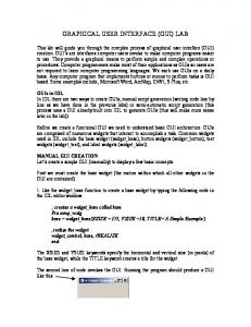
Figure 1: Example for a locally set up Shiny Server, here at the IRAMAT-CRP2A in Bordeaux. Installed are all applications available through the package ’RLumShiny’ and additional applications freely available via GitHub or CRAN. The server is accessible within the local network of the IRAMAT-CRP2A only.

cial administrator’s guide15 instead. In some cases it may also be viable to use RStudio’s self-service platform http://shinyapps.io, a hosting environment where users can easily upload, run and share their shiny applications. The service offers different subscription plans depending on the desired number of allowed applications, service availability and feature content.

usually consists of two separate panels: an input panel on the left-hand side and an output panel on right-hand side. The top of each panel contains a varying amount of tabs (depending on the app) and a context-dependent content area below. In case of the input panel the content areas include various input widgets by which the parameters of the underlying function can be manipulated. Depending on the required data type of the manipulated function parameter these widgets include buttons, checkboxes, sliders, numeric and text input fields and others. Each time the user interacts with these elements the output is automatically updated, i.e., plots are redrawn and numeric output is recalculated. The first tab of the input panel is always the ”Data”-tab, where the user is able to provide the input data. In some cases the user is also able to provide a second data set, e.g., in the application for creating abanico plots (Section 3.3.1). Input data, usually equivalent doses and their individual errors, can be provided as plain text files. Additional options allow specifying the column separator or if the first line should be treated as column headers. With respect to the output panel the first tab is always a plot, followed by one or two tabs showing an interactive table of the input data. In case of the plotting applications the last output tab shows a dynamically generated R script that can be copied to a text editor or RStudio and used to reproduce the current plot as seen in the ”Plot”-tab. We regard

3.2. Application layout and capabilities Almost all shiny applications included in the ’RLumShiny’ package follow a common layout style (Fig. 2). The exception to the rule is the application for calculating the cosmic dose rate, which will be presented separately in Section 3.3.2. The following layout descriptions hence refer to all applications other than the one for calculating the cosmic dose rate. A general characteristic all shiny applications share, however, is the responsive design, meaning that the layout adjusts dynamically while taking into account the characteristics of the device used. Shiny applications are thus always correctly rendered and perfectly usable on desktop computers, mobile phones and anything in between. Currently, each application in the ’RLumShiny’ package 15 http://docs.rstudio.com/shiny-server/, 2016-11-18.

accessed:

26


Input

TL, Vol. 34, No. 2, 2016

Output c

a

d b

e

f Figure 2: General layout of shiny applications in the ’RLumShiny’ package. The applications follow a common GUI layout with two separate panels for input (left) and output (right). Both panels consist of a header with a varying amount of tabs (a, c) and a context-depend content area (b, d). In the example shown here (app RLum(app = ’doserecovery’)) (b) shows the ”Data” tab content where the user is allowed to provide up to two data sets as an ASCII text file. Additional check boxes and radio buttons allow for providing the files in various style formats. Some of the input elements provide custom tooltips with graphical or text information (e). The ”Bookmark” button (f) below the input panel allows saving the current state of the application. The user is provided an URL, which can be used to restore the session, i.e. all previous settings and provided data are automatically restored.

this as a valuable addition as (i) users may use this as a help to understand all the arguments of a particular function and are able to see how they should be used, and (ii) it provides the means to fully reproduce the plot from the CLI or in an existing R script. Naturally, all applications for generating plots offer an export section, which is accessed by the second to last tab on the input panel (Fig. 3). There, the user is able to save the generated plot in a vector graphics format (PDF, SVG or EPS). Note that the plot dimensions in the exported file usually differ from those seen in the ”Plot”-tab, as the latter is dynamically rescaled depending on the current size of the viewport. The height and width of the exported image can be specified separately. Additionally, the user can download an R script that includes the code required to reproduce the plot from the CLI.

are to calculate the cosmic dose rate and to transform continuous-wave OSL curves to a pseudo hyperbolic, linearly or parabolic modulated curve (Table 1). In the following, specific capabilities of the ’RLumShiny’ package are exemplified by the applications for creating an abanico plot and for calculating the cosmic dose rate. 3.3.1

Abanico Plot

The abanico plot was introduced by Dietze et al. (2016), a novel plot type for showing chronometric data with individual standard errors. In essence, it is a combination of a radial plot (Galbraith, 1988) and a kernel density estimate (KDE) plot (cf. Galbraith & Roberts, 2012), which can be created using the R function Luminescence::plot AbanicoPlot(). To produce a ready-to-use plot the user only needs to provide some input data. Yet, Luminescence::plot AbanicoPlot() offers 33 arguments and an uncounted number of base R arguments that can be used to style the plot to ones desire. As plots generated in R cannot be changed after they have been drawn the user is required to repeatedly run the function call

3.3. Example applications In the current version of ’RLumShiny’ (v0.1.1) more than half of all included applications are exclusively there for creating graphical output. The remaining applications 27


TL, Vol. 34, No. 2, 2016

c a

b

Figure 3: File export options available for the histogram application (app RLum(app = ’histogram’)). All plotting applications of the R package ’RLumShiny’ include an export tab in the input panel, which (a) offers the possibility to save the generated plot as a vector graphics file (file types: PDF, SVG, EPS). Additionally, (b) the user can download an R script file that includes the code shown in in the output panel (c), which can be used to reproduce the generated plot in any other R environment that has the ’Luminescence’ package installed. Alternatively, the user can also just copy and paste the code in (c) and execute it in an R console.

c

a

e

b d

Figure 4: A selection of input options available in the shiny application to generate abanico plots. a) Mutually exclusive options such as the summary position are often manipulated using a drop down menu. b) Binary options like showing or hiding numerical information on the plot can be controlled by checkboxes. c) Plot annotations and axis labels can be changed by text input fields. d) Function arguments requiring a single numeric value or a range of values can be controlled by regular or double-ended range sliders. e) ’RLumShiny’ includes the JavaScript library JSColor (Odvarko, 2014) along with a custom ’shiny’ binding. In this example, if the user chooses ”Custom” for the datapoint colour a text input field and a colour table appears, from which a colour can be picked. Alternatively, a hexadecimal RGB value can be typed in directly.

28


TL, Vol. 34, No. 2, 2016

while iteratively changing the input parameters. Even for experienced users this may be a tedious and time-consuming task. Compared to all other shiny applications in ’RLumShiny’ the GUI for generating abanico plots offers the highest number of input widgets (Fig. 4). Generally, a numeric range (e.g., axis limits) is usually controlled with a regular or double-ended range slider, binary options (e.g., showing or hiding the summary) with checkboxes and mutually exclusive options (e.g., line type) with radio buttons or drop down menus. Text fields are mostly used to manipulate plot annotations and axis labels. The jscolorInput() function in ’RLumShiny’ extends the ’shiny’ interface by including the web colour picker JSColor16 (Odvarko, 2014). When the user chooses ”Custom” as input in one of the colour drop down menus (e.g., in the ”Datapoint”-tab) a new text input field appears. There, the user is able to enter a hexadecimal RGB value or to pick a colour from a small colour table that appears when the user clicks in the input field. 3.3.2

its layout differs from all other applications in ’RLumShiny’, and (iii) as it includes a unique feature. Despite its universal use, the equation to calculate the cosmic dose rate provided by Prescott & Hutton (1994) is falsely stated to be valid from the surface to 104 hg cm-2 (1 hg cm-2 = 100 g cm-2 ) of standard rock17 . The original expression by Barbouti & Rastin (1983) only considers the muon flux (i.e., the hard-component of the cosmic flux) and is, by their own account, only valid for depths between 10 hg cm-2 and 104 hg cm-2 . Thus, for near-surface samples (i.e., for depths