Robomote: Enabling Mobility In Sensor Networks KARTHIK DANTU MOHAMMAD RAHIMI HARDIK SHAH SANDEEP BABEL AMIT DHARIWAL and GAURAV SUKHATME Dept of Computer Science University of Southern California
Severe energy limitations, and a paucity of computation pose a set of difficult design challenges for sensor networks. Recent progress in two seemingly disparate research areas namely distributed robotics and low power embedded systems has led to the creation of mobile sensor networks. We conjecture that augmenting static sensor networks with mobile nodes addresses many design challenges that exist in static sensor networks. We present here the Robomote, a robot platform that constitutes a single node in a mobile sensor network. We conclude by listing some of the research challenges that exist in enabling large networks of such mobile sensors in reality. These include rethinking some of the decisions taken in static sensor networks and some that are new to mobile sensor networks. Categories and Subject Descriptors: H.4.0 [Information Systems Applications]: General General Terms: Sensor networks, mobile sensor networks, actuation Additional Key Words and Phrases: Robomote, mobile sensor network, sensor networks, actuation, actuated sensor networks, controlled mobility, mobility, robotics
1. INTRODUCTION Sensor networks are envisioned to revolutionize our daily life by ubiquitously monitoring our environment and/or adjusting it to suit our needs. The benefits of this technology has been elaborated at length in literature [Kahn et al. 1999; Estrin et al. 2000; Pottie and Kaiser 2000]. Here we will take a quick look at the main challenges to be overcome in enabling such technologies:
Authors’ address: Dept of Computer Science, University of Southern California, 741 W 37th Place, Los Angeles, CA 90089. Contact email:
[email protected] Permission to make digital/hard copy of all or part of this material without fee for personal or classroom use provided that the copies are not made or distributed for profit or commercial advantage, the ACM copyright/server notice, the title of the publication, and its date appear, and notice is given that copying is by permission of the ACM, Inc. To copy otherwise, to republish, to post on servers, or to redistribute to lists requires prior specific permission and/or a fee. c 2004 ACM 0000-0000/2004/0000-0001 $5.00
ACM Journal Name, Vol. 1, No. 1, 12 2004, Pages 1–0??.
2
·
Enabling Mobility in Sensor Networks(Working Paper)
1.1 Low Power consumption Sensor networks have limited energy storage. Even if they are rechargeable, they need to conserve energy for periods when energy is scarce (e.g.: nighttime for solarpowered nodes). Hence, energy efficiency is always a design constraint in sensor networks. Since decay of energy and death of some nodes are a given, it is important that the applications display graceful degradation of behavior as the energy in the network depletes. Techniques to harvest energy from the environment could also be embedded into the applications. 1.2 Limited Resources Since these nodes are small in size and need to be very cheap, the amount of computational power and other resources that can be put on a single node is also constrained. E.g: The Berkeley mote [Hill et al. 2000] has a 4 Mhz processor and 8k RAM in comparison with a 1 Ghz and 512 MB RAM in a reasonable desktop system. 1.3 Highly distributed As mentioned earlier, such networks are pictured to be deployed in large numbers. They can be thought of as highly distributed systems. It is important that all designs are scalable. Since the available resources on any given node is minimal, the strength of such networks is in the numbers. They are deployed in thousands and require use of massively distributed algorithms to function most optimally. It has been noted that Adaptive Fidelity[Intanagonwiwat et al. 2000] is a key characteristic for algorithms designed for such systems. Another important suggestion for scalability is the use of Localized Algorithms [Estrin et al. 1999]. 1.4 Deployment and Coverage One of the initial challenges to use large sensor networks is deployment. The main design goal of deployment is the effectiveness of the functioning of a sensor network . Since the number of nodes being deployed is very high, it is difficult to carefully handplace each of the nodes. At the same time, we want these nodes deployed strategically such that they sense most number of events. This might imply covering most area in the region of deployment or provide certain densities in certain regions which have a higher probability of event occurance. 1.5 Need for Calibration To deploy such sensor nodes in large numbers, it is implied by cost that the sensors be available cheaply. An effect of this is that errors are inherent in such sensors. It is important to put in place a method of distributed calibration to be able to coarsely calibrate these sensors periodically. Also, the use of probabilistic techniques to correct/adapt to some degree of error helps develop more robust algorithms. 1.6 Basic System Services Apart from being deployed, there are a set of systems services that must be implemented for the sensor network to function in a coherent manner. Some of them are listed below: ACM Journal Name, Vol. 1, No. 1, 12 2004.
Karthik Dantu et al.
·
3
1.6.1 Localization:. Each node should be able to approximate its location either globally or locally. This helps in identifying what peice of the environment that node is sampling. 1.6.2 Time Synchronization:. Since the sensors mostly produce time-series data, it is important that all nodes in the network be synchronized on time scale. 1.6.3 Routing:. Most of the times, these sensor nodes are deployed in an adhoc fashion. Upon deployment, they need to figure a good routing scheme to efficiently and reliably transport data sensed from different parts of the network to a central place from which this data can be sucked out. 1.7 Network Dynamics Variation in communication range, frequent death of nodes due to lack of energy and other environmental causes result in large variations in network topology. Given that network dynamics are an integral part of such networks, applications should be able to adapt gracefully to variations in the network topology. 1.8 Spatio-Temporal Irregularity Studies show that there exists irregularity in sampling in both space and time in sensor networks. [Ganesan et al. 2003] consider two casestudies to show the impact of spatio-temporal irregularity in sampling. They also suggest some corrective strategies but acknowledge that such irregularities are inherent in static sensor networks. 1.9 Data-centric Naming There is a fundamental difference in the type of data requested from such networks [Heidemann et al. 2001]. More often than not, aggregates of the data are of more interest rather than the readings of one particular node. Due to the unreliable nature of the sensors and the limited computational capability of such nodes, aggregate values are also better indicators and would be closer to the real value. This leads to the data-centric paradigm where we name the data as opposed to the nodes. 1.10 Concurrency intensive It is suggested [Hill et al. 2000] that such sensor networks are concurrency intensive. Such networks see lot of traffic when an event is detected but might not see any activity for long periods between events. Many parallel processes would be needed to handle data at times of high load. One of the design goals of TinyOS has been to incorporate concurrency by providing lightweight threads [TinyOS ]. 2. WHY MOBILITY? Controlled mobility enables a whole new set of possibilities in sensor networks. The ability of actively changing location can be used to mitigate/solve many of the design challenges outlined above. Before we look at some of the advantages, we would like to clarify that controlled or robotic mobility is different to mobility in the context of the term in Mobile Adhoc Networks (MANETs). MANET studies consider mobility as a given. They study the effects of mobility and assume no ACM Journal Name, Vol. 1, No. 1, 12 2004.
4
·
Enabling Mobility in Sensor Networks(Working Paper)
control over it. However, controlled or robotic mobility is the ability to move intentionally. It enables many possibilities and also has an energy cost to be paid. We outline some of advantages of controlled mobility below: 2.1 Deployment Controlled mobility can be used to place sensors at the optimal places for monitoring. It is conceivable in networks that are fully mobile or consist of a mixture of static and mobile sensors that the mobile nodes align themselves such that the deployment is optimal to monitor events under consideration. An algorithm for deploying a fully mobile sensor network has been proposed [Howard et al. 2002]. We could conceive of a family of algorithms for deployments that have varying ratios of static to mobile sensor nodes that optimize various metrics like maximum coverage, required connectivity [Poduri and Sukhatme 2004] etc. 2.2
Adaptive Sampling
One of the fundamental requirements from a sensor network is to sample its environment. As pointed out in Section [1.8], static sensor networks have been shown to exhibit spatio-temporal irregularity in sampling. This gives rise to many design problems. Controlled mobility can be used to alleviate this issue to an extent. It is possible to think of adaptive sampling strategies where spatial adaptation is by the use of mobility. Temporal irregularity however needs more complex mechanisms to correct and is an open research problem. 2.3
Network Repair
One of the main problems of adhoc deployment is the lack of guarentee of connectivity (or a certain level of connectivity) in the network. If part of a network gets disconnected because of nodes dying, there is little that can be done to repair it. However, such situations can be corrected by having a few mobile nodes which can actively move to desired locations and repair broken networks. 2.4
Energy Harvesting
Methods have been suggested [Rahimi et al. 2003] to use mobile sensor nodes to physically transport energy in the network from areas where they are available in plenty to other regions where energy availability is scarce. This work [Rahimi et al. 2003] indicates the possibility of self-sustaining networks in the presence of some constant source of energy (like solar energy) using mobile sensor networks. 2.5 Localization Localization has been identified as one of the fundamental systems services essential for proper functioning as a sensor network [Savvides et al. 2001]. Localization has also been one of the fundamental problems of study in distributed robotics [Thrun et al. 2001] [Thrun et al. 2000]. With the augmentation of static sensor networks with some mobile nodes, it is possible for us to incorporate some of the algorithms developed in distributed robotics for localization of mobile nodes. We can also conjecture hybrid algorithms that make use of both static and mobile sensor nodes in a symbiotic fashion. ACM Journal Name, Vol. 1, No. 1, 12 2004.
Karthik Dantu et al.
·
5
2.6 Event Detection As mentioned in Section[1.4] event detection is one of the fundamental functions of a sensor network. Also, events are usually not evenly distributed in space. Hence, the initial deployment might not be the optimal deployment of nodes to detect events in time. We can correct this problem by having mobile nodes that move to regions of high probability of event detection over time. This arrangement could also be dynamic with mobile nodes repositioning themselves as and when required. 3. ROBOMOTE: AN EXAMPLE PLATFORM FOR MOBILE SENSOR NETWORKS 3.1 Introduction The Robomote [Sibley et al. 2002] was designed to be a tabletop platform for experiments on a testbed. The primary design goals for the robomote were two fold : (1) Ease of Deployment (2) Cost
Keeping these in mind, compatibility with the Berkeley mote [Hill et al. 2000] was an obvious choice. We present here the second revision of the robomote Fig.[3.1]. The Robomote consists of an Atmel 8535 microcontroller [Atmel ]. This is a 8bit AVR RISC MCU with 8k bytes of In-system programmable flash alongwith 512 bytes of EEPROM and 512 bytes of Internal SRAM. The microcontroller also incorporates various desirable features like programmable sleep modes and reprogramming capability. It has two motors [Micromo ], a compass for bearing [Honeywell ] and IR bump sensors [Panasonic a] [Panasonic b]. Each of these are described in more detail below. The robomote is complete with the addition of a Berkeley mote[Hill et al. 2000]. The mote is used as the master and all basic functionality of the robomote are exported to the mote via modular interfaces. We have also written TinyOS components for the mote to incorporate control of the robomote into ACM Journal Name, Vol. 1, No. 1, 12 2004.
6
·
Enabling Mobility in Sensor Networks(Working Paper)
TinyOS apps. Just as the mote has a radio component and can send out packets, it now has an actuation component and can physically actuate at will . For convinience, we call the robomote as the lower layer and the mote the upper layer. Each of the components of robomote are elaborated at greater detail below. 3.2 Hardware Architecture 3.2.1 Communication:. Communication between the robomote and the mote is via a serial interface and can achieve speeds of upto 19.2 kbps. There is a byteto-byte reliability established via acknowledgements from the lower layer for every byte received. This helps detect loss of commands and/or data. Each command consists of two bytes - a command and corresponding data. Some commands do not have any data to be passed and are padded (eg: get bearing of the compass). 3.2.2 Motion Control:. The wheels have DC motors from Micromo [Micromo ]. The nominal voltage of the motors is 6 volts and the output power is 1.41 Watts. The efficiency of the motors is 71% with a no-load speed of 16,300 rpm and a noload current of 30 mA. The motors are controlled using an H-bridge, made from discrete components, and utilizes Pulse Width Modulation ( PWM ) for its operation. The four signals which control the motors are PWM1, PWM2, Direction1 and Direction2. By changing the direction bits, the direction of the motors can be reversed. Motion control is triggered by velocity and distance commands from the upper layer. These commands are converted to the corresponding PWM and tick values. The gear ratio is 25:1. The robomote relies on precise odometry for movement from one location to another. The feedback uses IR TX/RX mechanism for sensing the number of ticks on the wheel. Every rotation of the motor shaft produces 6 ticks, which are then processed by the op-amps. Hence, for every revolution of the wheel, we get 150 ticks for feedback control. This is then fed back to the counters of the Atmel Microcontroller. The robomote implements a PI-controller that corrects for odometry error inherent in the motors and attempts to run the robomote straight. The PI-controller is activated with a frequency of 2 Hz. It computes the difference in ticks between the left and right wheels and feeds corrections back to the PWM inputs that are applied to the motors.The controller is bypassed for turn commands and calibration to avoid additional complexity. 3.2.3 Compass:. The compass on the robomote is a 2-axis Honeywell HMC1022 IC. It is configured as a 4-element Wheatstone bridge. These magneto-resistive sensors convert magnetic fields to differential output voltage. From this two analog readings are obtained, one that senses the Earth’s North-South and another at 90 degrees to the first (i.e. West-East readings). The sensors are not absolute and must be calibrated at robot initialization and periodically throughout usage. This is done by entering a calibration phase where the robomote makes a full turn to detect the max and min readings and sets them as reference. The compass can be run in two modes ACM Journal Name, Vol. 1, No. 1, 12 2004.
Karthik Dantu et al.
·
7
—free-running mode —single conversion mode. We use it in a single conversion mode to conserve energy avoid usage of the compass when not required. When a request for compass reading is obtained from the upper board, charge is passed to the compass. This causes the compass to get activated and the azimuth reading is obtained which is then passed on to the upper layer. 3.2.4 IR Bump Sensors:. Robomote has two infra-red transmitters [Panasonic b] and one receiver [Panasonic a] respectively on either side. The transmitters produce 940nm wavelength which are modulated at 40 KHz over 1.5 KHz in order to reject the maximum amount of ambient light. The receiver has a viewing angle of 40 degrees with 80% sensitivity. The receivers can be selected by using a multiplexer and an interrupt is generated on the controller’s external interrupt channel. These sensors are used to detect obstacles in the path of motion of the robomote. Obstacle avoidance runs in the free-running mode. There is a threshold value for the IR receiver and if it detects IR signals above it, the upper layer is signalled warning it of obstacles. 3.2.5 Rechargeable Battery:. The robomote is provided with a rechargeable Lithium Ion battery [Renata ]. The battery can be charged by either by solar energy or by DC wall charger. The wall charger uses LTC1734 chip from Linear Technologies [Linear b]. The solar charger uses the LTC1734L from Linear technology [Linear a]. For the Solar charger, the minimum current supplied to the battery is 50mA, and it can be increased by a NV trimmer potentiometer(DS1804). The battery itself is a Li-Ion prismatic rechargeable battery, from RENATA [Renata ]. The typical capacity of the battery is 345mAh and it has a nominal voltage range of 3.7V. The weight of the battery is 10.1g.
Fig. 1.
A group of robomotes
3.2.6 Energy Consumption:. We have measured the energy consumptions of the individual components of the robomote. The energy profile is shown in Fig.[2]. ACM Journal Name, Vol. 1, No. 1, 12 2004.
8
·
Enabling Mobility in Sensor Networks(Working Paper)
Fig. 2.
Power consumption percentage of various peripherals for the robomote
Table I. Power Consumption of Peripherals COMPONENT POWER CONSUMPTION (in watts) Both Motors On Compass IR (Both IR TX/RX On) Both LEDs All external services off (MCU + MOTE VDD + Leakage)
0.72 0.06 0.588 0.044 0.036
3.2.7 Energy utility Tradeoff:. It is interesting to compare this with the power consumption of the MICA mote as seen in [Mainwaring et al. 2002]. Note that actuation (physical movement) draws much more energy than computation or communication(Fig.[2]). Hence, the energy consumption in increasing order of consumption seems to be Computation < Sensing < Communication < Actuation. This is an important design consideration to keep in mind while designing algorithms for mobile sensor networks. 3.3 System Architecture 3.3.1 Actuation. The main feature of an actuator system is its ability to move. This is facilitated by wheels that are run by motors. However, precise control of the motors is very difficult. Odometry error is a well-known problem and has been observed at length in robotics [Jones et al. 1998]. It arises from many factors like slipping and error in motor control. One solution to alleviate this problem is incorporation of a feedback controller that continually corrects for the error in odometry. Considering that these actuator nodes have to be cheap, some feedback mechanism must be present to acheive any reliable actuation. ACM Journal Name, Vol. 1, No. 1, 12 2004.
Karthik Dantu et al.
·
9
Sensor Board
Mote
Serial
Encoders
Motors
Fig. 3.
Fig. 4.
count ticks
Atmel 8535
Apply Feedback
IR Sensor
Compass
System Architecture of robomote
System Architecture of the Pioneers [ActivMedia a]
ACM Journal Name, Vol. 1, No. 1, 12 2004.
10
·
Enabling Mobility in Sensor Networks(Working Paper)
command Robomote.Move(uint8 t distance) Move straight for distance cm. command Robomote.Turn(uint8 t angle, uint8 t direction) Turn relative to current position in anti−clockwise(direction=1)/clockwise(direction=0) by angle degrees. command Robomote.ATurn(uint8 t angle) Turn to absolute position angle degrees. event result t Robomote.MoveDone() Signify completion of the move command. event result t Robomote.TurnDone() Signify completion of the turn command. event result t Robomote.ATurnDone() Signify completion of the absolute turn command.
Fig. 5.
Actuation Interface provided by robomote
The robomote has optical encoders that produce 150 ticks per revolution of the wheel. This is much more coarse than the Khepera that produces about 600 ticks. The robomote design of feedback control is similar to that of the pioneers([ActivMedia b], Fig.[3], Fig.[4]Table[III]). As mentioned in Section 3.2.2, we have implemented a PI controller to correct for odometry error so that the robomote drives straight. The other enhancement has been that we have moved away from a polling mechanism to keep track of distance traveled. We have now wired the ticks to one of the asynchronous counters of the processor and an interrupt is signalled. Since counting the encoders and applying corrections have to be done at the finest resolution possible, this functionality resides very close to the motors in both cases. There is a specialized board in case of the pioneers that performs the PIDcontrol. The robomote also has a separate processor (Atmel 8535) for this purpose. This processor also performs the task of reading the IR sensors, the compass and communicating with the mote. All other functionality other than feedback control is handled by the upper layer. The lower layer just acts as the interface for the devices. Actuation is supported on the mote via three simple commands as shown. Each of the commands results in an event to notify the completion of the command. Note that the split-phase methodology that is present in other component interactions in TinyOS has been maintained [Levis et al. 2004]. As elaborated in [Levis et al. 2004] this model is a good way of maintaining high concurrency with low state. ACM Journal Name, Vol. 1, No. 1, 12 2004.
Karthik Dantu et al.
·
11
command result t Compass.calibrate() event result t Compass.calibrateDone() command result t Compass.getData() event result t Compass.dataDone(uint8 t azimuth) command result t IR.enableObstacleAvoidance()
Fig. 6.
IR sensors and Compass Interface
3.3.2 Sensors on Lower Board:. There are two other sensors on the lower board as shown in Fig.[3]. One of them is two sets of IR bump sensors (each consisting of two IR Transmitters and one IR receiver). The other is the compass. We have changed the access mechanism for the compass from free-running mode (in Robomote version 1) to single conversion. This saves energy by not querying the compass when it is not being used. 3.4 Software Architecture As mentioned earlier, we intend to use the mote as the master. Hence, the system software on the robomote has been designed to provide the basic functionality as modules on the mote. We have designed modules in TinyOS to allow easy access to robomote’s functionality in TinyOS. The TinyOS modules consist of two layers. There is a Hardware Abstraction Layer that takes care of the communication with the robomote. The second layer exposes the functionality of each individual feature (e.g.: compass) of the robomote to applications in TinyOS. It is possible to include just the required components into existing TinyOS apps for ease of understanding and clear design. This is illustrated better in Fig.7. 3.5 Testbed Setup Our setup includes a testbed [Rahimi et al. 2002] with beacons at known locations. Using these, we have a coarse localization implemented (based on triangulation). There is also an Orientation component that combines the Compass with the localization to get relative bearing on which direction to go next, given a destination. We have written a higher level Navigation component that performs the task of navigating from point A to point B using this localization and orientation. 4. ENHANCEMENTS IN ROBOMOTE VERSION 2 This is version 2 of the robomote. Many features have been improved from the first version [Sibley et al. 2002]. Some of them have been illustrated in the table above. One of the biggest challenges has been accurate motion control. As elaborated in Section 3.3, we have incorporated feedback control for the same. Reliability has been improved by providing for acknowledgements for command and data bytes being exchanged between the mote and the robomote. Last, but not least, we have ACM Journal Name, Vol. 1, No. 1, 12 2004.
12
·
Enabling Mobility in Sensor Networks(Working Paper)
Fig. 7.
FEATURE
Block Diagram of Software components
Table II. Robomote v1 v/s v2 ROBOMOTE v1 ROBOMOTE v2
Gear Ratio Encoders for wheels PI Control for wheels Battery Battery Lifetime Charge time for battery Odometry Compass
20:1 No No Li-Ion 10-15 mins 1.5 hours Polling Free running
25:1 Yes Yes Li-Ion Prismatic 30 mins 20 minutes Interrupt-based Single Conversion
incorporated a better rechargeable battery which has a shorter recharge cycle and longer life. Energy saving has been brought about by switching from free running mode to single conversion mode. 5. COMPARISON WITH OTHER POPULAR ROBOTIC PLATFORMS We compare the robomote with popular actuator platforms just to show the space within which the robomote fits. One feature that stands out with regard to mobility in all these platforms is the need for feedback control. This has been elaborated before in Section 3.3. Note also that since this form of error correction needs to be performed very frequently, the sensors used for feedback control are tied in much closer to processing than the other sensors (Figures [4][3]). ACM Journal Name, Vol. 1, No. 1, 12 2004.
Karthik Dantu et al.
·
13
The other major distinction we would want to make is the fact that robomote is a small robot. It is not intended to traverse terrains and encompass the functionality that some of the bigger robots possess. It has been designed to work with motes and provide mobility in a sensor network setup. A more detailed comparison is given in Table[III]. Table III. Parameter
Hardware comparison with other popular robotic platforms Robomote
Khepera
Pioneer 3-DX
heli
Length:380 mm Width: 440 mm Height: 220 mm 9 kg 23kg
Length: 1570mm Width: 620 mm Height: 770 mm 8.18 kg 10kg
12-V lead-acid battery
Liquid Fuel Gas and Two-stroke oil 4050mAh 30-40 mins N/A
PHYSICAL Length: 70mm Width: 45mm Height: 35mm 85g-90g 300g
Diameter: 70mm Width: N/A Height: 30mm 80g 250g
Total Power draw Run time Recharge time
Rechargeable Battery 345mAh 20-30 mins 20 mins
3 AA Rechargeable Ni-MH batteries Not known 1hr 6 hrs
Steering Error Correction Gear Ratio Linear Speed Wheel Diameter Turn Radius Traversible Terrains
Differential PI-controller 25:1 15-20 cm/s 1.5 cm 5 cm Tabletop
Differential PID Control unknown 1 m/s 1.5 cm
On-board Computing
Atmel 8535
Motorola 68331
PC-104 Stack
Communication On-board Storage
Wireless, UART 4k EEPROM
Reprogramming On-board Sensors
Serial (as of now) IR bump sensors
Serial, Radio board 512K Flash 8k Flash Serial IR proximity sensors
Compass optical Encoders sensor board
Gripper Video Module Radio-T
802.11b Hard disk or Compact Flash N/A Sonar ring (front and rear) GPS Laser-range finder
Dimensions Weight Payload
POWER Type of Fuel
18-24 hrs 12 hrs
MOBILITY
Tabletop
Differential PID Control 36:1 1.2 m/s 19 cm In place Wheelchair accessible
N/A PID Control N/A 20 m/s N/A In place N/A
ON-BOARD ELECTRONICS 1 PC-104 Stack(vision) 1 PC-104 Stack (control) 802.11b Compact Flash N/A GPS, Compass IMU (3 Gyros and accelerometers) 2 sideways cameras 1 omnicam 1 downward looking camera Laser-range finder
6. CASE STUDIES - EXPERIMENTS USING THE ROBOMOTE AS A MOBILE SENSOR NODE 6.1 Detecting Level Sets of Scalar Fields using Mobile Sensor Networks 6.1.1 Problem:. Assuming that there is a static sensor network deployed in a bounded area, the problem is that of detecting level sets(contours) of the sensed ACM Journal Name, Vol. 1, No. 1, 12 2004.
14
·
Enabling Mobility in Sensor Networks(Working Paper)
Table IV. Experimental results on the robomote Optimal Distance Traveled Distance Ratio 5.5 8.3 1.509 5 6.1 1.22 5 7.6 1.52 3 5.5 1.83 5 7.8 1.56
scalar field (Eg: Isobars for pressure, isotherms for temperature) using a mobile sensor node. This could be visualized to be a mechanism for event detection. It is also a classic example where mobile sensor nodes could augment static sensor networks to perform tasks not possible otherwise. 6.1.2 Algorithm:. The idea is to perform gradient descent on the sensed scalar field. We use a control law proposed in the context of sensor-based path planning [Choset et al. 1997] for this purpose. The control law has been adapted for the sensor network case. Simulation results show that the percentage of success of detecting the desired level set goes to above 80% for node degrees greater than 7-8 of the static sensor network. This is logical since network connectivity might not exist for networks below node degree 6 [Xue and Kumar 2003]. 6.1.3 Experiments:. We performed experiments on our testbed [Rahimi et al. 2002]. This was to validate the algorithm in the presence of odometry error. The experiments consisted of a matlab setup on a PC that simulated node deployment. The robomote would query the PC to read the sensor readings of its immediate neighbors. Based on it, motion control commands were generated in matlab for gradient descent. This would be executed by the robomote on the experimental testbed. This would iterate until the robomote reached the desired contour. The results validate the optimality results of our simulations. Twenty nodes were deployed in a 4ft by 8 ft area and radio range was about 2.8 feet. We performed the experiment for 10 different types of deployment and four start positions. Node degree was 8. The gradient simulated is a simple linearly decaying gradient. The ratio of traveled distance to optimal is about 1.4. Success percentage for these trials were between 75% and 80%. 6.2 Bacteria inspired robots for envirnmental monitoring 6.2.1 Overview/Experiment Motivation:. The problem at hand is to locate and track a light source using the photo gradient generated by it over time using mobile sensor nodes (robomote) on the table top test bed. We implement an algorithm based on biased random walk, modeled on taxis in bacteria [Berg 1983], for tracking gradient sources. Using gradient information and rudimentary motion strategy, the mobile senor nodes are able to track gradient sources analogous to the manner in which bacteria detect and track potential food sources using the gradient generated by the food sources and simplistic locomotion strategies. The strategy of such a bacteria-like node can be summarized as ”sense and move”. For a more detailed description of the algorithm, the reader is referred to [Dhariwal et al. 2004]. ACM Journal Name, Vol. 1, No. 1, 12 2004.
Karthik Dantu et al.
Fig. 8.
·
15
Robomote with the Sensor
A mobile sensor-node executing a biased random walk has very little requirements in terms of memory since only the last sensor reading needs to be stored. The processing requirements are minimal since the only processing required is comparison between successive sensor readings (gradient computation). Only a minimal amount of motion control is required to hold the heading of the robot in a particular direction for a particular duration of time (depending on bias levels). All these characteristics make the robomote an ideal platform to carry out our experimental work. In this case study, we focus on a 2D version of the gradient detection and source tracking problem, and evaluate the results we obtained in simulation [Dhariwal et al. 2004] on the robomote platform. 6.2.2 Experiments with ROBOMOTE as the mobile sensor node:. We carried out experiments on the robomote to validate our simulation results on actual mobile sensor nodes executing a biased random walk. We used a mica mote to provide the control commands to the robomote using TinyOS. We used the two basic components move and rotate for controlling the robomote to carry out the biased random walk. We used a basic sensor board with a photo (light) sensor that could sense the light gradient generated by the light source. The experimental setup can be seen in Fig.[8]. The position of the robomote on the test bed was tracked using an overhead vision system which captured image frames and passed these to a tracker [Howard 2002] for data analysis and storage. Color blobs mounted on top of the robomote helped track its position over time on the table top test-bed. 6.2.3 lows:
THE RANDOM WALK ALGORITHM:. The algorithm proceeded as fol-
(1) Record the current photo intensity reading from the photo sensor P(i) (2) Move along a straight line for a distance equal to the mean free path of the experiment (3) Record the current photo intensity reading from the photo sensor P(i+1) (4) If the difference P(i+1) - P(i) > 0, move along the same direction for a distance proportional to the bias factor for the experiment (5) If goal reached, then (a) stop ACM Journal Name, Vol. 1, No. 1, 12 2004.
16
·
Enabling Mobility in Sensor Networks(Working Paper)
Fig. 9.
Fig. 10.
Light Gradient
The percentage gradient
(b) else rotate by a random angle and go back to step 1 The robomote is mounted with a light sensor as shown in Fig.[8]. We begin by setting up a photo gradient generated by a light source placed at one end of the robomote test bed as shown in the Fig.[9]. The robomote is then positioned on a circular arc of radius d (d = 40cms.) units from the center of the light source, generating the photo gradient, on the table. The heading and position of the robomote on the arc was a random variable and could be towards or away from the source. A smaller circular arc of radius D (D=5cms.) units from the center of the light source was marked as the goal for the robomote. The robomote was switched on at distance d, and tracked as it performed a biased random walk on the table following the photo gradient. The experiment terminates when the robot reaches the smaller circular arc of radius D. The speed of the robomote was set at 2cm/s. for the experiments. The experiment was repeated for several other values of starting distance d (d = 80cm, 120cm). We repeated the experiment 75 times for each of the d values with random starting orientations and locations on the arc and averaged our position readings between the gathered data for our analysis. We believe this was a fair set of samples to evaluate the effectiveness of the approach. The graphs for the metrics proposed in the [Dhariwal et al. 2004] can be seen in Fig.[11]. The results from the robomote platform agree with the results obtained from the simulation work presented in [Dhariwal et al. 2004] ACM Journal Name, Vol. 1, No. 1, 12 2004.
Karthik Dantu et al. 110
·
17
Robomote Simulation
100 90
Distance from Source −>
80 70 60 50 40 30 20 10 0
0
100
200
Fig. 11.
300
400 Time −>
500
600
700
800
Robomote with the Sensor
150 140 130 120
Distance from Source −>
110 100 Source 1 Source 2
90 80 70 60 50 40 30 20 10 0
0
100
200
300
Fig. 12.
400
500
600
700 800 Time −>
900
1000 1100 1200 1300 1400 1500
Robomote with the Sensor
We carried out another set of experiment with two equal intensity sources present at the same time at opposite corners of the test bed and started the robomote at distances d (d = 25%,50%(center) and 75% positions on the test bed)Fig.[10]. We started with only one source switched on initially at t = 0s. At t = 180s. we switched on the second source located at the other end of the test bed. This was followed by switching off the first source completely at t=435s. We repeated the experiment for the different values of d (d = 25%,50%(center) and 75% positions on the test bed)). Again the results (Fig.[12]) obtained in hardware platform were in agreement with our simulation results. 6.2.4 Conclusion:. The above case studies demonstrate that the robomote platform provides an ideal test bed for implementing and testing our algorithms and verification of our simulation work for using mobile sensor nodes. The robomote platform is well suited for our work since it provides us with the essential navigation components for performing simple experiments like random walks and gradient descent. Additionally, it provides us with a set of control capabilities in terms of robot speed, direction of motion and a set of sensing capabilities which can be plugged in using add-on sensor board. ACM Journal Name, Vol. 1, No. 1, 12 2004.
18
·
Enabling Mobility in Sensor Networks(Working Paper)
7. CHALLENGES IN ENABLING MOBILE SENSOR NETWORKS We will now attempt to summarize the research issues to be solved before we can make mobile sensor networks a reality. 7.1 Robotics Issues 7.1.1 Adaptive Localization: . The most fundamental research problem in robotics is for the robot to find out where it is. There has been a lot of research in the area of probabilistic localization in robotics off late [Thrun et al. 2001] [Thrun et al. 2000]. Most of these schemes tend to be centralized and computationally very expensive. However, adding mobile nodes to static sensor networks gives us the oppurtunity of using odometry to do coarse localization and adapt some of these techniques. There is scope for research in devising less computationally intensive algorithms to suit sensor network applications. It is also important that such algorithms be distributed unlike the ones proposed in the robotics scenario. 7.1.2 Distributed Mapping: . The other important problem in robotics is to find out what is around the robot. i.e. to map the environment in which the robot is placed. However, most proposed techniques are again very intensive and rarely make use of information from more than one robots. Augmenting this information with sensor information from the static sensor network makes for an interesting study. 7.1.3 Coverage:. Coverage is an important feature of sensor networks. There has been some study in using sensor networks to maximize coverage [Batalin and Sukhatme 2003]. This work is a clear example of cooperation between mobile and static sensor nodes to alleviate problems (in this case, coverage) in sensor networks. However, there hasnt been much work on looking at mobile sensor networks and how they could be used to adapt networks by varying the coverage dynamically. 7.2 Systems Issues 7.2.1 Massive Reprogramming:. One of the requirements of a sensor network is the ability to do massive reprogramming. When thousands of nodes are to be deployed, it is infeasible to program each one by hand. However, it is possible to envision a mobile node covering the network and reprogamming all nodes that come within its range. This could be considered an instance of a multi-robot task allocation problem. 7.2.2 Distributed Calibration:. Another hard problem in sensor networks is that of calibration. Such sensors are cheap and reasonably erroneous. They require frequent calibration. We can think of having a calibrated sensor on a mobile node and the mobile node covering the area of sensor node deployment calibrating the nodes in its neighborhood. 7.2.3 Network Repair:. An interesting area of work is that of network repair. As mentioned earlier, it can be imagined that a few mobile nodes can be used to repair static networks by positioning themselves at hotspots or points of disconnection. However, moving the mobile nodes expends energy and there is scope for study of the tradeoff. This also makes for interesting theoretical study for optimal algorithms ACM Journal Name, Vol. 1, No. 1, 12 2004.
Karthik Dantu et al.
·
19
to move the mobile nodes. 7.2.4 Distributed storage,aggregation and querying techniques:. Most of the studies on data-centric storage, aggregation and querying have been w.r.t. static sensor networks. They make assumptions that might not hold good in mobile sensor networks. An example would be the data-centric storage scheme’s dependency [Ratnasamy et al. 2003] on location. The scheme employs a hash that attempts to distribute data evenly across the geography of the network. However, if there are a reasonable percentage of mobile nodes, data would have to be transfered from nodes that move to nodes that are in that geographic location. This is clearly undesirable. This calls for a revisit to services like data-centric storage for networks that have a combination of mobile and static nodes. It is important to build a model that is independent of geographic location. 8. CONCLUSIONS In summary, there are a wealth of issues that need to be looked at to enable mobility in sensor networks. We have highlighted the benefits of augmenting static sensor networks with mobility. We presented the Robomote, an example testbed platform for mobile sensor network experiments. We also presented a couple of case studies where robomote is being used to experimentally validate algorithms designed for next generation mobile sensor networks. Finally, we looked at some of the potential issues that need to be resolved in order to enable mobility in sensor networks. REFERENCES ActivMedia. Pioneer 3- and 2-h8 plus operations manual. http : //robots.activmedia.com/docs/alld ocs/P 3 − P 2H8OpM an3.pdf . ActivMedia. Technical specs of pioneer robot family. http : //www.activrobots.com/ROBOT S/specs.html. Atmel. Atmel datasheet (8535). http : //www.atmel.com/dyn/resources/prod d ocuments/DOC1041.P DF . Batalin, M. and Sukhatme, G. S. 2003. Coverage, exploration and deployment by a mobile robot and communication network. In Proceedings of the 2nd International Workshop on Information Processing in Sensor Networks. Palo Alto Research Center (PARC) Palo Alto, CA, USA, 376–391. Berg, H. C. 1983. Random Walks in Biology. Princeton University Press. Choset, H., Konukseven, I., and Rizzi, A. 1997. Sensor based planing: A control law for generating the generalized voronoi graph. In IEEE International Conference in Advanced Robotics. Dhariwal, A., Sukhatme, G. S., and Requicha, A. A. 2004. Bacterium-inspired robots for environmental monitoring. In IEEE International Conference on Robotics and Automation. Estrin, D., Govindan, R., and Heidemann, J. 2000. Embedding the Internet. Communications of the ACM 43, 5 (May), 39–41. (special issue guest editors). Estrin, D., Govindan, R., Heidemann, J., and Kumar, S. 1999. Next century challenges: Scalable coordination in sensor networks. In ACM Conference on Mobile Computing and Networking. Seattle, WA, USA. Ganesan, D., Ratnasamy, S., Wang, H., and Estrin, D. 2003. Coping with irregular spatiotemporal sampling in sensor networks. In 2nd Workshop on Hot Topics in Networks. Heidemann, J., Silva, F., Intanagonwiwat, C., Govindan, R., Estrin, D., and Ganesan, D. 2001. Building efficient wireless sensor networks with low-level naming. In Proceedings of the Symposium on Operating Systems Principles. ACM, Chateau Lake Louise, Banff, Alberta, Canada, 146–159. ACM Journal Name, Vol. 1, No. 1, 12 2004.
20
·
Enabling Mobility in Sensor Networks(Working Paper)
Hill, J., Szewczyk, R., Woo, A., Hollar, S., Culler, D., and Pister, K. 2000. System architecture directions for networked sensors. In Proceedings of Architectural Support for Programming Languages and Operating Systems-IX. ACM, Cambridge, MA, USA. Honeywell. Honeywell hmc 1022 compass chip datasheet. http : //www.ssec.honeywell.com/magnetic/datasheets/hmc1001 − 2.pdf . Howard, A. 2002. Mezzanine user manual. Tech. Rep. IRIS-02-416, Institute of Robotics and Intelligent Systems. Howard, A., Mataric, M., and Sukhatme, G. S. 2002. Self-deployment algorithm for mobile sensor networks. Autonomous Robots - Special Issue on Intelligent Embedded Systems 13, 2, 113–126. Intanagonwiwat, C., Govindan, R., and Estrin, D. 2000. Directed diffusion: A scalable and robust communication paradigm for sensor networks. In In Proceedings of the Sixth Annual International Conference on Mobile Computing and Networking. Boston, MA, USA. Jones, J., Seiger, B., and Flynn, A. 1998. Mobile Robots: Inspiration to Implementation. A. K. Peters Ltd. Kahn, J., Katz, R., and Pister, K. 1999. Next century challenges: Mobile networking for ’smart dust’. In Proceedings of Mobile Computing and Networking. ACM, Seattle, WA, USA. Levis, P., Madden, S., Gay, D., Polastre, J., Schezwyk, R., Woo, A., Brewer, E., and Culler, D. 2004. The emergence of networking abstractions and techniques in tinyos. In In Proceedings of the First USENIX/ACM Symposium on Networked Systems Design and Implementation (NSDI 2004). ACM, San Francisco, CA, USA. Linear. Linear solar charger chip (ltc1734l) datasheet. http : //www.linear.com/pdf /1734lf.pdf . Linear. Linear wall-charger chip (ltc1734) datasheet. http : //www.linear.com/pdf /1734f s.pdf . Mainwaring, A., Polastre, J., Szewczyk, R., Culler, D., and Anderson, J. 2002. Wireless sensor networks for habitat monitoring. In ACM International Workshop on Wireless Sensor Networks and Applications. Atlanta GA, USA. Micromo. Micromo motor datasheet. http : //www.micromo.com/library/docs/products/1319 S .P DF . Panasonic. Ir receiver datasheet. http : //rocky.digikey.com/W ebLib/P anasonic/W ebdata/P N A4611M Series.pdf . Panasonic. Ir transmitter datasheet. http : //www.semicon.panasonic.co.jp/ds/eng/SHC00011AED.pdf . Poduri, S. and Sukhatme, G. 2004. Constrained coverage for mobile sensor networks. In Proceedings of the IEEE International Conference on Robotics and Automation. Pottie, G. and Kaiser, W. J. 2000. Wireless integrated network sensors. Communications of the ACM 43, 5 (May), 551–8. Rahimi, M., Mediratta, R., Dantu, K., and Sukhatme, G. 2002. A testbed for experiments with sensor/actuator networks. Tech. Rep. IRIS-02-417, Institute for Robotics and Intelligent Systems. Rahimi, M. H., Shah, H., Sukhatme, G. S., Heidemann, J., and Estrin, D. 2003. Energy harvesting in mobile sensor networks. In Proceedings of the IEEE International Conference on Robotics and Automation. Taipei, Taiwan. Ratnasamy, S., Shenker, B. K. S., Estrin, D., Govindan, R., Yin, L., and Yu, F. 2003. Data-centric storage in sensornets with ght, a geographic hash table. ACM MONET . Renata. Rechargeable battery datasheet. http : //www.renata.com/download/ICP 633027 − SC.pdf . Savvides, A., Han, C.-C., and Srivastava, M. 2001. Dynamic fine-grained localization in ad-hoc networks of sensors. In International Conference on Mobile Computing and Networking. ACM. Sibley, G. T., Rahimi, M. H., and Sukhatme, G. S. 2002. A tiny mobile robot platform for large-scale sensor networks. In Proceedings of the IEEE International Conference on Robotics and Automation. Washington DC, USA. Thrun, S., Bennewitz, M., Burgard, W., Cremers, A. B., Dellaert, F., Fox, D., Hahnel, D., Rosenberg, C., Roy, N., Schulte, J., and Schulz, D. 2000. Probabilistic algorithms and the interactive museum tour-guide robot minerva. International Journal of Robotics Research 19, 11. ACM Journal Name, Vol. 1, No. 1, 12 2004.
Karthik Dantu et al.
·
21
Thrun, S., Burgard, D. F. W., and Dellaert, F. 2001. Robust monte carlo localization for mobile robots. Artificial Intelligence (AIJ). TinyOS. The tinyos website. http : //webs.cs.berkeley.edu/tos. Xue, F. and Kumar, P. R. 2003. The number of neighbors needed for connectivity of wireless networks. Wireless Networks.
9. APPENDIX
ACM Journal Name, Vol. 1, No. 1, 12 2004.