One of the robots, 'Joh', has a vacuum cleaner that can be turned on and off via software. Joh's task is to vacuum piles of litter from the laboratory floor. It cannot ...
R OBOT C LEANING :
AN APPLICATION OF DISTRIBUTED PLANNING AND REAL - TIME VISION
David Jung, Gordon Cheng and Alexander Zelinsky Robotic Systems Laboratory, Department of Systems Engineering Research School of Information Sciences and Engineering, The Australian National University, Canberra, ACT 0200, Australia http://wwwsyseng.anu.edu.au/rsl/
Abstract This paper describes the design and implementation of a behaviour-based architecture in the context of multi-robot cooperative cleaning. The architecture uses a distributed action selection mechanism that unifies planning of spatial and topological paths, cooperative interactions and reactive behaviours. The system is implemented using a number of sensing technologies including real-time vision.
1. INTRODUCTION Research into multi-robot systems is driven by the assumption that multiple agents have the possibility to solve problems more efficiently than a single agent does. Agents must therefore cooperate in some way. There are many tasks for which a single complex robot could be engineered; however, in many cases there are advantages to using multiple robots. A multi-robot system can be more robust because the failure of a single robot may only cause partial degradation of task performance. In addition, the robots can be less complex since each is only responsible for partial fulfilment of the task. Our philosophy is to design heterogeneous multi-robot systems where appropriate. The aim of the research is to investigate cooperation by implementing a cooperative multi-robot cleaning task. One result was the development of an architecture for distributed planning within the behaviour-based framework. This paper describes the architecture, but first a description of the task and the implementation of the required sensing technologies.
The task is for our two autonomous mobile robots to clean the floor of our laboratory. The ‘Yamabico’ robots [Yuta 91] shown in Figure 1 are heterogeneous in the sense that each has different tools and sensors such that neither can accomplish the task alone. One of the robots, ‘Joh’, has a vacuum cleaner that can be turned on and off via software. Joh’s task is to vacuum piles of litter from the laboratory floor. It cannot vacuum close to walls or furniture. It has the capability to ‘see’ piles of litter using a CCD camera and a video transmitter that sends video to the Fujitsu MEP tracking vision system. The vision system is capable of landmark-based navigation and can operate safely in dynamic environments at speeds up to 600mm/sec [Cheng 96]. The vision system uses template correlation, and can match about 100 templates at frame rate. The vision system can communicate with the robot, via a UNIX host, over radio modems (see Figure 2). The other robot ‘Flo’, has a brush tool that is dragged over the floor to sweep distributed litter into larger piles for Joh to pick up. It navigates around the perimeter of the laboratory where Joh cannot vacuum and deposits the litter on open floor space.
Figure 2 - Joh’s System Configuration Figure 1 - Yamabico’s Flo and Joh
The task is to be performed in a real laboratory environment. Our laboratory is cluttered and the robots have to contend with furniture, other robots, people,
opening doors, changing lighting conditions, equipment with dangling cables and other hazards.
2. SIMPLE BEHAVIOUR One particular experiment involves visual observation of Flo by Joh, and communication between them. Specifically, Flo announces to Joh when it initiates the litter dumping procedure, and then communicates the relative position of the dumped pile of litter upon completion. Joh can observe Flo, and if Joh can see Flo when the announcement is made, then Joh can calculate the approximate position of the litter relative to itself. Joh then navigates to the location and visually looks for and servo’s on the litter in order to vacuum it. This experiment requires a number of simple behaviours and visual sensing capabilities, which will now be described.
The CCD camera lens distorts the images and this effect can be seen in the correlation values, and must be compensated for using a normalisation procedure. The first graph in Figure 3 shows the raw correlation values while looking at bare carpet. The normalisation consists of applying weights to these values that have been calculated by fitting a polynomial to the lens distortion during calibration, and then thresholding. The procedure also normalises for the average brightness of the image. The result can be seen in the graph on the right of the figure.
2.1 Whisker based wall following In order to sweep litter close to the walls, Flo needs a close wall following behaviour. We investigated a number of sensor technologies for this purpose, but finally we had to develop unique proportional whiskers [Jung 96a]. Flo has two whiskers mounted on its left side for wall following and two whiskers in front for collision detection. The whiskers are also used for navigation (see Figure 1). The whiskers are contact sensors that give direct information about the distance between the robot and the wall being followed. The information from two whiskers is fused with odometry information using a Kalman filter to obtain an estimate of the robot’s position and orientation relative to the wall. This is then fed into a standard Proportional Integral Differential (PID) controller to track along the wall. The behaviour architecture used to navigate the robot (see [Jung 97]) also uses the whiskers to detect landmarks, such as doors, corners, walls, poles etc.
2.2 Visual behaviour Joh also needs to navigate reliably around the laboratory without colliding with obstacles, people or Flo, and it has the advantage of vision. A number of visual behaviours were required. Free-space segmentation We have implemented a visual free floor space detector using the real-time template matching capability of the Fujitsu vision system to segment the image into ‘carpet’ and ‘non-carpet’ areas. The vision system delivers a correlation value for each template matched - the lower the value the better the match. A set of templates of the carpet in our laboratory is stored for matching. In Figure 4a, the smaller white squares indicate a better match. All values below a threshold signify free-space.
Figure 4 - (a) Obstacle avoidance
(b) Interest operator
Although using template matching to match a texture such as carpet works poorly on single matches, at frame-rate and with robot motion, the stochastic behaviour is robust. Once Joh has navigated to the approximate location of a pile of litter left by Flo, it has a vacuum behaviour that must visually locate the pile and servo on it in order to vacuum over it. Interest Operator Joh needs to identify piles of litter on the laboratory floor in order to visually servo on them and vacuum over them. The vacuum is mounted under the robot so it must drive over the pile, which takes it out of view. Because a pile of litter doesn’t have a definite shape, matching against a template is unlikely to locate it in the image. Hence we developed a simple ‘interest operator’ can locates isolated objects in the scene, with approximately the correct colouring. The interest operation primarily applies a zerocrossing convolution to the correlation values. The effect from the image in Figure 4b can be seen in the graph below.
Figure 5 - Correlation values from 'interest operator'
Figure 3 - Before and after normalisation and thresholding
In order to servo on the litter, a transformation from image coordinates to floor coordinates is performed and the PID controller directed to drive in the appropriate direction. Joh is also fitted with a bump sensor, which will trigger in the event that the behaviour erroneously servos on an obstacle on the floor, for example a book.
Visual Servoing Joh has a behaviour that can visually detect and track Flo’s motion. This behaviour servos on Flo to keep it visible and hence calculate the motion relative to Joh’s coordinates. This information is used to deduce the approximate location of the dumped litter for the vacuum behaviour. There are two components to this behaviour: tracking Flo’s image for visual servoing, and determining the 3D position and pose. Flo has been marked with a unique rectangular pattern for tracking, as shown in Figure 6a below.
Figure 6 - (a) Flo from Joh's camera
(b) Cleaning
Ten templates from the corners and sides of the rectangle are tracked. Due to changes in lighting, orientation and size, the templates would easily be lost. So a network of Kalman filters is used, one per template, to estimate the position of each from the vision system matching information and the position of the other nine templates [Heinzmann 97]. This results in tracking that is very robust to changes in scale and orientation. Joh needs to know the relative location and pose of Flo in order to arrange a ‘rendezvous’. The position and pose of Flo are computed using a projective transformation between the plane of the rectangular pattern marking on Joh and a model rectangular pattern marking in a known arbitrary plane. Four of the ten templates tracked on the pattern are sufficient to compute the projective transformation.
3. DISTRIBUTED PLANNING One of the more sophisticated experiments requires both robots be capable of robust navigation around the department floor such that they can arrange rendezvous at particular locations. This implies that the simple behaviours must be combined in a way that allows both the execution of the cleaning task and navigation via an internal map. The map should be learnt. So we are faced with the classic action selection problem. We needed to design a planning mechanism that is distributed, grounded in the environment (situated), and employs a uniform action selection mechanism over all behaviour components. Because the design was undertaken in the context of cooperative cleaning, we also required the mechanism to be capable of planning cooperative behaviour. After examining the advantages of a number of existing schemes, we have developed our Architecture for Behaviour Based Agents. ABBA borrows, adapts and integrates many mechanisms from other architectures. In particular it utilises a spreading activation mechanism similar to that proposed by Maes [Maes 90a]. We added
integrated learning and adapted it to fit with the behaviour-based philosophy. It is important to note that the architecture does not comprise of an existing scheme retro-fitted with new features but is a homogeneous one that only borrows the ideas from other architectures. The remainder of this section discusses the ABBA architecture. Many details are omitted for brevity.
3.1 Components and Interconnections The behaviour of a system is expressed as a network that consists of two types of nodes in ABBA – Competence Modules and Feature Detectors. Competence modules (CMs) are the smallest units of behaviour selectable, and feature detectors (FDs) deliver information about the external or internal environment. The graphical notation is shown below where rectangles represent competence modules and rounded rectangles represent feature detectors. Although there can be much exchange of information between CMs and FDs the interconnections show in this notation only represent the logical organisation of the network for the purpose of action selection, and hence planning. FD
Key:
.98
Activation Link
s:.98 CM
(sucessor, predecessor or conflictor)
CM
p:.98
Precondition s:.82
c:.87
+ve Correlation
-.87
p:.82 FD
.82
-ve Correlation CM
FD
Figure 7 - ABBA Network components and interconnections
Each CM has an associated Activation and the CM selected for execution has the highest activation from all Ready CMs whose activations are over the current global threshold. A CM is Ready if all of its preconditions are satisfied. The activations are continuously updated by a spreading activation algorithm. Each FD provides a single Condition that is continuously updated from the environment. It is important to note that although ABBA seems to make an arbitrary Cartesian style division between sensing and acting (FDs and CMs), that this is not necessarily so. Feature detectors can deliver conditions based in the internal state of CMs as well as conditions based on sensors. This is analogous to saying that CMs can operate by effecting FDs as well as actuators. Care should be taken to ensure feature detectors are written to deliver information from sensors as directly as possible, rather than from any internal representation of an anthropomorphic category. The network designer needs to be mindful that the dynamics of a multi-robot/environment system has no a priori boundaries. The boundaries can be redrawn as appropriate for thinking about the system dynamics to include arbitrary portions of robot and environment behaviour. A single network may describe part of a robotenvironment interaction, or possibly a whole multi-robotenvironment system. The system behaviour is designed by creating CMs and FDs and connecting them with precondition links.
These are shown in the diagram above as solid lines from a FD to a CM ending with a white square. It is possible to have negative preconditions, which must be false before the CM can be Ready. The designer may also initialise some correlation links to bootstrap learning. The correlation between a FD and a CM, which can take values [-1…1], is updated at runtime as follows. Each time the CM becomes active, the value of the FD’s condition is recorded. When the CM is subsequently deactivated, the current value of the condition is compared with the recorded value. It is classified as one of: Became True, Became False, Remained True or Remained False. A count of these cases is maintained (Bt, Bf, Rt, Rf). The correlation is then: corr =
(2 Bt + Rt ) (2 B f + R f ) − 2N 2N
Where the total samples N = Bt + B f + Rt + R f At each update the counts are decayed by multiplying with N/(N+1) so that recent samples have a greater effect than historic ones. This keeps the network plastic. The diagram shows the correlation values on the dashed lines the correlation links. Together these two types of links, the precondition links and the correlation links, completely determine how activation spreads thought the network. The other activation links that are shown in Figure 7 are determined by these two and exist to better describe and understand the network and the activation spreading patterns. The activation links will feature in the description of the spreading activation algorithm in the following section, and are determined as follows. • There exists a successor link from CM p to CM s for every FD condition in s's preconditions list that is positively correlated with the activity of p. • There exists a predecessor link in the opposite direction of every successor link. • There exists a conflictor link from CM x to CM y for every FD condition in y's preconditions list that is negatively correlated with the activity of x. The successor, predecessor and conflictor links resulting from the preconditions and correlations are shown in Figure 7. In summary, a CM s has a predecessor p, if p is likely to make one of s’s preconditions true. A CM x has a conflictor y, if y is likely to make one of x’s preconditions false.
3.2 The Spreading of Activation The scheme for spreading the activation follows the algorithm proposed by Maes. The system proceeds in discrete time-steps. At each step some activation is injected into the system, removed from the system, and re-distributed within the system according to the rules below. There are a number of global parameters used to tune the dynamics of the system: π - The mean level of activation θ - Threshold for becoming active (CM becomes active, if ready and A > θ) γ - Activation injected by a goal to be achieved
δ - Activation removed from conflictors to goals that need to remain achieved φ - Activation injected by a feature detector whose condition is true (C > T) T - The confidence threshold. A condition with confidence c > T is considered true. R - The correlation threshold. A correlation coefficient c > R is considered positively correlated. (and c < -R is considered negatively correlated) The first three rules determine how the network is activated and inhibited from external sources, such as the current situation as perceived by the set of FDs that output conditions, and the global goals of the agent. 1. ACTIVATION BY THE SITUATION Feature detectors (FDs) that output a condition c spread activation to any CM whose precondition set contains c, if c is true. The activation sent to a CM is (C.φ)/n where n is the number of CMs whose precondition sets contain c, and C is the confidence of the condition. When a CM receives activation from a FD it is divided by the number of conditions in it's precondition set. 2. ACTIVATION BY GOALS An external goal is represented by a condition c (as output by a FD) that must be achieved. There are two types of goals, once only goals, which need only be achieved once, and permanent goals, that once achieved need to be maintained. A goal increases the activation of the CMs that are correlated with it's condition c by (W.γ)/n, where n is the number of CMs activated by this goal, and W is the correlation between any particular CM and the condition c. When a CM receives activation from a goal it is divided by the count of predecessor links and activating goals for this CM, except that predecessor links or activating goals that share their defining condition are counted only once for each condition. 3. INHIBITION BY PERMANENT GOALS A permanent goal is an external goal that once achieved, must remain achieved. A goal inhibits CMs that are negatively correlated with it's condition c by (W.δ)/n, where n is the number of CMs inhibited by this goal, and W is the negative of the correlation between any particular CM and the condition c. When a CM receives inhibition from a permanent goal it is divided by the count of conflictor links and inhibiting goals for this CM, except that conflictor links or inhibiting goals that share their defining condition are counted only once for each condition. The next three rules determine how activation is spread within the action selection network. They are analogous to the preceding three rules in the following manner. If a CM p is a predecessor of a CM s, then s treats p as a sub-goal by feeding activation backward to p
until the condition in s's precondition set to which p is correlated becomes true, as long as s is inactive.
goals that share their defining condition are counted only once for each condition.
If a CM p is ready or active, then it feeds activation forward to all successor CMs whose precondition sets contain a condition c to which p is correlated, as long as c is false. This predicts or primes the successor CMs to be ready for when the CM p achieves it's result and becomes inactive again. It is analogous to activation by the current situation. A CM x will inhibit all conflictors for which there exists a negatively correlated condition c which is in the precondition set of x, as long as c is true. This is essentially treating conflictors as if they are permanent goal conflictors of CM x's preconditions.
The Algorithm The action selection mechanism proceeds by iterating the above spreading rules and selecting the CM with the highest activation above the threshold θ, from the set of ready CMs. A CM is ready if all of its preconditions are satisfied. If there are no ready CMs above the threshold then the threshold is decreased by 10%. The correlations between CMs and FDs are also updated according to the equation above when the active CM changes. Maes has shown that with these rules the network exhibits a planning capability. The amount of goal-oriented verses opportunistic behaviour can be tuned by varying the ratio of γ to φ. This spreading activation results in CMs being selected according to a current plan, which is represented by the current activations of the CMs. Activation builds up along the path of CMs that lead to the goal because of the spreading forward from the FDs representing the current situation, and spreading backward from the goals. Conflicting goals or sub-goals inhibit each other via the conflictor rules. There may be multiple paths between a current situation and a goal, but the next appropriate behaviour (CM) on the shortest path will obtain greater activation first. This allows for contingency plans because if a CM fails to perform as expected the correlation between its execution and the expected outcome will fall until the next best plan comes into effect. The next best plan, or next shortest path from situation to goal, will already have been primed with activation. The network will never be caught in a loop performing ineffective behaviour if there are alternative solutions.
4. ACTIVATION OF SUCCESSORS A ready or active CM p sends activation forward to all successor CMs s for which the defining condition c to which p is correlated (which is in the precondition set of s), is false (the FD condition c's confidence C < T). If A is the activation of p, then the activation sent to a successor CM s is (A.(φ/γ).W)/n, where W is the successor link weight (correlation of p to c) and n is the number of successor links from p for condition c. When a CM s receives activation from a predecessor CM, the activation is divided by a count of the number of successor links to s, except that successor links that share their defining condition are counted only once for each condition. 5. ACTIVATION OF PREDECESSORS An inactive CM s sends activation backward to all predecessor CMs p for which the defining condition c to which p is correlated (which is in the precondition set of s), is false (the FD condition c's confidence C < T). If A is the activation of s, then the activation sent to a predecessor CM p is (A.W)/n, where W is the predecessor link weight (correlation of p to c) and n is the number of predecessor links from s for condition c. When a CM p receives activation from a successor CM, the activation is divided by the count of predecessor links and activating goals for this CM, except that predecessor links or activating goals that share their defining condition are counted only once for each condition. 6. INHIBITION OF CONFLICTORS A CM x inhibits all conflictor CMs n for which the defining condition c to which n is negatively correlated (which is in the precondition set of x), is true (the FD condition c's confidence C > T), and there is no inverse conflictor link from n to x that would be stronger. If A is the activation of x, then x inhibits conflictor CM n by (A.(δ/γ).W)/n, where W is the conflictor link weight (negative the correlation of n to c) and n is the number of conflictor links from x for condition c. When a CM n receives inhibition from a CM with which it conflicts, it is divided by the count of conflictor links and inhibiting permanent goals for this CM n, except that conflictor links or inhibiting
Example The network below is an early implementation of Flo’s litter sweeping and dumping behaviour as it appears on-screen.
Figure 8 - Simple sweep and dump ABBA network
The solid lines represent the preconditions that are programmed to give the desired behaviour. The dashed lines represent correlations between the execution of a CM and its effect on the environment in terms of FDs. These are learnt during run-time, however it is useful to initialise them to speed learning, or to manually activate certain behaviours to force the robot into situations where the correlations will be recognised. The network causes Flo to Follow walls hence sweeping up litter, until a fixed period Timer expires
causing it to DumpLitter into a pile. It can also crudely navigate around corners and obstacles by repeated reversing and turning or stopping. The top-level goal is Cleaning. The Stop behaviour is activated as a hard-wired reflex upon FrontHit becoming true.
A Graphical User Interface was also developed to aid visualisation and the manual activation of behaviour sequences to help direct exploration and hence learning. In order to guarantee the real-time response of the network the feature detector conditions are updated at a fixed frequency (around 100Hz in our current implementation). The active CM is also iterated at this frequency. The spreading activation rules are applied asynchronously, so the effective frequency varies depending on the number of nodes and other processes running on the robot’s main CPU.
4. NAVIGATION
Figure 9 - Activation links of sweep and dump network
The activation links that result from the precondition and correlation links shown in Figure 8 are shown in Figure 9 above. For example, Follow is a successor of ReverseTurn (and hence the later is a predecessor of the former). Because when Flo is following along a wall its behaviour alternates between Follow and DumpLitter, these CMs feed activation forward to each other via successor links. Since DumpLitter has the Timer expiration as a precondition and Follow has this as a negative precondition (see Figure 8), the state of the Timer effectively alternates these behaviours. Remembering that a CM cannot become active until all of its preconditions are satisfied. Follow is also a conflictor of DumpLitter because Follow requires an ObstacleOnLeft – a wall to follow, and DumpLitter is negatively correlated with this condition because it drives the robot away from the wall.
Once we have a general action selection scheme to plan behaviour, we need a method for using this to plan navigation. This section briefly describes the method we have developed. There are two main approaches to navigational path planning. One method utilises a geometric representation of the robot environment, perhaps implemented using a tree structure. Usually a classical path planner is used to find shortest routes through the environment. The distance transform method falls into this category [Zelinsky 93]. These geometric modelling approaches do not fit with the behaviour-based philosophy of only using categorisations of the robot-environment system that are natural for its description, rather than anthropomorphic ones. Hence, numerous behaviour-based systems use a topological representation of the environment in terms only of the robot’s behaviour and sensing (eg. see [Mataric 92]). While these approaches are more robust that the geometric modelling approach, they suffer from non-optimal performance for shortest path planning. This is because the robot has no concept of space directly, and often has to discover the adjacency of locations.
D
D
C
C
3.3 The Implementation ABBA has been implemented as approximately 36000 lines of C++ code, including robot behaviours. Because code was developed to run on three different platforms, a Platform Abstraction Layer (PAL) was developed over which the rest of the system was layered. The PAL has been implemented over the VxWorks1 operating system for use on our vision system, UNIX and the custom robot operating system - MOSRA. The next layer provides an object-oriented framework for managing and interconnecting architecture units. The top layer enforces the particular paradigm – in this case the spreading activation rules and constraints on interconnecting FDs and CMs.
Layer 3 - Paradigm Layer 2 - Structural Layer 1 - PAL Network OS Figure 10 - ABBA Implementation architecture 1
From Wind River Systems, Inc.
A
B
A
B
Figure 11 – (a) Geometric vs (b) Topological Path Planning
Consider the example above, where the robot in (a) has a geometric map and its planner can directly calculate the path of least Cartesian distance, directly from A to D. However, the robot in (b) has a topological map with nodes representing the points A, B, C and D and connected by a follow-wall behaviour. Since it has never previously traversed directly from A to D, the least path through its map is A-B-C-D. Consequently, our aim was to combine the benefits of geometric and topological map representations in a behaviour-based system using the ABBA framework.
4.1 Spatial representation The scheme developed involves having feature detectors (FDs) to represent locations. The confidence of the FD condition relates to the certainty of the robot being at the represented location. How such FDs are implemented will be described shortly, but first consider that we have a FD for every location the robot will be. For example, distributions of FDs over the laboratory floor
space. Because an accurate knowledge of the geometric location of the robot is unnecessary, a course resolution is sufficient. This will still require many FDs, hence we will also allow a non-uniform distribution of FDs over the floor, so that we can have a higher spatial resolution where required. Next, we interconnect each pair of neighbouring FDs (locations) with a behaviour that can drive the robot from one location to the other, as shown in the figure below. F C
D
F
F F
F
F
F
F
F A
B F
Figure 12 - Location FDs connected via 'Forward' CM
The location FD A is a precondition of a Forward CM that is correlated with D, through initialisation or exploration. This F CM drives the robot from the location that is its precondition to the location with which it is correlated. Hence if the robot is currently at location A and some other behaviour requires it to be at D, then activation will flow to this F CM both backward from the other behaviour and forward from A. This is due to rules 5 and 1 above. In this case F will become active and drive the robot from A to D. If an obstacle has been placed to obstruct the direct path from A to D, then the F behaviour would have failed. After a small number of failures, the correlation of F to D would be low enough that the F CM connecting A and B would receive greater activation. Hence the robot would drive from A to B and subsequently from B to D. In practice, neighbours do not need to be fully connected initially as F CMs can be added at runtime. Exploratory behaviour can be engaged while recording the location of the robot each time a CM is initiated. If the CM successfully moves the robot to a new location, a new instance of the CM is created with the old location as precondition. The normal correlation calculations described previously will ensure this CM becomes correlated with the new location. Similarly, if a CM becomes uncorrelated with any FDs it can be removed from the network. Now to how the FD ‘detect’ the robot’s location. Each location FD is associated with a node in a Kohonen selforganising-map (SOM) [Kohonen 90]. Each node in the SOM has an associated vector, where the elements are contain values representing the robot’s sensory and behavioural state. The locomotion software on our Yamabico robots constantly delivers an estimated position and orientation of the robot in a global coordinate system. This is calculated from the wheel encoders and hence has a cumulative error. These odometry coordinates are elements of the SOM node
vectors, along with other information such as ultrasonic range readings, whisker deflection and the currently active CM. So the SOM nodes are distributed over a high dimensional state space. The self-organisation of the SOM proceeds typically – by moving the nodes closer to observed states with an ever decreasing field of sensitivity. This works to distribute the SOM nodes over the space according to the probability distribution of observed robot states. SOM nodes with vectors differing significantly in the 2D-odometry coordinates are assigned to different location FDs. SOM nodes differing only in the other elements are assigned to the same location FD. Therefore, a location FD’s condition is set when its associated SOM node becomes activated by the current state. The vector elements are weighted in the distance calculation according to the importance of the corresponding sensor. To overcome the indefinite accumulation of odometry error, we can utilise the fact that we can repeatedly detect landmarks in the environment whose position does not change. We define a landmark as a recognisable feature at a distinguishable location. Note that the correlation calculations performed as part of the spreading activation algorithm will also cause FDs for significant landmark types to become correlated with the F CMs from Figure 12. For example, if Joh has a visual ‘red door’ feature detector, and there is a red door at location D, the F CM that drives the robot to the door will become correlated with the ‘red door’ FD. Since this CM is only correlated with one location FD, we have a correlation between a location and a landmark type FD. Hence, when both a landmark type FD and a location FD both have true conditions and are correlated with the same CM, we can assume we have detected a landmark. In this case, we adjust the robot’s odometry and the odometry coordinates in the location FD’s associated SOM node to a position between the current odometry reading and the SOM coordinates. The actual position depends on the confidence of the location FD’s condition and the current error bounds on the odometry readings.
4.2 Topological representation The above mechanism provides robust spatial path planning. Extending this to include a topological representation is simple. As mentioned previously, the Forward behaviour CMs can be added at runtime. By noting the location when a CM is activated and deactivated, and creating a new instance of the CM with the start location as a precondition and correlated with the final location. This is also performed for other CM types. For example, if the robot activates the Follow CM to wall-follow from A to C, then a new instance of the Follow CM is created with the location FD A as a precondition and correlated with the location FD C. Hence, a topological map connecting location FDs via behaviour CMs is built up. Because the wall follow link from A to C is shorter than the two links going via B, the spreading activation will favour this route (which still passes physically through location B in this case).
4.3 Rendezvous One of the requirements of the cleaning task is for Flo and Joh to arrange a ‘rendezvous’ at a nominated location.
Now that we have described a mechanism for navigation from one arbitrary location to another, the only remaining problem is how Joh and Flo can communicate the rendezvous location. The difficulty is since the robots have heterogeneous sensors and behavioural repertoire, there is no common language that can be used. The solution we adopted was to communicate only locations that have previously been grounded in each robot’s map. Specifically, if the robots are in close proximity such that Joh can see Flo it can communicate a request to Flo to label the current location. In this case, the robots will have shared labels for locations in their own maps. When a rendezvous is required, only the label of the location need be communicated. The mechanisms described above satisfy our aim of combining both spatial and topological map representations and path planning within the ABBA framework.
5. COOPERATION The ABBA framework was developed within the context of investigating multi-agent cooperation. Hence, one further requirement for the architecture is the ability to plan multi-agent interactions. First we need to consider the nature of cooperation. Cooperation between primates provides many essential ideas. Primates are very social animals. As Bond writes in reference to vervet monkeys, “They are acutely and sensitively aware of the status and identity of other monkeys, as well as their temperaments and current dispositional states” [Bond 96]. Humans, as other primates, have the ability to co-construct plans with more that one interacting person, and flexibly adapt and repair them all in real time. Bond goes on to describe the construction and execution of joint plans in monkeys. He defines a joint plan as a conditional sequence of actions and goals involving the subject and others. In order to achieve interlocking coordination each agent needs to adjust its action selection based on the evolution of the ongoing interaction. The cooperative interaction will consist of a series of actions including communication acts. Each agent attempts different plans, assesses the other agents’ goals and plans, and alters the selection of its own actions and goals to achieve a more coordinated interaction where joint goals are satisfied. This model of interaction is similar to that proposed by human conversation theorists [Goodwin 81]. The ABBA action selection mechanism can be effortlessly applied to the distributed planning of these joint plans. This is because it is irrelevant which robot causes a change in the environment that triggers the precondition of the next action of a sequence. The multi-robot-environment system can be considered a single system. Consider this deliberately over simplified illustration. The situation is that Joh wishes to initiate a rendezvous with Flo, and for Flo to dump its litter for Joh to vacuum. Flo
1a
Message to Joh - Meet me at Location A
Environment Joh
2a Got OK
Got message goto x
1b
Message to Flo - OK Goto x (=A)
Goto A & Dump litter Saw Flo dump litter (at A)
2b
Vacuum litter
Figure 13 - Interleaved cooperative action sequence
The cooperative interaction consists of a sequence of actions by each robot interleaved. In a real network to implement this behaviour, the CM 1b would require a variable precondition – the location FD for x. ABBA implements this using a facility for indexicals [Rhodes 95], or markers, which is not discussed in this paper.
6. CONCLUSION We have described our distributed action selection mechanism used for planning in ABBA. We have shown mechanisms utilising ABBA that implement robust and homogeneous planning of navigation, cooperation, communication and reactive behaviour. The path planning mechanism also unifies spatial and topological style map representations. A plan, as represented by a path of high activation through the network, can include any type of behaviour as elements in the action sequence. ABBA was used to implement a real multi-robot cleaning system. Some of the component behaviours and sensing techniques were also described.
ACKNOWLEDGMENTS This work was supported by Fujitsu who produced our vision system, and Wind River Systems, suppliers of VxWorks.
REFERENCES [Bond 96] Bond, Alan H., “An Architectural Model of the Primate Brain”, Dept. of Computer Science, University of California, Los Angeles, CA 90024-1596, Jan 14, 1996. [Cheng 96] Cheng, Gordon and Zelinsky, Alexander, “Real-Time Visual Behaviours for Navigating a mobile Robot”, Proceedings of the IEEE/RSJ International Conference on Intelligent Robots and Systems (IROS), vol 2. pp973. November 1996. [Goodwin 81] Goodwin, Charles, “Conversational Organization : interaction between speakers and hearers”, Academic Press, New York and London, 1981. [Heinzmann 97] Heinzmann, J. and Zelinsky, A., “Robust RealTime Face Tracking and Gesture Recognition”, Proceedings of IJCAI'97, International Joint Conference on Artificial Intelligence, August 1997. [Jung 96a] Jung, David and Zelinsky, Alexander, “Whisker-Based Mobile Robot Navigation”, Proceedings of the IEEE/RSJ International Conference on Intelligent Robots and Systems (IROS), vol 2. pp497. November 1996. [Jung 97] Jung, David, Cheng, Gordon and Zelinsky, Alexander, “An Experiment in Realising Cooperation between Autonomous Mobile Robots”, Fifth International Symposium on Experimental Robotics (ISER), Barcelona, Catelonia, June 1997. [Kohonen 90] Kohonen, Teuvo, “The self-organising map”, Proceedings of IEEE, 78(9):1464-1479, Sep. 1990. [Maes 90a] Maes, P., “Situated Agents Can Have Goals.”, Designing Autonomous Agents. Ed: P. Maes. MIT-Bradford Press, 1991. ISBN 0-262-63135-0. Also published as a special issue of the Journal for Robotics and Autonomous Systems,Vol. 6, No 1, NorthHolland, June 1990. [Mataric 92] Mataric, Maja J., “Integration of Representation Into Goal-Driven Behavior-Based Robots”, in IEEE Transactions on Robotics and Automation, Vol. 8, No. 3, June 1992, 304-312. [Rhodes 95] Rhodes, Bradley, “Pronomes in Behaviour Nets”, Tech. Report #95-01, MIT Media Lab, Learning and Common Sense Section. Jan 1995. [Yuta 91] S. Yuta, S. Suzuki and S. Iida, “Implementation of a small size experimental self-contained autonomous robot sensors, vehicle control, and description of sensor based behavior”, Proc. Experimental Robotics, Tolouse, France, LAAS/CNRS (1991). [Zelinsky 93] Zelinsky, A., Jarvis, R.A., Byrne, J. and Yuta, S., “Planning Paths of Complete Coverage of an unstructured Environment by a Mobile Robot”, International Conference on Advanced Robotics (ICAR), Tokyo, Japan, November 1993.