Keywordsâ3D C-space, Binary Integer Programming (BIP),. Delaunay .... constantly optimized online based on a MILP formulation. II. OVERVIEW OF THE ..... concaveness can be measured by the degree of concaveness, which is related to ...
International Journal of Mechanical Systems Science and Engineering Volume 1 Number 1
Robot Path Planning in 3D Space Using Binary Integer Programming Ellips Masehian, and Golnaz Habibi
The Visibility Graph is a roadmap which is the collection of lines in the free space connecting the feature of an object, usually vertices, to that of another object. For higherdimensional spaces than 2D, the visibility graph can be constructed from the vertices of polyhedra, but the shortest path then no longer lies in the visibility graph. Therefore, visibility graphs are impractical in for 2D motion planning. Voronoi Diagram is defined as the set of points equidistant from two or more object features, and is used widely in motion planning, especially in low dimensions, such as [3] and [14]. Generalizing Voronoi Diagrams to higher spaces is a challenging problem and there are some works in this respect as [16], [6], and [5]. The Voronoi diagram has a dual problem, the Delaunay Triangulation DT(S), which is obtained with a line segment between any two points p and q in the set of points S, for which a circle C exists that passes through p and q and does not contain any other site of S in its interior or boundary [1]. The edges of DT(S) are called Delaunay edges. The Delaunay Triangulation can also be extended to 3 and higher dimensional spaces, and so there are Delaunay Edges and Faces. In this case, the workspace is decomposed to tetrahedrons such that the sphere passing through the vertices of each tetrahedron doesn't contain other vertices (Fig. 1). It is also the dual of 3D Voronoi Diagram [2].
Abstract—This paper presents a novel algorithm for path planning of mobile robots in known 3D environments using Binary Integer Programming (BIP). In this approach the problem of path planning is formulated as a BIP with variables taken from 3D Delaunay Triangulation of the Free Configuration Space and solved to obtain an optimal channel made of connected tetrahedrons. The 3D channel is then partitioned into convex fragments which are used to build safe and short paths within from Start to Goal. The algorithm is simple, complete, does not suffer from local minima, and is applicable to different workspaces with convex and concave polyhedral obstacles. The noticeable feature of this algorithm is that it is simply extendable to n-D Configuration spaces. Keywords—3D C-space, Binary Integer Programming (BIP), Delaunay Tessellation, Robot Motion Planning.
T
I. INTRODUCTION
HE Robot motion planning problem first emerged in 1960's when researchers were trying to endow the primitive robotic mechanisms with autonomy and intelligence to find collision-free paths from start to goal. The motion planning problem however proved to be PSPACE-hard and NP-complete [4]. The dimension of the environment is a decisive factor influencing the complexity of motion planning. In Fact, what makes Motion Planning hard is the dimensionality of the C-space, i.e., the space of all possible motions of the robot. Planning in 2D environments is the easiest one, while the 3D and higher-dimensional problems call for a challenge. In this paper a new solution is proposed for the path planning problem for a robot in 3D Configuration Space. The presented model is a novel composition of known path planning methods and linear algebra techniques. First, we will briefly review some path planning techniques relevant to our work. Next, the model is presented in its 3 main phases: workspace tessellation, optimal channel finding, and path finding. The last sections of the paper deal with experiments and comparisons, as well as further discussions.
Fig. 1 Tetrahedrons are formed by 3D Delaunay Triangulation
In Potential Fields (PF) method, the robot is treated as a point represented in C-space as a particle under the influence of an artificial potential field which can be defined over free space as the sum of an attractive potential pulling the robot toward the goal configuration, and repulsive potentials pushing the robot away from the obstacles [12]. Although PF can easily be extended to 3D spaces, the problem of falling in local minima exists. In [17] a PF model for path planning is presented where the steady state heat transfer (as potential function) is simulated with variable thermal conductivity. The Cell Decomposition approach divides the free configuration space (Cfree) into a set of non-overlapping cells. The adjacency relationships between cells are represented by a
A. Motion Planning Many solution methods for robot motion planning are variations of a few general approaches: Roadmap, Cell Decomposition, and Potential Fields methods, which are broadly surveyed in [6],[7] and [12]. Also, heuristic methods have gained a wide popularity in recent years [9]. Authors are with Faculty of Engineering, Tarbiat Modares University, Tehran, Iran.
26
International Journal of Mechanical Systems Science and Engineering Volume 1 Number 1
finding the optimal channel. The general phases of the algorithm are the following: 1) The Cfree is tessellated through the 3D Delaunay Triangulation such that it is exactly decomposed into a set of tetrahedrons (Section III). 2) Each tetrahedron is associated with a variable that is incorporated in a 0-1 Integer Programming model with an appropriate objective function (Section V). The solution gives a set of connected tetrahedrons forming a channel. 3) The channel is further segmented into a number of convex fragments, and a safe path is calculated passing through the medians of the convex fragments (Section VI). The following sections describe these phases in detail.
Connectivity Graph. The graph is then searched for a collision free path. A solution is obtained by finding the cells that contain the initial and final configurations and then connecting them using a sequence of connected cells. If the union of these cells is exactly equal to Cfree, then the approach is called exact cell decomposition (which uses the object boundaries to generate the cell boundaries, hence object dependent), otherwise, it is called approximate (which partitions the Cspace into cells of a simple shape and then computes if the cell is in Cfree, hence object independent) [10]. The idea of using Cell decomposition for RMP was used in [11]. In our proposed method, the Cfree is exactly decomposed into Delaunay Tetrahedrons. B. Linear Programming Linear Programming (LP) is an important field of optimization for several reasons. Many practical problems in operations research can be expressed as linear programming problems. LP is heavily used in very different disciplines, such as microeconomics, business management, portfolio and finance management, inventory management, production planning, resource allocation, food blending, etc., typically to maximize the output, or minimize the costs of the system. The standard form of an LP is: Maximize CTx , Subject to A · x ≤ b, x ≥ 0 (1) Binary Integer Programming (BIP) is a special case of LP where the variables have only binary 0-1 integer values. BIP problem is NP-hard and can be solved by methods like Branch and Bound (BNB) and Gomory Cut algorithms [8]. Compared to other applications, linear programming has been implemented very few in motion planning. However, a number of works exist, such as [5] in which methods to solve collision-free fuel-optimal path- and motion-planning problems for the reconfiguration of spacecraft formations are presented. The motion planning problem is formulated as a parameter optimization problem, the trajectory being parameterized by the spacecraft positions and velocities at a set of waypoints. Big-M relaxation is then used to formulate the parameter optimization as a mixed-integer linear program (MILP). Another work is [15] where mechanisms used to design a path planner with real-time and long-range capabilities are presented. The approach relies on converting the optimal control problem into a parameter optimization one whose horizon can be reduced by using a global cost-to-go function to provide an approximate cost for the tail of the trajectory. Thus only the short-term trajectory is being constantly optimized online based on a MILP formulation.
III. WORKSPACE TESSELLATION The first step for path planning is to express the workspace (or C-space) as a mathematical formulation. For this purpose, the 3D workspace is decomposed into arrangements of cells through 3D Delaunay Triangulation. The reason for choosing Delaunay triangulation for tessellating the workspace is its many useful optimization properties discussed in [1]. The input information for the 3D triangulation consists of the coordinates of all obstacles’ vertices and the inner corners of the workspace’s cuboid border. The Delaunay algorithm then builds a connected network of these points, forming a set of tetrahedrons. These tetrahedrons lie both inside the obstacles and the Cfree. By applying a simple checking algorithm, all the tetrahedrons inside obstacles can be identified and omitted from the tetrahedrons set, leaving ‘free’ tetrahedrons that build the Cfree. Fig. 2(a) shows the result of the above operations. In order to avoid long and thin tetrahedrons or ones with wide extension (especially near borders), the borders can be segmented into equal intervals. The result of tessellating this variation is shown in Fig. 2(b). Note the increased regularity and ‘fatness’ of tetrahedrons, despite their larger number.
(a)
II. OVERVIEW OF THE NEW MODEL The presented path planner is a generalization of the work in [13] where the workspace is extended from 2D to 3D and n-D. It lies within the category of Cell Decomposition approach. However, unlike the usual procedure in Decomposition-based models, which builds a connectivity graph and then searches it to find an optimal channel of cells, this model implements a mathematical programming for
(b)
Fig. 2 3D Delaunay Triangulation of a workspace with (a) unsegmented, and (b) segmented borders and obstacles
27
International Journal of Mechanical Systems Science and Engineering Volume 1 Number 1
In other words, if t1 is selected while t2 and t3 are also selected from among t1’s neighbors, then the median length weight for t1 would be W1 = W123.
IV. OPTIMALITY CRITERIA The presented algorithm determines an optimal channel among all possibilities such that the objective function of the optimization problem is minimized regarding to constraints of the problem. So, it is very crucial to establish sound and robust criteria for defining the objective function. The objective function is the product of two matrices: a Weighting matrix and the Variables matrix (discussed in Section V). We worked out five different optimality criteria as follows: 1) Number of Tetrahedrons: This kind of weighting merely depends on the number of tetrahedrons, regardless of their size. The weighting matrix (WN) is a row vector of 1s, and so the system selects a Start-to-Goal channel with minimal number of constituting tetrahedrons. It is useful when the tetrahedrons are almost equal in size. 2) Volume of Tetrahedrons: In this criterion, larger tetrahedrons have larger weights, and the objective function turns into the weighted sum of variables. The algorithm searches for a channel with the smallest volume. This criterion (WV) is efficient when the tetrahedrons have the same size or at least are similar. 3) Surface of Tetrahedrons: According to this criterion, larger tetrahedrons have larger weights. The algorithm searches for a channel with the smallest total surface. This criterion (WS) is efficient when the tetrahedrons are symmetric or similar. 4) The Diameter of Insphere of Tetrahedrons: An idea for defining a median path inside the channel is the diameter of insphere (inscribed sphere) of each tetrahedron. This weighting function (WI) is more efficient when tetrahedrons with more than two free faces are symmetric. Also, in order to care about the distances of Start and Goal points to their neighboring tetrahedrons, these distances are added to the diameter of inscribed sphere of neighboring triangles as their weights. 5) The Median Length of Channel: The most reliable and effective weighting function we found is the median length of channel (WM) which is defined by the median length of each tetrahedron. But this length is not unique since it depends on the size of tetrahedrons which are selected and the channel passes through. Therefore, it is reasonable to define the median length of each tetrahedron regarding to its selected neighbors. In this case the weighting function is as follows: n
F=
Ni
∑ ∑
w ijk t i t j t k
Fig. 3 A channel with its median line, when tetrahedron ABCD is selected with its neighbors, ABDE and CDBF
Although this weighting function seems more efficient, this weighting function is nonlinear and it is in cubic form. So it is not convex and it doesn’t guarantee the optimal solutions. Moreover, it takes a long time to solve the problem with this weighting function. It should be noted that a weighted combination of these weighting methods can also be applied as W = α1×WN + α2×WV + α3×WS + α4×WI + α5×WM. V.
(3)
BIP FORMULATION AND SOLUTION
In this phase a minimization problem with linear constraints is developed. The objective function to be minimized is the weighted sum of the variables representing all tetrahedrons in Cfree, which reflects a measure of optimality for the resulting channel. Following is a basic formulation of the problem. The path planning problem can be modeled as a 0-1 Binary Integer Programming (BIP), with variables defined as ⎧⎪1 if tetrahedron i is selected (4) ti = ⎨ otherwise. ⎪⎩0 In order to guarantee a continuous channel from the Start to Goal points, tetrahedrons building the trajectory channel must satisfy the following requirements: 1. The Start and Goal tetrahedrons (tS and tG, respectively) must be selected. 2. If any tetrahedron (other than tS and tG) is selected, two of its adjacent tetrahedrons must also be selected (continuity condition). 3. Each of the Start and Goal tetrahedrons must have only one selected adjacent tetrahedrons (loop avoidance condition). 4. To avoid looping, only two adjacent tetrahedrons of tetrahedrons with three free edges must be selected. With the above considerations, the BIP model for finding the optimal channel will be:
(2)
i =1 j