Proceedings of the World Congress on Engineering 2008 Vol II WCE 2008, July 2 - 4, 2008, London, U.K.
Robot Position Tracking Using Kalman Filter Oscar Laureano Casanova, Member IAENG, Fragaria Alfissima, Franz Yupanqui Machaca
Abstract—the objective of the presented work is to implement the Kalman Filter in an application in an environment for the position in a mobile robot's movement. The estimated position of a robot was determined, applying the Kalman Extended Filter, using the data of the sensors by means of a system of global positioning (GPS), using a simulation in Matlab and animation program made in Delphi, with examples of time of 1hz and for 628 seconds, in which the robot can have communication in the circulate complete of movement. The analysis of the simulation is given with parameters of speed translational, rotational and noise of the process, and the error of the positioning sensor has as maximum 19.7 inch. Based on the results of the study, from the figures can be seen that despite of the errors in measurements, the filter can perform quite well in estimate, the robot's true position.
Index Terms—Position, Mobile Robot, Extended Kalman Filter, Simulation. II.
I. INTRODUCTION
To track a mobile robot movement in a 2D. The position of the robot (x and y) is assumed to be sensed by some sort of GPS sensor with a suitable exactitude, while the angle orientation of the robot will be acquired by applying the extended Kalman filter (EKF) using data from the sensors. To formulate the robot dynamic we used three states variable x, y, and φ (phi). x and y states will represent the position, in Cartesian coordinate, and φ represents the angle orientation of the robot. Figure 1. Below show the representation of the robot in space. The Kalman Filter is a set of mathematical equations that provides an efficient computations, recursive, and solution to the method of least-squares [1].
The authors are with Systems Engineering and Automatic Control, Universidad de Valladolid, España Oscar Laureano Casanova's email:
[email protected],
[email protected] Fragaria Alfissima's email:
[email protected] Franz Yupanqui Machaca's email:
[email protected]
ISBN:978-988-17012-3-7
III. KALMAN FILTER
In 1960 Rudolf Emil Kalman published a paper describing a way to recursively find solutions to the discrete-data linear filtering problem. His algorithm uses 2 sets of mathematical equations to solve real-time problems [3]. States, in the context, refer to any quantities of interest involved in the dynamic process, e.g. position velocity, chemical concentration, etc. For Gaussian random variables the Kalman filter is the optimal linear predictor and estimator and for variables of forms. Other than Gaussian, the filter is the best only within the class of linear estimators. More extensive references include [4], [5]. What makes the Filter so interesting is its ability to predict the state of a model in the past, present, and the future. In p practice, the individual state variables of a dynamic system cannot be determined exactly by direct measurements; instead, we usually find that the measurements that we make are functions of the states variables and that these measurements are corrupted by random noise. The system itself may also be subjected to from the noisy observations. The purpose if this project is to implement the Kalman filter in real world applications, i.e. to the position tracking of the mobile robot. However for the non-linear case as it is encountered in the mathematical formulation of the position tracking, regular Kalman filter can not be directly applied, instead we have to use other form of Kalman filter that has been developed for the nonlinear case, this form of Kalman
WCE 2008
Proceedings of the World Congress on Engineering 2008 Vol II WCE 2008, July 2 - 4, 2008, London, U.K.
filter is known as the extended Kalman Filter (EKF), a Kalman filter that linearizes about the current mean and covariance for the process that governs by non linear equations such as: (1)
xk+1= f(xk ,uk ,wk)
Mathematical formulation By observing the geometric representation of the robot in space we can derive the movement equation of the robot as:
With the measurement that is: (2)
zk= h(xk ,vk)
Where: X is the state variables Z is the measurement variables U is the process inputs W is the process random disturbances V is the measurement random disturbances
Where K is the angle change at the internal time dt, i.e K =ω*dt. The process disturbance is assumed to be proportional to the process input V and ω. These equations are not linear.
All disturbances (noises) are Assumed to have Gaussian distributions and in form of the white noise [2]. The EKF calculation steps are as describe below: 1.
Time update equations:
The measurement is assumed to be provided by the GPS means of sensors with give direct x and y position with certain error, and for the angle measurement, it is done by the gyro that is installed in the robot which has also certain error. Then we have:
,
(3) A= ,
(4) W=
2.
Measurement update equations: -1
,
(5) (6)
,
(7)
Where: P Q K A W H V
is the covariance matrix of state variables x. is the covariance of process disturbance u. is the Kalman gain. is the Jacobian matrix of partial derivates of f with respect to x. is the Jacobian matrix of partial derivates of f with respect to w. is the Jacobian matrix of partial derivates of f with respect to x. is the Jacobian matrix of partial derivates of f with respect to v.
ISBN:978-988-17012-3-7
And H and V are identity matrices, Input matrix u, is not considered here in our problem, because the process input in time invariant, and will inherently be represented in the state variables. IV.
PROBLEM SIMULATION
The simulation is done with these parameters: Translational velocity (V) = 0.3 m/s. Rotational velocity (ω) = 0.01 rad/s. Process disturbance is assumed to have maximum value as: Translational velocity disturbance (W v = 0.12 m/s). Rotational velocity disturbance (Wω) is to be 2º or around 0.035 rad/s. These disturbances take the form of random Gaussian distribution and white. The GPS sensor error will have a maximum error of 19.7 in, while the gyro has 0.1 rad of maximum error.
WCE 2008
Proceedings of the World Congress on Engineering 2008 Vol II WCE 2008, July 2 - 4, 2008, London, U.K.
The measurement errors also assumed to have random Gaussian distribution. The initial condition is taken to be at 0 (0,0,0). The initial value of covariance matrix P is taken to be 40 times of the value of covariance matrix Q. In general, P is preferred to be as large as possible, in this case 40 times of Q is considered large enough. The simulation is done within Matlab, with sampling time 1 hz, and for 628 seconds the robot should have engaged the full circle of movement, however due to the disturbances the shape of the trajectory is not expected to be a smooth circle as it may be with the ideal process. The results are presented as:
Figure 2. X position of the robot.
Figure 2, shows the x position of the robot in time. Figure 3, shows the y position of the robot in time. Figure 4, shows the angle orientation of the robot in time. Figure 5, shows the x-y position of the robot. Figure 6, shows the in-zoom of part of the x-y position. Figure 7, shows the value of the matrix covariance P in time. Figure 8, shows the estimation errors. Figure 9, shows the measurement errors. In figure 2 to 6, red stars represent the true position of the robot, which we simulated. In real case, we won’t be able to access these data. Blue line indicates the measurements results that we have from the sensors, and the cyan (light blue) represents the estimation position of the robot by using the Kalman filter.
Figure 3. Y position of the robot.
In figure 7, we present the trace value of the covariance matrix P. These covariance values will be used as a means to judge whether the filter has perform properly or not. Figure 8 and 9, compare the magnitude of errors that we have from the measurements and forma the estimation for each measurement relative to the true value. In real case it will be very difficult to know the exact errors value of our errors from the measurements due the difficulty in knowing the true values of the robot position. We know will only the maximum magnitude of error that our sensor will give. Figure 4. Angle orientation of the robot.
ISBN:978-988-17012-3-7
WCE 2008
Proceedings of the World Congress on Engineering 2008 Vol II WCE 2008, July 2 - 4, 2008, London, U.K.
Figure 5. x-y position of the robot.
Figure 8. Estimation error.
Figure 6. In zoom views of the x-y position.
Figure 9. The measurement error.
V.
Figure 7. Traces of covariance matrix P.
CONCLUSION
In figure 1 to 6, the red stars represent the true positions, the blue line represents the measurements, and the magenta line represents the estimations. From the figures can be seen that the despite of the errors in measurements, the filter can perform quite well in estimating the true position of the robot. From figure 7, it can be seen that the trace of covariance matrix P is decreasing in time which converge to a value, in our case this value is around 0.07. This tells us that our Kalman filter works properly. If the values of the covariance matrix P are divergence then we cannot trust the estimation results that are given by the filter. The divergence of the covariance values indicates that there is something wrong with the filter algorithm. In figure 8, the red line represents the estimation error of x position, the blue line the error in estimating y position, and the cyan line represents the estimation error of angle orientation. In figure 9, the red line represents the measurements error of x position, the blue line the error in measuring y position, and the cyan line represents the
ISBN:978-988-17012-3-7
WCE 2008
Proceedings of the World Congress on Engineering 2008 Vol II WCE 2008, July 2 - 4, 2008, London, U.K.
measurement error of angle orientation. Comparing both figure 8 and figure 9, it is obvious that the magnitude of estimation error is smaller than their counterparts from the measurements. Matlab code to simulate the localization is in the form of m-file which is called kalmanloc.m. There is also an animation program, made in Delphi, which is called Kalmanloc.exe, is based on the output of the Kalmanloc.m file. The Kalmanloc.exe programs read the output text file from the Kalmanloc.m file and simulate the movement of the robot. The output files from the Kalmanloc.m are truepos.txt which contains the coordinate of the true positions of the robot, extpos.txt contains coordinate of the estimation position and measpos.txt, results from the measurements.
REFERENCES [1]
Kalman, R. E. 1960, “A New Approach to Linear Filtering and Predictions Problems,” Transaction of the ASME-Journal of basic Engineering, pp. 35-45 (March 1960).
[2]
Evgeni Kiriy, Martin Buehler, “Three State Extended Kalman filter for mobile robot localization”. CIM Technical Report, (April, 2002).
[3]
Sebastian Thrun, “Probabilistic Algorithms in Robotics. April 2000
[4]
Sorenson, H.W. 1970, “Least-squares estimation: from Gauss to Kalman”, IEEE Spectrum, July 1970.
[5]
Julier, Simon and Jeffrey Uhlmann, “A General Method of Approximating Nonlinear Transformations of Probability Distributions”, Robotics Research Group, Department of Engineering Science, University of Oxford. (November 1995). http://www.robots.ox.ac.uk/~siju/work/publications/Unscente d.zip. S. J. Julier, J. K. Uhlmann, and H. F. Durrant-Whyte, “A New Approach for Filtering Nonlinear Systems”, Proceedings of the 1995 American Control Conference, Seattle, Washington, Pages:1628-1632. http://www.robots.ox.ac.uk/~siju/work/publications/ACC95_ pr.zip.
ISBN:978-988-17012-3-7
WCE 2008