Robotic Chain Formations ? Paul M. Maxim ∗ William M. Spears ∗∗ Diana F. Spears ∗∗ ∗
Wyoming Department of Transportation, Cheyenne, WY 82009 USA (email:
[email protected]). ∗∗ Swarmotics LLC, Laramie, WY 82070 USA (email:
[email protected],
[email protected]).
Abstract: One important task in cooperative robotics is the self–organization of robotic chain formations in unknown environments. Surveillance and reconnaissance in sewers, ducts, tunnels, caves or narrow passageways, in general, are some of the applications for this type of formation. In Hettiarachchi et al. (2008) we provided simulation results for a novel chain formation algorithm that addresses this task. This paper presents the results of the chain formation algorithm implementation on five robots. Keywords: collaborative robots, robot localization, trilateration, chain formations. 1. INTRODUCTION One important task in cooperative robotics is the self– organization of robotic chain formations in unknown environments. Surveillance and reconnaissance in sewers, ducts, tunnels, caves or narrow passageways, in general, are some of the applications for this type of formation. These applications are greatly augmented via the use of multi–robot teams. First, multiple robots can cover more territory than one. Second, if the multiple robot system is designed properly, there is no single point of failure. The failure of one or more robots will degrade performance, but the applications can still be partially accomplished. The scenario is as follows. A robot is placed at the entrance of the environment that is to be autonomously explored. This first robot will remain stationary and will wirelessly communicate information to a laptop. Other robots are released into the environment, by being placed in front of the first robot. The goal of the robots is to self– organize into a chain structure that reflects the shape of some portion of the environment. Because our localization technique combines localization and data communication, the robots can use this self–organized communication link to provide their positions and orientations in the environment back to the user. The user will see a diagram of the positions and orientations of the robots, relative to the position and orientation of the first robot, on the laptop screen. The real–time generated diagram informs the user of the shape of this portion of the environment. 1.1 Related Work For creating a chain formation algorithm, the behavior of social insects (e.g., ants) is one source of inspiration. For example, ants leave pheromones (a chemical) in the environment while they are foraging for food. This process of altering the environment is called “stigmergy.” One approach presented in Nouyan and Dorigo (2006) uses ? This research has been financially supported by the Joint Ground Robotics Enterprise Program, United States Department of Defense.
robotic chains as trail markers. Cyclic directional patterns are used to give the chains a directionality. The chain starts at a predetermined location (nest) and expands in a random direction until the goal location (prey) is reached. Other robots then navigate between nest and prey by following the robotic chain. The robots can only attach at the end of the chain and robustness was not tested. The environment used for experiments was rectangular in shape and had no obstacles. In a different approach, Mamei and Zambonelli (2005) make use of RFID tags that are deployed in the environment as digital pheromones. Robot formations such as columns, wedges, lines, and diamonds can be generated by assigning each robot a robot “friend,” as shown in Fredslund and Mataric (2002). Then each robot keeps its single friend at a desired angle θ. Depending on the desired shape of the formation, the robots are started out in the right order next to each other, with random headings. Robot formations are generated by chains of friendships and are able to handle smooth turns, but cannot deal with sharp turns. In Mead et al. (2007), control of robot formation shapes is achieved by treating each robot as a cell in a cellular automaton, where local interactions between robots result in a global organization. When the state of one of the robots (“initiator”) is changed, the change propagates to its neighbors. Although the algorithm is scalable, in the experiments the robots are initially placed in a formation and the robots start by detecting their neighbors. Examples include changing the formation from a parabola to a line or from a parabola to a sine curve. Monteiro et al. (2004) use non–linear attractor dynamics to build controllers that implement formations. Robot formations are decoupled into pairs of leader–follower robots and each robot in the pair can be either a follower or a leader. These pairs can achieve column, oblique, and line formations. More complex formations can then be generated by combining these three basic formations.
1.2 Metrics
chain formation algorithm. The robots move according to virtual forces exerted on them by other robots and the environment. Several force laws have been examined, including Hooke’s law, the Lennard–Jones potential, and a generalized Newtonian G/rp force law. For all of these, there is a desired separation R < Rmax between robots. Rmax is the sensing range of a robot. If two robots are closer than R they are repelled from each other. If they are further than R, but are still within sensing range, they are attracted.
We define an optimal chain formation to be one where all robots are connected via communication links, and are extended into the environment as fully as possible. This means that the number of link edges is minimized and the length of the edges is maximized.
We have found that Hooke’s law is very good for the maintenance of formations, but is poor for self–organization. Lennard–Jones provides excellent self–organization and maintenance of formations that act like liquids. The generalized Newtonian force law is excellent at the self– organization and maintenance of stiff formations.
In this paper we describe an approach to chain formations that is rooted in physics. Our analogy is the behavior of a stiff wire that is pushed through a pipe. In addition, we also want the virtual wire to self–organize and to self– repair when line of sight between robots is broken (across bends in the environment) or if an individual robot fails. Our approach accomplishes these goals without stigmergy, designated friends, or the use of leaders and followers.
Each swarm defines a weighted undirected graph with N robots and a collection of communication edges. The weights are the lengths of the communication links between pairs of robots (Rmax is the maximum length, imposed by the user and hardware constraints). The subgraph Gc represents the robots that are connected via a communication path to the first robot in the chain (including that first robot). Gc is composed of the robot set Vc and their edges Ec . Let |·| represent the cardinality of a set. Also, let GM ST represent the minimum spanning tree of Gc . We use three metrics to evaluate the performance of the chain formation algorithm (assuming N > 1): • reachability = (|Vc | − 1) / (N − 1), • sparseness =P(|Vc | − 1) / |Ec |, • coverage = ( of the edges in GM ST ) / Rmax (N −1).
All metrics range from 0.0 to 1.0 (the optimum). Reachability is the fraction of robots that are connected to the start robot via a communication path. However, high reachability can be achieved with robots that are clustered tightly together – they may not be exploring the environment at all. Because of this we added the two additional metrics sparseness and coverage. First, let us discuss sparseness. In a connected chain, the number of communication links |Ec | should be at most |Vc |−1. If there are more, the chain has redundant links, and sparseness will be less than 1.0. Finally, the chain should explore the environment as much as possible. If the maximum separation between robots is Rmax , then the maximum distance that can be covered is Rmax (N − 1). If we sum the lengths of the edges in the minimum spanning tree of Gc , this provides a reasonable metric of the distance covered by the robots in Gc . 1.3 Modification to Physicomimetics As mentioned earlier, our approach to chain formations is based on our existing distributed physics–based control framework for multi–robot systems, called physicomimetics. In contrast to biomimetics, physical models such as molecular dynamics and kinetic theory ground our algorithms. These algorithms are amenable to theoretical analysis, are extremely resistant to sensor and motor noise, and port well to actual robots. Our molecular dynamics F = ma model has proven to be effective for 2D and 3D lattice formations, as shown in Spears et al. (2004), and will be the basis of our
Since our motivation is that of a stiff wire, we use the generalized Newtonian force law. For our work with 2D and 3D formations, the force law was radially symmetric, as implied above. However, an elegant and minimal modification allows for the self–organization of chain formations. To generate chain formations we changed the repulsive region to be an ellipse. The major axis of the ellipse is aligned with the heading of the robot (with length 2a). Assume 2b is the length of the minor axis. Also, r and θ are the distance and bearing to a neighbor. Then the force is repulsive if r < d and attractive if d ≤ r ≤ Rmax , where: 1 d= q (1) sin2 θ cos2 θ + 2 2 a b
Fig. 1. Elliptical switch Consider the behavior of two robots that are within sensing range. If they are heading towards each other they will be repelled and move away from each other. If they are not heading towards (or away from) each other they will be attracted. As soon as they are attracted, they will head towards each other, then will be repelled, and will move away. What is interesting is that this also works with large numbers of robots. There will be a period of attractive clustering. Eventually “symmetry breaking” will occur, and a chain formation will emerge and self–organize. In the absence of any other sensor information (either global information or local obstacles, for example) the direction of the chain formation will be random. For chain formations in an environment, however, the environment (i.e., the walls of the maze) will bias the formation of the chain towards motion into the maze. In order to detect the environment, each simulated robot has three range sensors. One each is mounted on the left and right side of the robot (the detection range is considerable less than one–half of the maze width). If a wall is detected, a purely repulsive
Newtonian force is applied. The third is located in the front. If a wall is detected, a tangential force is applied to the right or left (uniformly randomly), allowing the virtual wire to continue further into the maze. Finally, one more force is required, for self–repair. If a robot loses contact with its upstream neighbor (the one closer to the maze entrance), then it feels an attractive force towards that neighbor. This occurs if the upstream neighbor has failed, or if the line of sight is lost. 1.4 Simulation Experiments The algorithm parameters were optimized by an evolutionary algorithm (EA) using one environment (Figure 2). The most interesting parameters involve the major and minor axes of the ellipse. If the ellipse is too eccentric, the formation becomes too stiff. If not eccentric enough, the formation can collapse upon itself. The EA evolved a semi–major axis of 878 cm and a semi–minor axis of 25 cm. This provided a stiff, yet yielding virtual wire. Simulation experiments were performed with eight other environments of varying corridor widths and angle of bends. Four experiments were performed. First, we examined the performance as the number of the robots N was increased (scalability). Second, we examined the stability of the chain formations over time. Third, we investigated the tolerance of the algorithms to both sensor and motor noise. Finally we examined the performance as the number of robots N decreased (robustness), due to robot failures. Maxim (2008) and Hettiarachchi et al. (2008) provide extensive simulation results for the chain formation algorithm. We summarize those results here. First, the algorithm is both robust and scalable. Second, under all circumstances, reachability was no worse than 0.8, and averaged 0.9. Second, sparseness and coverage were generally greater than 0.5. These results held with large amounts of noise (50% sensor noise in terms of distance and bearing to a neighboring robot, and 50% motor noise in terms of the robot turn and distance traveled). We model both sensor noise and motor noise as a multiplicative uniform random variable [1 − δ, 1 + δ]. For example, 10% noise means that the random variable has range [0.90, 1.10]. Finally, the chain formations were stable over time. The interpretation of these results is that the chain formation algorithm needs some redundancy in the communication links in order to keep chain reachability high, especially with high amounts of noise. In other words, any attempt to increase sparseness and coverage reduces the reliability of the communication links, dramatically reducing reachability (this will become clear later in this paper). Figure 2 shows 75 simulated robots that have self–organized and pushed themselves into a long maze (the entry point is at the bottom left).
Fig. 2. Simulated chain of 75 robots acoustic energy into the horizontal plane. When a Maxelbot “pings,” it emits an RF pulse from the transceiver and an acoustic pulse from one transducer. When other Maxelbots receive the RF pulse, they start listening for the acoustic pulse, using all three transducers. The time of flight is measured at each transducer, which is converted to distance using the speed of sound. These three distances yield the range and bearing of the “pinging” Maxelbot. Hence, our trilateration is a one–to–many protocol, allowing multiple Maxelbots to simultaneously trilaterate and determine the position of the transmitting Maxelbot. The effective sensing range is roughly 3 meters, due to attenuation of the acoustic pulse. The RF can be heard to at least 10 meters. It is important to note that the RF can send more data than just a synchronization pulse, as we will discuss below. In addition to the localization module, only four other sensors are required to enable the formation of chains. We use three IR (infra–red) range sensors, mounted on the left, front, and right sides of the Maxelbot. Although the sensors have an effective range of at least one meter, our algorithm only notices objects within 23 cm, which is considerably less than one–half the maze width. Finally, the Maxelbot includes a digital compass to provide heading information. As we will see later, the heading is used by the Maxelbots for coordinate transformations. Our goal is not only to get the Maxelbots to self–organize in a chain formation while exploring an unknown environment, but also to build a graphical tool that generates an image of the environment shape they are exploring. In order to create a diagram of the robots in the chain formation, we invented an algorithm that generates this diagram as a chain formation list (CFL), where the stationary robot is the beginning of this list.
2. HARDWARE IMPLEMENTATION 2.1 Communication Protocol, Localization, and the CFL Since the results in simulation are so promising, the next step is to port the chain formation algorithm to our Maxelbots. The Maxelbot is a robot platform equipped with a trilateration–based localization system, both developed by Spears et al. (2006). The trilateration module includes three acoustic transducers, three parabolic cones, and a radio (RF) transceiver. The parabolic cones convert the
Although trilateration is a one–to–many protocol, it will only work if the Maxelbots are within acoustic range. If they are not all within acoustic range, however, each Maxelbot can still determine the location of all others, by transmitting more data over the RF. This is necessary for generating the CFL. However, it is important to note that,
for the main chain formation control algorithm, each robot only responds to the neighbors located via trilateration. First, a brief summary of data structures is in order. Each robot in the formation knows the total number of robots N . Each robot is assigned a unique number (ID) from 0 to N − 1. Also, robot i stores a 2D array called robots[][], where row j contains the x, y coordinates of robot j with respect to the coordinate system of robot i, and the global heading of robot j. Finally, each robot also stores a bit array ping[] that indicates which robots have pinged. Initially, the robots are located at the entrance of the maze, and can sense each other via trilateration. By broadcasting the ID along with the RF synchronization pulse, a token moves from robot to robot sequentially according to their ID’s. After robot N − 1 the token moves back to robot 0, which is always our first, stationary robot. This completes one pass of the token through the robots. At this point, the robots[][] array of each robot will be complete. After this first initialization pass, the algorithm changes. The token is passed from robot i to robot j if j is closest to i and has not already had the token during the current pass. Also, the robots[][] array for robot i is broadcast over RF by robot i when it pings. This is best explained via example. Assume that we have a chain formation of N = 4 robots and that the order of the robots is [0, 3, 2, 1]. We assume that while all robots are within RF range of each other, they are well separated acoustically. Hence robot 0 can sense robot 3, 3 senses 0 and 2, 2 senses 3 and 1, and 1 senses 2. Because of this separation, the robots[][] array for each robot must be updated via trilateration and by using the information that is broadcast. Start again with robot 0, which pings. Due to trilateration, robot 3 knows the location of robot 0. The token passes to the robot that is closest to 0, which is robot 3. The ping[] array prevents the token from passing back to robot 0. Now robot 3 pings. Due to trilateration, robots 0 and 2 know where robot 3 is. However, due to the fact that robot 3 broadcast its robots[][] array, robot 2 can also determine (via coordinate transformation using the heading information) where robot 0 is. The token passes to robot 2. Robot 2 pings and broadcasts its robots[][] array. Due to trilateration, robots 3 and 1 know where 2 is. However, due to the communicated information robot 0 knows where 2 is, and robot 1 knows where robots 0 and 3 are. The token passes to robot 1. Robot 1 pings and broadcasts its robots[][] array. Due to trilateration, robot 2 knows where 1 is. Also, robots 0 and 3 also know where robot 1 is, due to the communication. Finally the token passes back to robot 0, each robot clears its ping[] array, and the entire process starts again. In the situation that the token is lost (which occurs infrequently, as will be shown later in the paper), each robot clears its ping[] array and robot 0 starts the token again. The current hardware installed on the Maxelbots allows for an RF transmission to occur approximately every 120 ms, which corresponds to a frequency of approximately 8 Hz. Every robot in the formation builds an updated and complete robots[][] array each pass. However, remember
that robot 0 is the only robot that communicates with the computer running the graphical tool. Hence robot 0 also computes the CFL, which is the ordering, heading, and positions of all robots. To continue our example, robot 0 would note that 3 is closest. Then it would note that 2 is closest to 3. And finally it would note that 1 is closest to 2, producing the ordering [0, 3, 2, 1], as indicated above. 2.2 Graphical Representation Tool We have developed a graphical representation tool that generates in real–time a diagram of the position of the robots on the floor. A snapshot of this tool is presented in Figure 6. Each robot is drawn as a blue disk with a smaller black disk to show its heading. The value of the heading, as well as the ID, are displayed next to each robot. The communication link created by the robots is shown by the edges that connect the robots. The length of each edge is shown by the number adjacent to it. The distances in this interface are shown in centimeters. The first robot in the chain transmits data wirelessly using a Bluetooth connection to the computer that runs this graphical tool. 3. ROBOT EXPERIMENTS We have separated the robot experiments into static and dynamic experiments. The static experiments were conducted to test the CFL algorithm, the graphical representation tool, and the data communication protocol. The performance of the chain formation algorithm has been evaluated in a set of dynamic experiments. The summary for the static and dynamic experiments are presented next. 3.1 Static Experiments A total of five Maxelbots were used during all the static experiments. Three different formation shapes were tested: line, L–shaped, and U–shaped. For each formation shape the robots were placed on the floor at predetermined positions. Three separate experiments were performed for each formation shape, where we varied the inter–robot distances: 61, 122, and 183 cm. For all of the experiments the same CFL order was maintained: [0, 4, 3, 1, 2]. The Maxelbots in the formation have different headings and these headings are held constant for all the static experiments. The first robot in the chain transmits in real–time, via Bluetooth, to a Bluetooth enabled laptop, the positions and the orientations of all five robots. The graphical tool presented in Section 2.2 runs on this laptop and parses the incoming data stream, generating a diagram representing the shape of the Maxelbot chain formation. There are at least 320 data sets in the data stream received from the first Maxelbot for each of the static experiments. This represents at least 8.5 minutes of data collection (one data set is generated for each pass of the token through the five robots, given a frequency of 8 Hz) for each experiment. The results from all the experiments are very similar so let us focus only on the L–shaped formation experiment with 1.83 m inter–robot distances. Figure 3 shows a comparison between the distances reported by the robots and the ground truth. The majority of error in the L– shaped diagram is due to the fact that for each robot there
Fig. 3. L–shaped formation experimental results compared against the ground truth (with std. dev. bars) is a slight orientation misalignment between the digital compass and the robot platform. The distances reported by the localization modules on the Maxelbots tend to be slightly larger than the actual distances but the standard deviation, on both the X and Y axes, remains very small. Due to the static nature of these experiments and the fact that the robots are placed on the floor at predetermined positions, there is no need to calculate the coverage and sparseness metrics. The reachability metric is difficult to compute the same way we do in simulation. The reason is the difficulty in determining where in the chain the communication link failed. With the current communication protocol we can only determine when the token gets “lost,” as presented next. We consider a protocol failure occurs when the token fails to “visit” all five robots in one pass (i.e., the token gets “lost”). We have recorded the number of communication protocol failures for each experiment. We then divided the total number of tokens that made it to the end of the robotic chain by the total number of tokens that were broadcast by the first robot. This gives us the probability that the token can make it to the end of the robotic chain. Let qe denote this probability. Assuming i.i.d. (not unreasonably), then qe = q 5 , where q is the probability that the token can make it from one robot to the next. Given q, the expected length E[L] of a robotic chain is presented in Hettiarachchi et al. (2008) as: E [L] = (q − q N )/(1 − q)
(2)
Then the expected reachability is simply E[L]/(N − 1). Analysis of the results indicates an expected reachability of at least 0.95 throughout all static experiments. The equation explains why redundant links tend to occur – a decrease in redundancy lowers q slightly. But this leads to a much larger reduction in the expected reachability, due to the exponential.
Fig. 4. L–shaped environment experimental setup the L–shaped corridor have both ends open and are 1.52 m wide along the entire length. The straight corridor is 4.27 m in length. The L–shaped corridor has one straight segment which is 2.44 m long, then a 90 degree corner to the right, followed by another straight segment which is 3.66 m long. Five Maxelbots were used in all three dynamic experiments. The robots were programmed to start moving only when they sense robot 0 (the first robot) behind them. Initially, we have robots with ID’s 1, 2, 3, and 4 placed behind the first robot. We then place one robot in front of the first robot. As the robot placed in front of the first robot moves away, we then place another robot in front of the first robot. We continue the same process until all the robots have been placed in front of the first robot. The chain formation control algorithm is configured to keep the robots at a maximum distance of Rmax = 1.52 m away from each other, allowing the five robot chain to potentially stretch to 6.1 m. Once all the robots are placed in front of the first robot, we collect the data which is transmitted by the first robot to a laptop. The graphical tool that runs on the laptop uses this data to generate a real–time diagram of the robotic chain. A snapshot of the graphical tool on the L–shaped environment is shown in Figure 6. Each of the four moving Maxelbots is equipped with three IR range sensors facing forward, left and right. Only information within 23 cm of the edge of the robot in all three directions is utilized.
3.2 Dynamic Experiments
For all three dynamic experiments we programmed the robots to move in lock–step. Every time the token gets back to the first robot, all the robots, except the first stationary robot, move according to the neighbors sensed via trilateration. A token is broadcast by the first robot every 4.25 seconds to give enough time for each robot to complete its movement.
We have conducted three dynamic experiments in order to test the performance of the chain formation control algorithm. Three different environments were used: open, straight corridor, and L–shaped corridor. The open environment tests the ability to form a chain when no environmental forces are applied. Both the straight corridor and
We used the data collected during these experiments to compute the sparseness and coverage metrics. The protocol performance for all three experiments is also analyzed. Since the results from all three experiment paint a similar picture, we will only present the results obtained in the L–shaped corridor.
Fig. 5. L–shaped environment experimental results Figure 4 shows the setup we built for this experiment as well as the self–organized five robot chain formation. The bottom robot is the first robot in the chain. The chain expanded to 5.33 m out of 6.1 m possible and this length was measured along the chain formed by the robots. The maximum corridor length covered by the robots was 5.9 m, measured at the center of the corridor. The robotic chain tends to “cut” the corners, rather than have a Maxelbot placed right in the corner (see Figure 4). The Maxelbots tend to stay closer to the inner corner. The inter–robot distances are smaller at the corner and get larger on the second straight corridor. These observations are consistent with behavior noticed in the simulations. Due to hardware problems, at least two Maxelbots did not come to a complete stop when programmed to do so, but continued to move slowly forward (we suspect the motor controller inside the platform to be the source of the problem). This problem (a form of constant motor noise) did not seem to affect the chain formation unless the robots were in close proximity to each other. The chain formation inside the L–shaped corridor maintains excellent stability over time and this is reflected in both metrics shown in Figure 5, taken over more than 35 minutes. The presence of the corner prevents the robots from maintaining maximum separation. The results are almost identical to those shown in simulation. We recorded the number of protocol failures during all dynamic experiments. Despite the fact that additional electromagnetic noise is introduced by the robot motors, reachability is greater than 0.95 for all three experiments. 4. SUMMARY AND FUTURE WORK This paper expands on our previous work, by presenting the results of implementing our novel chain formation algorithm on five robots. We also present a graphical representation tool that was created to assist in viewing the real–time progress of a chain of robots. This tool is especially useful for exploration of unknown underground passageways and it can be used to monitor the progress of the robots from the outside. In case of narrow environments the diagram generated with this tool can be considered to be a very close approximation of the shape and size of the environment the robots are exploring. The robot experiments confirm the simulation results.
Fig. 6. L–shaped environment chain formation graphical tool snapshot One weakness of our current protocol is that the token must move from the last robot in the chain back to the first. We intend to modify the protocol so that the token moves backwards. Further modifications are necessary to handle two emergent properties of the chain formation algorithm noticed in simulation, namely, the ability for the chain to handle loops, and to branch at forks in the environment. The digital compass readings need to be improved. Finally, we could also make use of the IR range sensor information to enhance the generated map. REFERENCES Fredslund, J. and Mataric, M.J. (2002). A general algorithm for robot formations using local sensing and minimal communication. IEEE Transactions on Robotics and Automation, 18, 837–846. Hettiarachchi, S., Maxim, P.M., Spears, W.M., and Spears, D.F. (2008). Connectivity of collaborative robots in partially observable domains. In International Conference on Control, Automation and Systems Oct. 14-17, 2008 in COEX, Seoul, Korea. Mamei, M. and Zambonelli, F. (2005). Spreading pheromones in everyday environments through rfid technology. In In Proc. of the 2nd IEEE Symposium on Swarm Intelligence, 281–288. Press. Maxim, P.M. (2008). An Implementation of a Novel Localization Framework for Robots and its Application to Multi-Robot Tasks. Ph.D. thesis, University of Wyoming, Laramie, WY. Mead, R. et al. (2007). Demonstration of a robot formation control algorithm and platform. In 22nd National Conference on Artificial Intelligence, Vancouver, BC. Monteiro, S. et al. (2004). Attractor dynamics generates robot formation: from theory to implementation. In ICRA 2004, volume 3, 2582–2586. Nouyan, S. and Dorigo, M. (2006). Chain based path formation in swarms of robots. In In Ant Colony Opt. and Swarm Intelligence: 5th Int. Workshop, ANTS 2006, volume 4150 of LNCS, 120–131. Springer Verlag. Spears, W., Spears, D., Hamann, J., and Heil, R. (2004). Distributed, physics-based control of swarms of vehicles. Autonomous Robots, 17(2-3), 137–162. Spears, W.M. et al. (2006). Where are you? In S ¸ ahin, E., Spears, W., eds.: Swarm Robotics, Springer-Verlag.