Intelligent Control and Automation, 2015, 6, 10-19 Published Online February 2015 in SciRes. http://www.scirp.org/journal/ica http://dx.doi.org/10.4236/ica.2015.61002
Robust Adaptive Control for a Class of Systems with Deadzone Nonlinearity Nizar J. Ahmad*, Mahmud J. Alnaser, Ebraheem Sultan, Khuloud A. Alhendi Faculty of Electronic Engineering Technology, College of Technological Studies, The Public Authority for Applied Education and Training (PAAET), Kuwait City, Kuwait * Email:
[email protected] Received 15 November 2014; accepted 29 December 2014; published 13 January 2015 Copyright © 2015 by authors and Scientific Research Publishing Inc. This work is licensed under the Creative Commons Attribution International License (CC BY). http://creativecommons.org/licenses/by/4.0/
Abstract This paper presents a robust adaptive control scheme for a class of continuous-time linear systems with unknown non-smooth asymmetrical deadzone nonlinearity at the input of the plant. The methodology is applied to handle input deadzone as well as unmeasurable disturbances simultaneously in strictly matched systems. The proposed controller robustly cancels any residual distortion caused by the inaccurate deadzone cancellation scheme. The scheme is shown to successfully cancel the deadzone’s deleterious effect as well as eliminate other unmeasurable disturbances within the span of the input. The new controller ensures the global stability of all states and adaptations, and achieves asymptotic tracking. The asymptotic stability of the closed-loop system is proven by Lyapunov arguments, and simulation results confirm the efficacy of the control methodology.
Keywords Adaptive Control, Non-Symmetric Deadzone, Hard Nonlinearity
1. Introduction The significance of the deadzone problem lies in the fact that it affects many physical and practical systems. Examples of such systems are the ones containing hydraulic or pneumatic values, electronic circuits and devices, temperature regulation circuits, and in actuators such as servo valves and DC motors. In most cases, the parameters of the deadzone nonlinearity are unknown and continuously varying with time and temperature. Deadzones exist in a number of industrial applications specially the ones requiring high precision such as medical robots, semiconductor manufacturing, and precision machine tools. It has been shown that deadzone in actuators, *
Corresponding author.
How to cite this paper: Ahmad, N.J., et al. (2015) Robust Adaptive Control for a Class of Systems with Deadzone Nonlinearity. Intelligent Control and Automation, 6, 10-19. http://dx.doi.org/10.4236/ica.2015.61002
N. J. Ahmad et al.
such as hydraulic servo-valves, gives rise to limit cycling and instability. The advances reached in the area of adaptive compensation and control theory gave rise to increased interest in handling the deadzone problem. There have been many techniques that addressed the problem and have been shown to reduce if not eliminate the degradation of system performance resulting in an improved tracking accuracy and ensured stabilization of such systems. One sensible approach to counter the effect of the deadzone, shown in Figure 1, was presented by [1] which involved designing an inverse deadzone function to cancel its effect. The approach of designing an inverse adaptive deadzone compensator was thoroughly investigated in [2] and [3] which was shown to improve performance. Lewis et al. in [4] proposed a fuzzy logic type inverse deadzone compensator, meanwhile, a neural network inverse compensator was designed in [5]. Both approaches show clear improvement in reducing the tracking error. In [6], a new adaptive controller of linear or nonlinear systems with deadzone is introduced without constructing a deadzone inverse. Global and asymptotic tracking was achieved and simulation results were presented. An adaptive sliding mode control scheme used to offset a non-symmetrical deadzone nonlinearity in continuous time was presented in [7]. The problem of chattering inherent with sliding mode control is handled by allowing a small controlled tracking error. In recent years, many researchers addressed the deadzone problem with encouraging results. In [8], a novel function was introduced to describe deadzone nonlinearity. To show the effectiveness of the proposed equivalent function the authors combined it with vibration of a cantilever beam. In this paper we are motivated by the success of our earlier results deadzone compensation of DC motor presented in [9] and [10]. The extension involves combining the deadzone for a class of linear systems with uncertainties in the span of the input. The uncertainties are assumed to be bounded by a pth order polynomial in the state of the system. A robust adaptive controller will compensate for the unmeasurable disturbances as well as any mismatch error in estimating the deadzone parameters. The proposed method does not require any knowledge of the deadzone parameters or the specialized design of an inverse deadzone controller and only an upper bound of the deadzone spacing which is easily determined a priori.
2. The Problem Setup: Dynamics of a Non-Symmetrical Deadzone Nonlinearity A common representation of a non-symmetrical deadzone nonlinearity, shown in Figure 1, described in [1] as follows
m ( u − d r ) , if = DZ ( u ( t ) ) 0, if m ( u + d ) , if l
u > dr −dl < u < d r u < −dl
(1)
where DZ ( u ( t ) ) denotes the output of deadzone function preceding a plant input, m is the slope of the lines, ( d r − dl ) is the width of the deadzone distance, and u ( t ) is the input of the deadzone block as shown in Figure 1. A more convenient representation of a non-symmetrical deadzone was presented in [6] as
DZ ( u )= u − satd ( u ) where satd ( u ) represents a non-symmetrical saturation function given by
Figure 1. Non-symmetric deadzone nonlinearity at the input of a linear plant.
11
(2)
N. J. Ahmad et al.
if dr = satd ( u ) u , if −d , if l
u > dr −dl < u < d r u < −dl
(3)
A novel representation for (2) was presented in [11] for an exact symmetrical deadzone by defining d r − dl ) as the deadzone spacing function as
( d=
DZ= ( u ) m 2 ( 2u + u − d − u + d
)
(4)
Consequently, the saturation function can be written as
satd = (u ) m 2 ( u − d − u + d
)
(5)
In most applications the deadzone parameters are unknown or time and temperature varying. Instead, for developing an inverse deadzone function as in [9], we advocate a robust adaptive compensator that handles the variability of the deadzone parameters as part of an input disturbance. However, we outline some necessary and reasonable assumptions to be used in the proof of the efficacy of the proposed control methodology: (A1) The deadzone parameters d r > 0 and dl > 0 . (A2) The deadzone parameters d r , and dl are bounded as follows:
dl ∈ [ dl min, dl max ] and d r ∈ [ d r min, d r max ] . (A3) Without any loss of generality, the slope of the deadzone m is positive and is set to 1. (A4) The output of the deadzone block DZ ( u ) is not available for measurement. Remark 1. Assumptions (A1) and (A2) are the actual physical attributes of a real industrial deadzone and is adopted in the literature [6]. Therefore, the saturation function given by (4) can be shown to have an upper bound by closely analysing Equation (5). Using the general inequality rule a ± b < a + b we have
u−d ≤ u + d
(6)
u+d ≤ u + d
(7)
From Equations (6) from (7) we can state
( u−d Multiplying by the slope
− u+d
)≤0
(8)
m gives 2 m ( u−d − u+d 2
)≤0
(9)
The left hand side of (9) is the saturation function given by (5). In case of a non-symmetrical deadzone function the upper-bound may be chosen by employing assumption (A2) as follows
satd ( u ) ≤ d M
(10)
where d M=
m ( dr max − dl min ) ≥ 0 2
(11)
The upper bounds will play a pivotal role to ensure the overall global stability of the close loop dynamics as will be demonstrated in the following section.
3. Robust Adaptive Controller Design Considering the following nonlinear system with input deadzone nonlinearity described as
x = Ax + B { DZ ( u ) + ψ ( x )} y = Cx,
12
(12)
N. J. Ahmad et al.
where the matrices A and B are given by 0 1 0 0 0 1 0 , B = A = 0 0 0
0 0 1
And ψ ( x ) represents the unmeasurable disturbance. The collective bounds can be expressed as p
ψ ( x) ≤ ∑ γ k x
k
(13)
k =0
Let the reference model to be tracked given by
xm = Axm + B { Kxm + r} where K ∈ R lows:
1xn
(14)
and r is a reference signal. The tracking error dynamics x= x − xm may be written as fol-
x =Ax + B { DZ ( u ) + ψ ( x ) − Kxm − r}
(15)
Inserting the deadzone equation (2) into (15) yields
x =Ax + B {u − sat ( u ) + ψ ( x ) − Kxm − r}
(16)
Therefore, for the class of systems described in (13) and deadzone given in (7), we use the result stated as Lemma RANDM in [12] and modify it to ensure asymptotic convergence. The modified controller is
ud ( t ) =+ Kxm + r − α B T Px − βˆ B T Px + ρ tanh ( a + bt ) B T Px
(17)
where α , a , b > 0 , ρ ≥ d M , and P is the positive definite symmetric solution of the Algebraic Riccati equation (ARE). The adaptation βˆ is used to ensure robustness of the controller. The combined output of the compensator and the deadzone nonlinearity may be written as
DZ ( ud ) = ud − sat ( ud ) = sat ( ud ) + Kxm + r − α B T Px − βˆ B T Px + ρ tanh ( a + bt ) B T Px
(18)
Inserting the proposed control laws (17) and the output of the deadzone block given by Equation (18) into the error dynamics (16) results in the closed loop dynamics
{
}
x = Ax + B − sat ( ud ) − α B T Px − βˆ B T Px + ρ tanh ( a + bt ) B T Px + ψ ( x )
(19)
The adaptation law for βˆ given by
βˆ = ΓB T Px 2
(20)
where Γ > 0 is a constant scalar. Theorem. For the plant described by (12) with input deadzone (1), and the robust adaptive control law (17) along with the adaptive update law (20) will ensure the closed-loop stability and boundedness of tracking error, hence reducing the effects of deadzone. Proof. Using the following positive definite control Lyapunov function
= V x T Px +
Γ −1 2 β 2
(21)
where βˆ= β + B∗ differentiating along the trajectories of the system yields
ˆ V = x T Px + x T Px + Γ −1 ββ
(
= Ax + B { DZ ( u ) + ψ ( x )}
)
T
(22)
ˆ Px + x T P Ax + B { DZ ( u ) + ψ ( x )} + Γ −1 ββ
(
Substituting for the closed loop dynamics given by (19) in (23) gives
13
)
(23)
N. J. Ahmad et al.
V =
( Ax + B {−sat (u ) − α B Px − βˆ B Px + ρ tanh ( a + bt ) B Px +ψ ( x )}) Px + x P ( Ax + B {− sat ( u ) − α B Px − βˆ B Px + ρ tanh ( a + bt ) B Px + ψ ( x )} ) + Γ T
T
T
T
d
T
T
T
T
d
−1
(24)
ˆ. ββ
Collecting terms and simplifying
(
{
)
}
V= x T AT P + PA x + 2 x T PB −α B T Px − βˆ B T Px + ψ ( x )
{
(25)
}
ˆ . + 2 x T PB − sat ( ud ) + ρ tanh ( a + bt ) B T Px + Γ −1 ββ Rearranging terms we get
(
)
T PB + 2 x T PBψ ( x ) V x T AT P + PA − 2α PBB T P x − βˆ B T Pxx =
{
(26)
}
ˆ . + 2 x T PB − sat ( ud ) + ρ tanh ( a + bt ) B T Px + Γ −1 ββ The first term can be simplified by solving the Algebraic Reccati Equation given by
−Q AT P + PA − 2α PBB T P =
(27)
resulting in
(
ˆ − 2 x T PB sat ( u ) − ρ tanh ( a + bt ) B T Px V = − x T Qx − βˆ x T PB 2 + 2 x T PB ψ ( x ) + Γ −1 ββ d
)
(28)
Replacing the adaptation law (20) and replacing βˆ= β + β ∗ in (28) yields
(
)
( + 2 x PB (ψ ( x ) ) − 2 x PB ( sat ( u
)
(29)
) − ρ tanh ( a + bt ) B T Px )
(30)
V = − x T Qx − β + β ∗ x T PB 2 + β x T PB 2 + 2 x T PBψ ( x ) − 2 x T PB sat ( ud ) − ρ tanh ( a + bt ) B T Px V = − x T Qx − β ∗ x T PB 2
T
T
d
So far the first two terms are negative. As for the third term we utilize the general inequality 2ab ≤ a 2 + b 2 to establish proper bounds as follows 2x T PB ⋅ψ ( x ) ≤ ς x T PB + ς −1 ψ ( x ) 2
2
(31)
Using the inequality (13) to modify (31) to become
ς x T PB + ς −1 ψ ( x ) ≤ ς x T PB + ς −1γ x 2
2
2
2
(32)
Therefore, the inequality of (32) can be incorporated in (30) as
(
V ≤ − λmin ( Q ) − ς −1γ
) x
(
− β ∗ x T PB + ς x T PB − 2 x T PB sat ( ud ) − ρ tanh ( a + bt ) B T Px 2
2
By choosing the degree of freedom ς satisfying the condition ς
0
14
(36)
N. J. Ahmad et al.
or
x T PB > Π ( t )
1 1+ δ ln 2 ( a + bt ) 1 − δ
To conclude, by choosing ρ > d M then V is rendered negative and
(37)
x T PB converges to a closed and
vanishing region as time increases. Therefore, since x T PB → 0 as t → 0 and x T PB = c1 x1 + c2 x2 + + cn xn = 0 implies that by choosing the c vector as the coefficient of a strictly Hurwitz polynomial will make the closed loop system error asymptotically stable. For a more through conclusion of the proof one may refer to [13].
4. Illustrative Example In this section, we illustrate the proposed controller to compensate for a system with a deadzone nonlinearity presented in [14] as
(1 − e ) − a x ( (1 + e ) −x
= x a1
−x
2
2
)
+ 2 x sin ( x ) − 0.5a3 xsin ( 3t ) + DZ ( u )
(38)
The parameter used for the simulation is shown in Table 1. The plant (41) may be written in state space form by defining x = x1 and x = x2 then
x1 = x2
(1 − e ) − a x ( (1 + e ) − x1
x2 a1 =
− x1
2
2 2
(39)
)
+ 2 x1 sin ( x2 ) − 0.5a3 x1sin ( 3t ) + DZ ( u )
Resulting in
0 1 0 = A = , B 0 0 1 The solution of the ARE equation was chosen to be
130.17 22.36 200 0 = P = , Q 22.36 14.55 0 40 Table 1. Parameters utilized in the example. Systems Physical Attributes Item Parameter
Value
Unit
1
kp
40.0
PD Gain
2
kv
13.0
PD gain
3
d r∗
20.0
Deadzone Right
4
d
∗ l
15.0
Deadzone Left
6
Γ
10.0
Gains
7
b, a1 , a2 , a3
1.0
Scalars
9
ρ
4.0
Gain
10
α
0.2
Gain
11
a, b
0.2
Scalars
15
N. J. Ahmad et al.
The reference model to be tracked is
0 = xm −k p
1 xm1 0 + r (t ) −kv xm 2 1
for a sinusoidal reference trajectory given by 1 r (t ) = 2 + sin (ωd t ) + sin ( 5ωd t ) 2
Meanwhile, the unmeasurable disturbance ψ ( x ) can be collectively bounded as
ψ (= x)
(1 − e ) − a x a ( (1 + e ) − x1
1
2
− x1
p
≤ ∑γk x
2 2
)
+ 2 x1 sin ( x2 ) − 0.5a3 x1sin ( 3t ) (40)
k
k =0
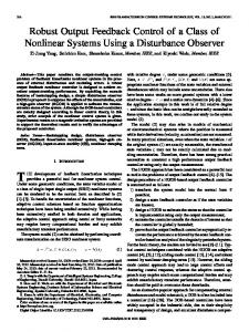
Simulations of the system in (39) under the adaptive control law (17) and (20) have been performed. The upper bounds on actuator actual spacing d M = d r − dl = 35 is assumed unknown. In order to demonstrate the performance improvement accomplished by our proposed method, the system under test given in (39) was used. The efficacy of the proposed method is proven by comparing its performance against the performance of a classic PD controller having equivalent gains. The complete parameters of the system under test and controller gains are listed in Table 1. The simulation results presented in Figure 2 and Figure 3, clearly show the tracking performance for x1 and x2 states along with their respective reference trajectory. Figure 4 and Figure 5 demonstrate the tracking error for the states x1 and x2 in blue in addition to the same tracking errors for the system under a PD controller in red. In both figures, the PD controller resulted in limit cycles where as the adaptive controller proved to be stable with no limit cycles and improved performance with a zero approaching tracking error. Figure 6 shows the control effort ud ( t ) and DZ ( ud ) . In Figure 7 the evolution of the βˆ which clearly demonstrates the boundedness of the adaptation. In Figure 8, the reference trajectory is changed to demonstrates a superior a step response performance when compared with PD controller. While the step error is approaching zero for the system under the proposed adaptive controller, a steady state error is persistent with the PD controller. Tracking Performance 5
Reference Signal r(t)
Radians
4
X_1
r(t) Refernce X(1)-State
3 2 1 0 -1
X1 state
-2 -3
0
0.5
1
1.5
2
2.5
Time (Seconds)
Figure 2. The tracking performance of x1 state of the system under the proposed robust controller.
16
3
N. J. Ahmad et al.
Tracking Performance 25
r(t) Refernce X(2)-State
20
Rad/S
15
X(2)
10 5 0 -5 -10 -15
0
0.5
1
1.5
2
Time (Seconds)
Figure 3. The tracking performance of x2 state of the system. Tracking Performance
Radians
4
PD Error X(1)-X(1)m error
3
Tracking Error
2
1
0
-1
-2
0
1
2
3
4
5
Time (Seconds)
Figure 4. The adaptively compensated tracking error x1 (blue) vs. the same tracking error of the system under a PD controller (red). Tracking Performance 8
PD Error X(2)-X(2)m error
6 4
Tracking Error
2 0 -2 -4 -6 -8 -10 -12 -14
0
1
2
3
4
5
Time (Seconds)
Figure 5. The adaptively compensated tracking error x2 (blue) vs. the same tracking error of the system under a PD controller (red).
17
N. J. Ahmad et al.
Control Signals 200
Control v(t) DZ(v) Output
150 100
N-m
50 0 -50 -100 -150 -200 0
0.5
1
1.5
2
Time (Seconds)
Figure 6. The control effort DZ ( ud ) in red vs. v = ud for the deadzone compensated system. Evolution of Adaptation 250
Adaptation Beta
200
150
100
50
0 0
1
2
3
4
5
Time (Seconds)
Figure 7. Evolution of the adaptation βˆ . Step Tracking Error 5
PD Adaptive
Unit Step Error Gain
4
3
2
1
0
-1
0
0.5
1.5
1
2
Time (Seconds)
Figure 8. Step tracking performance error for x1 for input r ( t ) = 1 .
18
2.5
3
N. J. Ahmad et al.
5. Conclusion
A robust adaptive controller is used to control a class of nonlinear systems with input deadzone nonlinearity at the input. The robust controller was shown to be superior in performance when compared to a more conventional control method such as a PD controller. The system under the proposed scheme has been shown to not only effectively stabilize a second order complex nonlinear system with disturbance, but also achieve asymptotic tracking. The advantage of the proposed method lies in the fact that no knowledge of the deadzone parameters needed and only an upper bound for the deadzone spacing is required. The adaptive deadzone inverse controller is smoothly differentiable and can easily be combined with any of the advanced control methodologies. The asymptotic stability of the closed-loop system has been proven by using Lyapunov arguments and simulation results confirmed the efficacy of the control methodology.
Funding This work is supported and funded by the Public Authority of Applied Education and Training, Research Project No. (TS-14-03) t, Research Title (Adaptive Control of Systems with Output Deadzone).
References [1]
Recker, D.A. and Kokotovic, P.V. (1993) Indirect Adaptive Nonlinear Control of Discrete-Time Systems Containing a Deadzone. Proceedings of the 32nd Conference on Decision and Control, 15-17 December 1993, San Antonio, 2647, 2653.
[2]
Toa, G. and Kokotovic, P. (1994) Adaptive Control of Plants with Unknown Dead-Zones. IEEE Transactions on Automatic Control, 39, 59-68. http://dx.doi.org/10.1109/9.273339
[3]
Tao, G. and Kokotovic, P. (1995) Discrete-Time Adaptive Control of Systems with Unknown Dead-Zones. International Journal of Control, 61, 1-17. http://dx.doi.org/10.1080/00207179508921889
[4]
Lewis, F.L., Tim, W.K., Wang, L.-Z. and Li, Z.X. (1999) Deadzone Compensation in Motion Control System Using Adaptive Fuzzy Logic Control. IEEE Transactions on Control Systems Technology, 7, 731-742. http://dx.doi.org/10.1109/87.799674
[5]
Selmic, R.R. and Lewis, F.L. (2000) Deadzone Compensation in Motion Control Systems Using Neural Networks. IEEE Transaction of Automatic Control, 45, 602-613.
[6]
Wang, X.-S., Su, C.-Y. and Hong, H. (2004) Robust Adaptive Control of a Class of Nonlinear Systems with Unknown Dead-Zone. Automatica, 40, 407-413.
[7]
Zhonghua, W., Bo, Y., Lin, C. and Shusheng, Z. (2006) Robust Adaptive Deadzone Compensation of DC Servo System. IEE Proc.-Control Theory Application, 153, 709-713.
[8]
Sedighi, H.M., Shirazi, K.H. and Zare, J. (2012) Novel Equivelent Function for Deadzone Nonlinearity: Applied to Analytical Solution of Beam Vibration Using He’s Parameter Expanding Method. Latin American Journal of Solids and Structures, 9, 1-10.
[9]
Ahmad, N.J., Alnaser, M.J. and Alsharhan, W.E. (2013) Asymptotic Tracking of Systems with Non-Symmetrical Input Deadzone Nonlinearity. International Journal of Automation and Power Engineering, 2, 287-292.
[10] Ahmad, N.J., Ebraheem, H., Alnaser, M. and Alostath, J. (2011) Adaptive Control of a DC Motor with Uncertain Deadzone Nonlinearity at the Input. Control and Decision Conference (CCDC), 4295-4299. [11] Sedighi, H.M., Shirazi, K.H. and Zare, J. (2012) Novel Equivelent Function for Deadzone Nonlinearit: Appled to Analytical Solution of Beam Vibration Using He’s Parameter Expanding Method. Latin American Journal of Solids and Structures, 9, 443-451. http://dx.doi.org/10.1590/S1679-78252012000400002 [12] Jain, S. and Khorrami, F. (1995) Robust Adaptive Control of a Class of Nonlinear Systems: State and Output Feedback. Proceeding of the 1995 American Control Conference, Seatle, 1580-1584. [13] Sankaranarayanan, S., Melkote, H. and Khorrami, F. (1999) Adaptive Variable Structure Control of a Class of Nonlinear Systems with Nonvanishing Perturbations via Backstepping. Proceedings of the American Control Conference, San Diego, 4491-4495. [14] Zhang, T.P. and Feng, C.B. (1997) Adaptive Fuzzy Sliding Mode Control for a Class of Nonlinear Systems. ACTA Automatica Sinica, 23, 361-369.
19