Robust Adaptive Minimum-Time Control of Piecewise Affine ... work of adaptive control [5], [19], [9]. .... xk which can be steered into Sk by some uk â U in one.
Joint 48th IEEE Conference on Decision and Control and 28th Chinese Control Conference Shanghai, P.R. China, December 16-18, 2009
WeC10.4
Robust Adaptive Minimum-Time Control of Piecewise Affine Systems ˇ Michal Kvasnica, Martin Herceg, L’uboˇs Cirka, and Miroslav Fikar Abstract— This paper illustrates how an adaptive model predictive controller for the class of hybrid systems affected by parametric uncertainties can be synthesized. Specifically, we investigate the case where the hybrid system is modeled as a Piecewise Affine (PWA) system where certain elements of the PWA state-update matrices are expressed as symbolic parameters with unknown, but bounded values. For such parametric uncertain PWA systems we show that the control law can be constructed in a way such that all system states are pushed towards a pre-defined target set in the minimal possible number of time steps for all possible realizations of the uncertainty. The robust minimum-time control problem is solved using parametric programming techniques which leads the control law in a form of a look-up table. We illustrate that if the values of the parameters (unknown at the time of the synthesis of the control law) are measured on-line, the resulting feedback policy guarantees timeoptimal convergence of the systems states towards a chosen terminal set.
I. INTRODUCTION PWA systems represent a powerful tool to describe the evolution of hybrid systems [21] and can be shown to be equivalent to many other hybrid system classes [12] such as mixed logical dynamical systems, linear complementary systems, and max-min-plus-scaling systems and thus form a very general class of linear hybrid systems. Moreover, PWA systems can be used to identify or approximate generic nonlinear systems via multiple linearizations at different operating points [21]. Although hybrid systems (and in particular PWA systems) are a special class of nonlinear systems, most of the nonlinear system and control theory does not apply because it usually requires certain smoothness assumptions. For the same reason we also cannot simply use linear control theory in some approximate manner to design controllers for PWA systems. Model predictive control of PWA systems has garnered increasing interest in the research community because it allows optimal control inputs for discrete-time PWA systems to be obtained by solving mixed-integer optimization problems on-line [3], [17], or as was shown in [1], [8], [14], [7], by solving off-line a number of multi-parametric programs. By multi-parametric programming, a linear (mpLP) or quadratic (mpQP) optimization problem is All authors are with the Institute of Information Engineering, Automation, and Mathematics, Faculty of Chemical and Food Technology, Slovak University of Technology in Bratislava, Slovakia {michal.kvasnica,martin.herceg,lubos.cirka,
miroslav.fikar}@stuba.sk
978-1-4244-3872-3/09/$25.00 ©2009 IEEE
solved off-line for a range of parameters. The associated solution (the explicit representation of the optimal control law) takes the form of a PWA state feedback law. In particular, the state-space is partitioned into polyhedral regions in which the optimal control law is given as an affine function of the state. In the on-line implementation of such controllers, input computation reduces to a simple set-membership test. Even though the benefits of this procedure in terms of cheap implementation are self evident, one major drawback of the parametric approach to MPC is the solution itself. Once calculated off-line, the solution is, so to say, “set in stone” and it can only be changed by repeating the off-line calculation. This might be necessary e.g. when the knowledge of plant model used to formulate the underlying optimization problem is updated. This is a frequent requirement in control of real plants, because the precise values of some (or all) model parameters are not known exactly and they often fluctuate in time. This issue is usually tackled by adopting the framework of adaptive control [5], [19], [9]. In this policy, the values of unknown parameters are measured, estimated or identified on-line and the process model is updated accordingly. For the newly obtained model, a new control problem is formulated and solved to take the updated knowledge into account. This repetitive parameter estimation and control optimization is particularly suitable in classical on-line MPC. However, it goes against the spirit of parametric solutions to MPC problems, where the solution is calculated just once for a fixed process model. To circumvent this problem and to keep the advantages of the off-line MPC approach, [2] and [4] proposed, for linear and LPV systems, respectively, a method of solving a max-min control problem parametrically while providing (i) robust feasibility and (ii) optimal performance in terms of minimizing a given objective function over a fixed prediction horizon. In this paper we first extend these ideas to PWA systems, whose dynamics is affected by a some timevarying parameters. Parameter values are not known at the time of the synthesis of the control law, but will become available when the controller is evaluated online. The goal is to synthesize a control policy which drives all system states towards a given terminal set in the least possible number of time steps, i.e. in a minimum time fashion with respect to the system dynamics and constraints on states and control inputs. We illustrate how this problem can be solved off-line to
2454
WeC10.4 obtain the feedback law in a form of a look-up table, hence mitigating the on-line implementation effort. As will be shown later, this boils down to a non-convex problem. Therefore, in this article we also provide a new methodology of synthesizing feedback laws under the circumstances that the terminal sets are non-convex unions of convex polytopes. Once the closed-form representation of the control law is obtained off-line, robust feasibility and guaranteed convergence towards a chosen terminal set for any variation of the unknown system parameters within a given range is provided. Moreover, since the influence of the parameters is consider in the optimization objective, on-line measurements of these parameters can be used to update the control policy. Hence the proposed strategy acts as a robust minimumtime adaptive controller, where the control inputs are time-optimal for all values of the parametric uncertainty. Therefore, the updated knowledge of the process model can be taken into account by the controller at each time step. II. Problem Statement In this work we consider discrete-time PWA systems of the following form xk+1 = fPWA (xk , λk , uk ) = Ad (λk )xk + Bd uk + fd
if xk ∈ Dd ,
(1)
where xk ∈ Rnx is the system state, uk ∈ Rnu is the manipulated input, k ≥ 0 denotes the sampling instant, and Ad (λk ), Bd , fd are matrices of appropriate dimensions. Variable d ∈ [1, . . . , nD ] denotes the mode of the PWA system, with nD being the total number of modes. The system states and inputs are assumed to be bounded by, respectively, xk ∈ X ⊂ Rnx and uk ∈ U ⊂ Rnu where X and U are nonempty convex and compact sets. We assume that the system matrices Ad (λk ) depend on an unknown, but bounded parameter vector λk ∈ Λ. Furthermore we assume that Λ is a convex and compact set and that the unknown parameters λk enter Ad (λk ) in a linear fashion Ad (λk ) =
nλ X
λk,j Aji ,
(2)
j=1
P with j λk,j = 1 and 0 ≤ λk,j ≤ 1 for j ∈ [1, . . . , nλ ] and the total of nλ vertices A1d , . . . , And λ being given. If the whole state space domain is denoted SnD by D, then the overall PWA model is built by d=1 Dd regions, whereas one local model is valid in each region. Formally Dd is a nonempty compact set, defined in the state space, and it is given by a set of linear inequalities of the form � Dd = xk | Ddx xk ≤ Dd0 (3)
Problem 2.1: For the PWA system (1), find a feedback policy of the form u = g(x, λ),
(4)
which takes into account measurements (or estimates) of the current state x and measurements (or estimates) of the parameter vector λ, and drives all system states into Tset in the least possible number of steps for all possible values of the parameter vector λ ∈ Λ while respecting input and state constraints. Problem 2.1 is commonly referred to as a minimumtime problem [13], [6], [18], [11], [20]. As shown e.g. in [11], if the PWA system (1) is not subject to the parametric uncertainty (2) (i.e. for nλ = 1), the minimumtime problem can be solved using dynamic programming (DP), i.e. by solving 1-step problems backwards in time. At each iteration of the DP procedure the feedback law u∗k (xk ) minimizing a given performance measure J(xk , uk ) is obtained, explicitly, by solving a multi-parametric program. The feedback is such that for all xk ∈ Sk the one-step predicate xk+1 is pushed “one step closer” to the given initial terminal set, i.e. fPWA (xk , u∗k (xk )) ∈ Sk−1 . There are two reasons why these standard approaches cannot be directly applied to solve Problem 2.1: (i) λk and xk are optimized parameters, thus the PWA dynamics is nonlinear due to their bi-product in (1), and (ii) the resulting variations of the parameter vector λk in the set Λ. This is equivalent to solution of a non-convex minimum-time problem for a PWA system with statedependent disturbances. Both issues make Problem 2.1 far from trivial. III. Synthesis of an Adaptive Minimum-Time Controller In this section we show how to solve Problem 2.1 parametrically, i.e. we obtain an explicit representation of the function g(xk , λk ) for all admissible values of xk and λk . Solving the problem faces following challenges: C1: Deal with the fact that the PWA dynamics (1) is bi-linear in xk and λk . C2: Give a procedure for computing robust one-step reachable sets for PWA systems with parametric uncertainties, i.e. find P re(Sk ) ={xk | ∃uk ∈ U, s.t.
(5)
fPWA (xk , λk , uk ) ∈ Sk , ∀λk ∈ Λ}. C3: Find an explicit representation of the feedback law (4) in such a way that measurements of λk are taken into account when minimizing
where Ddx and Dd0 are matrices of suitable dimensions specifying the borders of the d-th region Dd . For the PWA system (1) this paper shows how to solve the following problem:
2455
J(xk , λk , uk ) = kQx xk+1 k1 + kQu uk k1 ,
(6)
allowing (4) to adapt the control action to the currently available value of λk . Here, xk+1 = fPWA (xk , λk , uk ), cf. (1), k·k1 denotes a standard 1norm of a vector and Qx , Qu are weighting matrices of suitable dimensions.
WeC10.4 Challenge C1 can be attacked by observing that (1) is linear in the joint product Ad (λk )xk for a fixed mode d. Following the ideas of [2] and [4] we propose to introduce an auxiliary information variable zk to convert the bilinear PWA form into a linear one: xk+1 = fPWA (zk , uk ) = zk + Bd uk + fd .
the set Zk,i,d will be a convex polytope and its projection therefore also will be a polytope [22]. Hence P re(Sk ) will be a collection of convex polytopes. Optimal control action uk minimizing the cost (6) in C3 can be found by solving the following horizon-1 nonconvex optimization problem: min
(7)
uk
s.t.
The information variable zk given by zk (xk , λk , d) = Ad (λk )xk
(8)
captures both the knowledge of the mode d active at the time instance k as well as the state contribution Ad (λk )xk for the actually measured value of the parameter vector λk . Remark 3.1: Important to notice is that the augmented PWA system (7) is equivalent to the original form of (1), for one time step, if the state xk , the value of the parameter vector λk , and the active mode d are known at time k such that zk (·) can be evaluated per (8). This is not a restrictive requirement, but a direct consequence of the adaptive control strategy. As for any other statefeedback policy, the current state xk has to be measured (or estimated), and the values of the parameters λk will either be directly measured, or obtained e.g. using recursive identification techniques at each discrete time instance k. For a given xk , the active mode d is uniquely determined by (3). illustrate solution to C2, we denote by Sk = SnTo S S i=1 k,i the (possibly non-convex) union of nS convex polytopes Sk,i . Then we get the following result. Lemma 3.2: For the PWA system (1) the set of states xk which can be steered into Sk by some uk ∈ U in one time step for all possible values of λk ∈ Λ is given as a (possibly non-convex) union of convex polytopes P re(Sk ) =
nS n D [ [
projx (Zk,i,d )
(9)
i=1 d=1
with Zk,i,d =
n
[ uxkk ] uk ∈ U, xk ∈ Dd ,
Ajd xk + Bd uk + fd ∈ Sk,i , o ∀j ∈ [1, . . . , nλ ]
(10)
where projx (Zk,i,d ) denotes the orthogonal projection of the set Zk,i,d onto x. Proof: Notice that Ajd xk + Bd uk + fd ∈ Sk,i ∀j ∈ [1, . . . , nλ ] can be written in an expanded form as A1d x + Bd u + fd And λ x + Bd u + fd
J(xk , λk , uk )
(11a)
uk ∈ U
(11b)
xk ∈ D
(11c)
xk+1 ∈ Sk xk+1 = fPWA (zk (xk , λx , d), uk )
(11d) (11e)
Remark 3.3: By Lemma 3.2 and Remark 3.1 the set of xk for which (11b)–(11e) is feasible is given by P re(Sk ). By considering the augmented PWA model (7) in (11e), the influence of the measured parameters λk on J(·) is taken into account when optimizing for the values of uk . Non-convexity of (11) stems from two reasons. First, the PWA state-update equation in (11e) is nonlinear due to the presence of “IF-THEN” rules in (1). Secondly, Sk in (11d) is, in general, givenSas a non-convex union of convex polytopes, i.e. Sk = i Sk,i . However, if the performance measure J(·) in (11) is as in (6), and for a fixed d and fixed i, problem (11) boils down to a convex linear programming (LP) problem in variables uk and zk . If zk is considered as a parameter, feedback law (4) can be obtained, for all admissible values of zk , by solving (11) as an mpLP: Theorem 3.4 ([7]): The optimal solution to (11) for all admissible values of zk (·) is, for a fixed i and d, a piecewise affine state-feedback control law and a PWA representation of the optimal cost in the form r u∗k,i,d (zk (·)) = Fk,i,d zk (·) + Grk,i,d
if zk (·) ∈ Rrk,i,d , (12) ∗ r Jk,i,d (zk (·)) = Lrk,i,d zk (·) + Mk,i,d if zk (·) ∈ Rrk,i,d , n o (13) r r r where Rk,i,d = zk (·) | Hk,i,d zk (·) ≤ Kk,i,d , r = 1, . . . , Rk,i,d is a set of polyhedral S (or polytopic) regions. Moreover, the set Pk,i,d = r Rrk,i,d of all zk for which (11) is feasible at time k is a convex set. Theorem 3.5 ([7]): If (11) is solved consecutively ∀i ∈ [1, . . . , nS ], ∀d ∈ [1, . . . , nD ], an explicit representation of the optimal feedback law u∗k (zk (·)) given by ∗ u∗k (zk (·)) = arg min Jk,i,d (zk (·)) i,d
is also a PWA function of zk (·), i.e. u∗k (zk (·)) = Fkr zk (·) + Grk
∈ Sk,i , .. . ∈ Sk,i
which enforces that fPWA (xk , λk , uk ) ∈ Sk,i holds for all λk ∈ Λ. As Sk,i , U, and Dd are assumed to be convex,
(14)
if zk (·) ∈ Rrk
(15)
with Rrk = {zk (·) | Hkr zk (·) ≤ Kkr }. Theorem 3.5 suggests that an explicit representation of u∗k (zk (·)) solving C3 can be found by solving nS · nD mpLP’s and subsequently by taking the minimum among ∗ the same number of PWA optimal costs Jk,i,d .
2456
WeC10.4 Remark 3.6: Multi-parametric linear programs can be solved e.g. using the freely available Multi-Parametric Toolbox (MPT) [15], which also provides calculation of the minimum among several PWA cost functions in (14). We can now state the main result of the paper, which is a procedure for designing an adaptive controller which will utilize the measurements of the parameter vector λ to update the control policy. The problem is solved parametrically, which means that the whole control synthesis can be performed off-line. On-line implementation of such a controller will reduce to a simple set-membership test. The computation of the controller is carried out using Algorithm 1. Algorithm 1 The minimum-time adaptive algorithm INPUT: PWA system (1), weighting matrices Qx , Qu of (6), initial terminal set Tset . OUTPUT: Integer k ∗ , sets Sk , PWA feedback laws u∗k (zk (·)). 1: k ← 0, Sk ← Tset . 2: repeat 3: Obtain u∗k (zk (·)) in the form of (15) by solving (11) as nS · nD mpLPs. 4: Compute P re(Sk ) by Lemma 3.2. 5: Sk+1 ← P re(Sk ). 6: k ← k + 1. 7: until Sk+1 6= Sk 8: k ∗ ← k. Theorem 3.7: The feedback laws u∗k (zk (·)), k = [0, . . . , k ∗ ] calculated by Algorithm 1 are such that the PWA system (1) can be robustly pushed to Tset ∀λ ∈ Λ in, at most, k ∗ steps for any x ∈ P re(Sk∗ ). Moreover, measurements of λ are taken into account by u∗k (zk (·)) to further optimize for performance. Proof: At iteration k for any x0 ∈ Sk the feedback law obtained in Step 3 is such that the one-step predicate x1 = fPWA (x0 , λ0 , u∗k (x0 )) is pushed into Sk−1 in one time step ∀λ0 ∈ Λ by construction (cf. (11d)). Robustness is ensured by taking Sk = P re(Sk−1 ) computed by Lemma 3.2. The iterative nature of the algorithm guarantees that for any x1 ∈ Sk−1 we have x2 = fPWA (x1 , λ1 , u∗k−1 (x1 )) ∈ Sk−2 , ∀λ1 ∈ Λ again by Step 3. By consecutively applying the feedback laws u∗k−2 (x2 ), u∗k−3 (x3 ), . . . , u∗0 (xk ) we therefore get xk+1 ∈ S0 (note that S0 = Tset by Step 1). Hence all states of the PWA system (1) are pushed towards Tset in, at most, k ∗ steps due to the stopping criterion in Step 7. By employing (8) in the performance objective (11a) we have that the knowledge of λk is taken into account when optimizing for u∗k at each iteration. Remark 3.8: To attain stability, Tset along with a feedback law u∗set active for all x ∈ Tset must be chosen such that the terminal set is invariant, i.e. xk ∈ Tset ⇒ xk+j ∈ Tset , ∀j > 0. Finding such terminal set along with the terminal controller is however, outside of the scope of this work.
Remark 3.9: The minimal number of steps k ∗ in which all system states can be steered into Tset is automatically identified in Step 8 upon convergence of Algorithm 1. This quantity is governed by feasibility of problem (11). Remark 3.10: It should be noted that, at each iteration k, multiple control actions uk might exist such that (11b)–(11e) hold. In such a case the performance index (11a) is used to select a unique solution in (14). Remark 3.11: Complexity of the look-up table can be further reduced at each iteration k of Algorithm 1 in Step 3 by merging together regions whose union is convex and they share the same control law, see e.g. [10]. Efficient algorithms to perform such a reduction are included in [15]. In general, for PWA systems the sets Sk would overlap, i.e. there are multiple k’s for which x ∈ Sk . Therefore, the consecutive application of different feedback laws at different steps must be performed such that a proper value of the index k is chosen for each x. Such a procedure is captured by Algorithm 2, which shows how the minimum-time adaptive controller is implemented online. Algorithm 2 On-line implementation INPUT: Measurements of the current state x and the parameter vector λ, sets P re(Sk ), feedback laws u∗k (zk (·)), ∀k = [0, . . . , k ∗ ]. OUTPUT: Optimal value of the control action u∗ . 1: Find the minimal value of the index j for which x ∈ P re(Sj ). 2: Calculate z(·) from (8) by utilizing the knowledge of λ and x. 3: From the j-th feedback law of the form of (15) find the region index r for which z(·) ∈ Rrj . 4: Calculate optimal control action by u∗ = Fjr z(·)+Grj .
Theorem 3.12: The minimum-time adaptive controller calculated by Algorithm 1 and applied to a PWA system (1) in a receding horizon control fashion according to Algorithm 2 guarantees that all states are pushed towards Tset in the minimal possible number steps. Proof: Assume the initial state x is contained in the set P re(Sj ) from which it takes j steps to reach Tset according to Theorem 3.7. The control law identified by Algorithm 2 will drive the states into the set P re(Sj−1 ) in one time step. Therefore, the states will enter Tset in j steps when Algorithm 2 called repeatedly at each sampling instance. Therefore, the control law calculated by Algorithm 1 acts as an adaptive controller when implemented on-line and the measurements of λk can be used to update the process model. The controller is calculated off-line in a form of a look-up table, reducing the on-line implementation effort to a sequence of simple set-membership tests.
2457
WeC10.4 6
x0 = [0, − 5]T . Profile of the uncertainty, together with the optimal control moves and the closed-loop evolution of system states are depicted, respectively, in Figures 2, 4, and 3. As can be seen from the plots, the minimum-time controllers adapts itself to the current measurements of the parameter w and drives all system states towards the terminal set despite quite substantial variations of the value of the uncertainty.
4
z2
2
0
ï2
1.05 hk 1
ï4
0.95
0
z1
5 0.9
hk
ï6 ï5
Fig. 1. Regions Rk of the PWA feedback laws u∗k (z(·)). By the same colors are depicted regions from the same iteration k. More reddish regions correspond to lower values of k.
0.85 0.8 0.75
IV. Example
0.7
In this section we illustrate the application of Algorithm 1 to a modified version of the periodic PWA system of [3]. The dynamics of such a system is given by ( (1) A1 xk + Buk IF xk < 0 xk+1 = (16) (1) A2 xk + Buk IF xk ≥ 0,
0.65 0
10
15
20
k
Fig. 2. w.
Time-varying fluctuations of the value of the uncertainty
4
(1)
where xk denotes the first coordinate of the state vector xk . State-update matrices for each of the two modes of the PWA system are given by � � � � 0 cos(αi ) − sin(αi ) , B= Ai = w , (17) 1 sin(αi ) cos(αi )
x1 3
x2
2
Tset
1 0
xk
with α1 = −π/3 and α2 = π/3, respectively. We assume that the value of the parameter w is unknown at the time of the synthesis of the control law, but it is bounded by 0.7 ≤ w ≤ 1. The vertices A1i , A2i in (2) can be obtained by evaluating Ai from (17) for boundary values of this interval. We have then implemented Algorithm 1 by employing the Multi-Parametric Toolbox [15] to calculate projections in Lemma 3.2 and to solve (11) parametrically. YALMIP [16] was used to formulate (11) in a userfriendly fashion. Problem 2.1 was then solved with X = {x | − 5 ≤ x ≤ 5}, U = {u | − 1 ≤ u ≤ 1}, and Tset = {x | − 0.5 ≤ x ≤ 0.5}. Algorithm 1 has converged at iteration 8 after 235 seconds, generating 5 PWA feedback laws of the form (14), which are parameterized in the information variable z(x, λ, d). Regions over which these control laws are defined are depicted in Figure 1. In the spirit of adaptive control we have investigated the behavior of the proposed minimum-time scheme when the value of the uncertainty w fluctuates over time. To do that we have generated a random sequence of wk satisfying 0.7 ≤ wk ≤ 1 and subsequently performed closed-loop simulations starting from the initial state
5
ï1 ï2 ï3 ï4 ï5 0
5
10
15
20
k
Fig. 3.
Closed-loop profiles of x.
V. Conclusions The paper showed how to synthesize robust adaptive minimum-time controllers for the class of PWA systems affected by parametric uncertainties. The control policy is synthesized in such a way that all system states are pushed towards a prescribed terminal set in the least possible number of time steps for all admissible values of the uncertainty. The controller is calculated using parametric optimization which results in a feedback law in a form of a look-up table, parameterized in the influence of the uncertain parameters. On-line measurements of
2458
WeC10.4 u*(z) umin / umax
1 0.8 0.6 0.4
u*k(z)
0.2 0 ï0.2 ï0.4 ï0.6 ï0.8 ï1 0
5
10
15
20
k
Fig. 4.
Closed-loop profiles of u∗ .
the uncertainty can thus be used to further optimize for performance when the controller is implemented in the receding horizon fashion. VI. ACKNOWLEDGMENTS The authors are pleased to acknowledge the financial support of the Scientific Grant Agency of the Slovak Republic under the grants 1/0071/09 and 1/4055/07. This work was supported by the Slovak Research and Development Agency under the contracts No. VV-002907 and No. LPP-0092-07. References [1] M. Baoti´ c, F. J. Christophersen, and M. Morari. A new Algorithm for Constrained Finite Time Optimal Control of Hybrid Systems with a Linear Performance Index. In European Control Conference, Cambridge, UK, September 2003. [2] M. Baric, Sasa V. Rakovic, Th. Besselmann, and M. Morari. Max-Min Optimal Control of Constrained Discrete-Time Systems. In IFAC World Congress, July 2008. [3] A. Bemporad and M. Morari. Control of systems integrating logic, dynamics, and constraints. Automatica, 35(3):407–427, March 1999. [4] Th. Besselmann, J. L¨ ofberg, and M. Morari. Explicit MPC for systems with linear parameter-varying state transition matrix. In International Federation of Automatic Control World Congress, July 2008. [5] R. R. Bitmead, M. Gevers, and V. Wertz. Adaptive Optimal Control: The Thinking Man’s GPC. International Series in Systems and Control Engineering. Prentice Hall, 1990. [6] F. Blanchini. Minimum-Time Control for Uncertain DiscreteTime Linear Systems. In Proc. of the Conf. on Decision & Control, pages 2629–2634, Tucson, AZ, USA, December 1992. [7] F. Borrelli. Constrained Optimal Control of Linear and Hybrid Systems. In Lecture Notes in Control and Information Sciences, volume 290. Springer, 2003. [8] F. Borrelli, M. Baoti´ c, A. Bemporad, and M. Morari. An efficient algorithm for computing the state feedback optimal control law for discrete time hybrid systems. In Proc. of the American Control Conference, Denver, Colorado, USA, June 2003. [9] P. Dost´ al, M. Bakoˇsov´ a, and V. Bob´ al. An approach to adaptive control of a cstr. Chemical Papers, 58(3):184–190, 2004. [10] T. Geyer, F. D. Torrisi, and M. Morari. Optimal Complexity Reduction of Piecewise Affine Models Based on Hyperplane Arrangements. In Proc. on the American Control Conference, pages 1190–1195, Boston, Massachusetts, USA, June 2004.
[11] P. Grieder, M. Kvasnica, M. Baotic, and M. Morari. Stabilizing low complexity feedback control of constrained piecewise affine systems. Automatica, 41, issue 10:1683–1694, Oct. 2005. [12] W. P. M. Heemels, B. De Schutter, and A. Bemporad. Equivalence of hybrid dynamical models. Automatica, 37(7):1085– 1091, 2001. [13] S. S. Keerthi and E. G. Gilbert. Computation of MinimumTime Feedback Control Laws for Discrete-Time Systems with State-Control Constraints. IEEE Trans. on Automatic Control, AC-32:432–435, May 1987. [14] E. C. Kerrigan and D. Q. Mayne. Optimal control of constrained, piecewise affine systems with bounded disturbances. In Proc. 41st IEEE Conference on Decision and Control, Las Vegas, Nevada, USA, December 2002. [15] M. Kvasnica, P. Grieder, M. Baotic, and M. Morari. MultiParametric Toolbox (MPT). In Hybrid Systems: Computation and Control, pages 448–462, March 2004. Available from http: //control.ee.ethz.ch/˜mpt. [16] J. L¨ ofberg. YALMIP : A Toolbox for Modeling and Optimization in MATLAB. In Proc. of the CACSD Conference, Taipei, Taiwan, 2004. Available from http://control.ee.ethz. ch/˜joloef/yalmip.php. [17] D. Q. Mayne and S. Rakovi´ c. Model predictive control of constrained piecewise affine discrete–time systems. Int. J. of Robust and Nonlinear Control, 13(3):261–279, April 2003. [18] D. Q. Mayne and W. R. Schroeder. Robust time-optimal control of constrained linear Systems. Automatica, 33(12):2103– 2118, December 1997. [19] E. Mosca. Optimal, Predictive, and Adaptive Control. Prentice Hall, Englewood Cliffs, New York, 1995. [20] S.V. Rakovi´ c, P. Grieder, M. Kvasnica, D.Q. Mayne, and M. Morari. Computation of Invariant Sets for Piecewise Affine Discrete Time Systems subject to Bounded Disturbances. In Proceeding of the 43rd IEEE Conference on Decision and Control, pages 1418–1423, Atlantis, Paradise Island, Bahamas, December 2004. [21] E. D. Sontag. Nonlinear regulation: The piecewise linear approach. IEEE Trans. on Automatic Control, 26(2):346–358, April 1981. [22] G. M. Ziegler. Lectures on Polytopes. Graduate Texts in Mathematics. Springer-Verlag, 1995.
2459