Addison-Wesley Inc. 1980. [26]Cohen, E., âSome Mathematical Tools for a Modeler's. Workbench,â IEEE Comp. Graph. and App., 3(7), Oct. 1983. [27] Voorhies ...
Robust and Efficient Cartesian Mesh Generation for Component-Based Geometry M.J. Aftosmis* U.S. Air Force Wright Laboratory / NASA Ames Moffett Field, CA 94035 † M.J. Berger J.E. Melton‡ Courant Institute NASA Ames Research Center New York, NY 10012 Moffett Field, CA 94035
Abstract This work documents a new method for rapid and robust Cartesian mesh generation for componentbased geometry. The new algorithm adopts a novel strategy which first intersects the components to extract the wetted surface before proceeding with volume mesh generation in a second phase. The intersection scheme is based on a robust geometry engine that uses adaptive precision arithmetic and which automatically and consistently handles geometric degeneracies with an algorithmic tie-breaking routine. The intersection procedure has worse case computational complexity of O(N logN) and is demonstrated on test cases with up to 121 overlapping and intersecting components including a variety of geometric degeneracies. The volume mesh generation takes the intersected surface triangulation as input and generates the mesh through cell division of an initially uniform coarse grid. In refining hexagonal cells to resolve the geometry, the new approach preserves the ability to directionally divide cells which are well-aligned with local geometry. The mesh generation scheme has linear asymptotic complexity with memory requirements that total approximately 14 words/cell. The mesh generation speed is approximately 106cells/minute on a 195Mhz RISC R10000 workstation.
I. Introduction The past several years have seen a large resurgence of interest in adaptive Cartesian mesh algorithms for application to problems involving complex geometries. Refs. [1-12], among others, have proposed flow solvers and mesh generation schemes intended for use with arbitrary geometries. Since generating suitable Cartesian meshes is relatively quick, and the process can be fully automated, much of the on-going research focuses on quick extraction of CFD-ready geometry from the CAD databases to provide easy access to accurate solutions of Euler equations within the design cycle. Viewing configurations on a component basis has several conceptual advantages over treatments which work with a single complete configuration. The most obvious of these is that components can be translated/ *. Aerospace Engineer, Senior Member AIAA †. Prof. Dept. of Comp. Sci., Member AIAA ‡. Aerospace Engineer, Senior Member AIAA This paper is declared a work of the U.S. Government and is not subject to copyright protection in the United States.
rotated with respect to one another without requiring user intervention or a time consuming return to CAD in order to extract new intersection information and a new CFD-ready description of the wetted surface. Many approaches begin with a surface triangulation already constrained to the intersection curves of the components[9]. By starting upstream in the process, the component-based approach requires only that each piece of the geometry be described as a single closed entity. Thus, relative motion of parts may be pre-programmed or even computed as a result of a design analysis. The approach offers obvious advantages for automation through external, macroscopic control. This flexibility comes at the expense of added complexity within the grid generation process. Since components may overlap, the possibility exists that a Cartesian cell-surface intersection detected during mesh generation may be entirely internal to the configuration, and thus all such intersections must be classified as “exposed” (retain) or “internal” (reject). Even if the vast majority of such intersections are actually part of the wetted surface, all intersections have the possibility of being internal, and therefore must be tested. An analysis of the mesh generation procedure documented in Refs.[1] and [13] revealed that up to 60% of the computation was dedicated to the resolution of this issue. Although several approaches toward streamlining the process exist, the most attractive appears to be one which avoids the issue of intersection classification altogether. By first intersecting all components together, one can extract precisely the wetted surface so that all subsequent Cartesian cell intersections are guaranteed to be “exposed” and therefore retained. The remaining mesh generation problem may then be treated as if it were a single component problem. While conceptually straightforward, efficient implementation of such an intersection algorithm is delicate. Each component is assumed to be described by a surface triangulation and the solution involves a sequence of problems in computational geometry. The
algorithm requires intersecting a number of non-convex polyhedra with arbitrary genus. This makes convex polyhedra intersection algorithms inappropriate. Each intersected triangle must be broken up into smaller ones, which is a problem in constrained triangulation. Finally, the deletion of the interior triangles requires inside/outside determination and neighbor painting. Since intersecting triangles from different components must be considered to be in general position, the specters of robustness and finite precision mathematics must be considered as well. Section II presents a robust algorithm for computing these intersections and extracting the wetted surface on realistically complex examples. This algorithm is quite general and has numerous applications outside the specific field of CFD. Section III presents the volume mesh generation algorithm with particular attention to the efficiency of data structures and the speed of intersection tests. The approach preserves the ability to directionally refine mesh cells. This feature comes in response to earlier work which concluded that isotropic cell division may lead to excessive numbers of Cartesian cells in three dimensions[13]. This work suggested that lower dimensional features may frequently be resolved by directional division of Cartesian cells.
II. Component Intersection The problem of intersecting the various components of a given configuration and extracting the wetted surface may be viewed as a series of smaller problems not uncommon in computational geometry. This section briefly discusses some of the key aspects involved in the process. Focus centers on the topics of proximity searching, primitive geometric operations, exact arithmetic and algorithms for breaking geometric degeneracies.
A. Proximity Queries Without special care, the intersection algorithm can result in implementations which have an asymptotic complexity of O(N2). The primary culprit here is the repetition of geometric searches to determine a list of candidate triangles on all components which may intersect with a given triangle on the polyhedron under consideration. A number of data structures have been proposed to speed up this process, and one particularly suitable method is the Alternating Digital Tree (ADT) algorithm developed in Ref.[14]. Inserting the triangles into an ADT makes it possible to identify the list of candidate triangles in O(logN) operations. As a result, intersections need only be checked against candidate
triangles from the list of spanning triangles returned from the tree. The basic algorithm outlined here follows from [14] and is implemented using the balanced tree approach detailed in Ref. [13]. The ADT is a hyperspace search technique which converts the problem of searching for finite sized objects in d dimensions to the simpler one of partitioning a space with 2d dimensions. Since searches are not conducted in physical space, objects which are physically close together are not necessarily close in the search space. This fact can hamper the tree’s performance in some instances[15]. In an effort to improve lookup times, we therefore first apply a component bounding-box filter on the triangles before inserting them into the tree. Since they cannot possibly participate in an intersection, triangles which are not contained by the bounding box of a component other than their own are not inserted into the tree. This filtering not only reduces the tree size but also improves the probability of encountering an intersection candidate within the tree, since the structure is not crowded with irrelevant geometry.
B. Intersection of Generally Positioned Triangles in R3 With the task of intersecting a particular triangle reduced to an intersection test between that triangle and those on the list of candidates provided by the ADT, the intersection problem is re-cast as a series of tri-tri intersection computations. Figure 1 shows a view of two intersecting triangles as a model for discussion. Each intersecting tri-tri pair will contribute one segment to the final polyhedra that will comprise the wetted surface of the configuration. The assumption of data in general (as opposed to arbitrary) position implies that the intersection is always nondegenerate. Triangles may not share vertices, and edges of tri-tri pairs do not intersect exactly. Thus, all intersections will be proper. This restriction will be lifted in later sections with the introduction of an automatic tie-breaking algorithm.
a 0
1 b 2
c
Figure 1: An intersecting pair of generally positioned triangles in three dimensions.
Several approaches exist to compute such intersections but a particularly attractive technique comes in the form of a Boolean test. This predicate can be performed robustly and quickly using only multiplication
-2-
and addition, thus avoiding the inaccuracy and robustness pitfalls associated with division using fixed width representations of floating point numbers. It is useful to present a rather comprehensive treatment of this intersection primitive because subsequent sections on robustness will return to these relations. For two triangles to properly intersect in three dimensional space, the following conditions must exist: 1. Two edges of one triangle must cross the plane of the other. 2. If condition (1) exists, there must be a total of two edges (of the six available) which pierce within the boundaries of the triangles.
One approach to checking these conditions is to directly compute the pierce points of the edges of one triangle in the plane of the other. Pierce locations from one triangle’s edges may then be tested for containment within the boundary of the other triangle. This approach, while conceptually simple, is error prone when implemented using finite precision mathematics. In addition to demanding special effort to trap out zeros, the floating point division required by this approach may result in numbers not exactly representable by finite width words. This results in a loss of control over precision and may cause serious problems with robustness. An alternative to this slope-pierce test is to consider a Boolean check based on computation of a triple product without division. A series of such logical checks have the attractive property that they permit one to establish the existence and connectivity of the segments without relying on the problematic computation of the pierce locations. The final step of computing the locations of these points may then be relegated to post-processing where they may be grouped together and, since the connectivity is already established, floating point errors will not have fatal consequences. The Boolean primitive for the 3D intersection of an edge and a triangle is based on the concept of the signed volume of a tetrahedron in R3. This signed volume is based on the well established relationship for the computation of the volume of a simplex, T, in d dimensions in determinate form (see for ex. [16]). The signed volume V(T) of the simplex T with vertices ( v 0, v 1, v 2, …, v d ) in d dimensions is: v0
0
d!V ( T v v v …v ) = det … 0 1 3 d v
d0
v0 … v0 1 1 d–1 … … … … v …v 1 d1 dd – 1
(1)
a0 a1 a2 1
6V ( T abcd ) =
(2)
= b0 – d0 b1 – d1 b2 – d2
c0 c1 c2 1
c0 – d0 c1 – d1 c2 – d2
d0 d1 d2 1
This volume serves as the fundamental building block of the geometry routines. It is positive when (a,b,c) forms a counterclockwise circuit when viewed from an observation point located on the side of the plane defined by (a,b,c) which is opposite from d. Positive and negative volumes define the two states of the Boolean test while zero indicates that the four vertices are exactly coplanar. If the vertices are indeed coplanar, then the situation constitutes a “tie” which will be resolved with a general tie-breaking algorithm presented shortly. In applying this logical test to edge ab and triangle (0,1,2) in fig. 1, ab crosses the plane if and only if (iff) the signed volumes T012a and T012b have opposite signs. Figure 2 presents a graphical look at the application of this test. a
a 1
a
1
1
0
0
0
P
P
2
2
b
2
b
Vol(T0,1,2,a ) < 0
Vol(T0,1,2,b ) > 0
b
Figure 2: Boolean test to check if edge ab crosses the plane defined by triangle (0,1,2) through computation of two signed volumes.
With a and b established on opposite sides of the plane (0,1,2), all that remains is to determine if ab pierces within the boundary of the triangle. This will be the case only if the three tetrahedra formed by connecting the end points of ab with the three vertices of the triangle (0,1,2) (taken two at a time) all have the same sign, that is: [ V ( T a12b ) < 0 ∧ V ( T a01b ) < 0 ∧ V ( T a20b ) < 0 ] or (3) [ V ( T a12b ) > 0 ∧ V ( T a01b ) > 0 ∧ V ( T a20b ) > 0 ] Figure 3 illustrates this test for the case where the three volumes are all positive. a a a 0 0 1 1 0 1 p 2 Ta,1,2,b
p
p 2
b
where vkj denotes the jth coordinate of the kth vertex with j, k ∈ { 0, 1, 2, …, d } . In 3 dimensions, eq. {2} gives six times the signed volume of the tetrahedron Tabcd.
a0 – d0 a1 – d1 a2 – d2
b0 b1 b2 1
2 b
Ta,0,1,b
b
Ta,2,0,b
Figure 3: Boolean test for pierce of a line segment ab within the boundary of a triangle (0,1,2).
After determining the existence of all the segments which result from intersections between tri-tri pairs and connecting a linked list of all such segments to the
-3-
triangles that intersect to produce them, all that remains is to actually compute the locations of the pierce points. This is accomplished by using a parametric representation of each intersected triangle and the edge which pierces it. The technique is a straightforward three dimensional generalization of the 2D method presented in reference [16].
are enforced using a simple recursive edge swapping routine.
d a b
C. Retriangulation of Intersected Triangles The final result of the intersection step is a list of segments linked to each intersected triangle. These segments divide the intersected triangles into polygonal regions which are either completely inside or outside of the body. In order to remove the portions of these triangles which are inside, we triangulate these polygonal regions within each intersected triangle and then reject the triangles which lie inside the body. Figure 4 shows a typical intersected triangle divided into two polygonal regions with the segments resulting from the intersection calculation highlighted. In the sketch, the two polygonal regions formed by the triangle’s boundary and the segments from the intersection have been decomposed into sets of triangles. Since the segments may cut the triangle arbitrarily, a pre-disposition for creating triangles with arbitrarily small angles exists. In an effort to keep the triangulations as wel behaved as possible, we employ a two dimensional Delaunay algorithm within each original intersected triangle. Using the intersection segments as constraints, the algorithm runs within each intersected triangle producing new triangles which may be uniquely characterized as either inside or outside of the configuration.
c 1 a
2 3 4
c
c
b
Figure 4: Decomposition of intersected triangle using a constrained Delaunay triangulation algorithm (constraining segments shown as heavy solid lines).
A variety of approaches to constructing the Delaunay triangulation of a planar graph exist (see surveys in Refs.[17],[18]). However, since each triangulation to be constructed starts with the three vertices of the original intersected triangle (vertices a,b,c in Fig. 4) the incremental algorithm of Green and Sibson[19] is appealing. Starting with the three vertices defining the original triangle, the pierce points are successively inserted into the evolving triangulation. After all the pierce points are inserted, the constraints
a
d
b
Figure 5: Incircle testing of point d for containment within the circumcircle of (a,b,c). Since d is contained, the diagonal of the quadrilateral abcd is swapped (cb→ad).
The Green and Sibson algorithm is extensively documented in the literature. Its central operation is the local application of an “incircle predicate” which determines which edges need swapping to make the triangulation Delaunay after each successive point insertion. This predicate examines the four points of a quadrilateral formed by two triangles which share a common edge. In figure 5, if the point d falls within the circle defined by (a,b,c) then the diagonal of the quad must be swapped (cb→ad). Relating this discussion to the signed volume calculation of eq.{2} starts by recognizing that if one projects the 2D coordinates (x,y) of each point in the incircle test onto a unit paraboloid z = x2 + y2 with the mapping: 2 2 ( k x, k y ) → ( k x, k y, k x + k y ) with k ∈ { a, b, c, d } (4)
then the four points of the quadrilateral form a tetrahedron in 3D, and the incircle predicate may be viewed precisely as an evaluation of the volume of this tetrahedron. If V(Ta’,b’,c’,d’) > 0 then point d lies within the circle defined by (a,b,c) and edge cb must be swapped to da for the triangulation to be Delaunay. Figure 6 shows an example of this procedure applied within a single fuselage triangle which has been intersected by a wing leading edge. This example is interesting in that it demonstrates the need for robustness within the intersection and retriangulation algorithms. In this example, the wing leading edge has pierced a triangle of the fuselage. The intersection involves 52 constraining segments. Component data is considered “exact” in single precision, and the intersection points are computed using double precision. This example involved no tie-breaking, however, the succession of embedded enlargements in fig.6 make it clear that irregularity of the resulting triangulations demand robust implementation of the fundamental geometry routines.
-4-
(a)
(b)
(c)
(d)
Figure 6: Retriangulation within a large fuselage triangle pierced by a wing leading edge component with significantly higher resolution. The 52 segments describing the intersection of the leading edge constrain the triangulation.
D. Inside/Outside Determination The intersection and constrained triangulation routines of the two preceding sections have resulted in a set of triangles which may now be uniquely classified as either internal or exposed on the wetted surface of the configuration. The only step left is then to delete those triangles which are internal to the configuration. This is a specific application of the classic “point in polyhedron” problem for which we adopt a ray-casting approach. This method fits particularly well within the framework of proximity testing and primitive geometric computations described in sections II.A-B. Simply stated, we determine if a point p=(p0, p1, p2) is within the ith component of a configuration Ωi if a ray, r, cast from p intersects the closed boundary Ωi an odd number of times. The preceding two sections demonstrated that both the intersection and triangulation algorithms could be based upon Boolean operations checking the sign of the 3 x 3 determinant in eq.{2}, and the same is true for the ray casting step. Assuming that r is cast along a coordinate axis (+x for example) it may be truncated just outside the +x face of the bounding box for the entire configuration ∂Ω x This ray may then be represented by a line segment from the test point (p, p1, p2) to ( ∂Ω x + ε , p1, p2) and the problem reduces to a proximity query as in II.A and the segment-triangle intersection algorithm of II.B. The ADT returns the list of intersection candidates while the logical tests of Figs. 2 and 3 use eq.{2} to check for intersections. Counting the number of such intersections determines a triangle’s status as inside or outside. To avoid casting as many rays as there are triangles, a “painting algorithm” allows each tested triangle to pass on its status to the three triangles which share its edges. The algorithm then recurses upon the neighboring triangles until a constrained edge is encountered at which time it stops. In this way the entire configuration is “painted” using very few ray casts. The recursive algorithm is implemented using a stack to avoid the overhead associated with recursion.
Figures 7 and 8 present two brief examples. Figure 7 is a helicopter example problem containing 82 components with 320,000 triangles. The configuration includes external stores, and armaments. The complete intersection, retriangulation, and removal of interior geometry required ~200sec on workstation with a 195 Mhz MIPS R10000 processor. Figure 8 shows two close-ups of the inboard nacelle on a highwing transport configuration. The frame on the left shows the final geometry after intersection, retriangulation, and trimming while the right frame shows a view inside by removing the outboard section of the wing with a cutting plane through the center of the nacelle. This configuration consisted of 86 components described by 214,000 triangles.
Figure 7: Helicopter example containing 82 components ncluding external stores and armaments.
Figure 8: (left) Close-up of inboard nacelle of high-wing transport after intersection, retriangulation and removal of interior geometry, frame shows leading edge slat, wing section, pylon nacelle, nacelle strakes, and various other engine components. (right) view inside after removal of internal geometry. The configuration consisted of 86 components described using 214,000 triangles
E. Geometric Degeneracies, Floating Point Arithmetic and Tie-Breaking With the intersection, retriangulation and ray casting algorithms all wholly dependent upon the determinant computation of eq.{2}, it is imperative to insure accurate evaluation of this volume. In fact, all operations which establish the connectivity of the final exterior surface triangulation involve computation of the sign of this determinant by design. As a result of this
-5-
choice, the robustness of the overall procedure ultimately equates to a robust implementation of the signed volume calculation. Fortunately, evaluation of this determinant has long been the subject of study in computational geometry and computer science[20][21][22]. Computing the sign of eq.{2} constitutes a topological primitive, which is an operation that tests an input and results in one of a constant number of cases. Such primitives can only classify, and constructed objects (like the actual locations of the pierce points in II.B) cannot be determined without further processing. These primitives do, however, provide the intersections implicitly, and this information suffices to establish the connectivity of the segment list describing the intersection. The signed volume computation for arbitrarily positioned geometry can return a result which is positive (+1), negative (–1) or zero (0), where ± 1 are nondegenerate cases and zero represents some geometric degeneracy. Implementation of this predicate, however, can be tricky, since it requires that we distinguish round-off error from an exact zero. Such considerations usually lead practitioners to implement the predicate with exact (arbitrary precision) arithmetic or with strictly integer math. Unfortunately, while much hardware development has gone into rapid floating point computation, few hardware architectures are optimized for either the arbitrary precision or integer math alternatives.
Floating Point Filtering and Exact Arithmetic In an effort to perform as much of the computation as possible on the floating-point hardware, we first compute eq.{2} in floating point, and then make an aposteriori estimate of the maximum possible value of the round-off error, εRE max. If this error is larger than the computed signed volume, then the case is considered indeterminate and we invoke the adaptive precision exact arithmetic procedure developed by Shewchuk[22]. If the case turns out to be identically zero, we then resolve the degeneracy with a general tie-breaking algorithm based on a virtual perturbation approach. An error bound, εRE max, for floating point computation of the 3x3 determinant in eq.{2} was derived in Ref.[22]. The derivation accounts not only for the error in computing the determinant, but also for the error associated with floating point computation of the bound itself. This bound may be expressed as:
where the circle (o) overstrike on +, -, and x indicates that the operations are evaluated using floating point operations on IEEE 754 compliant hardware. ε in eq.{5} is precisely ε = 2 – p where p is the number of bits of the significand used by the machine. p may be evaluated by determining the largest exponent for which 1.0 ⊕ 2 – p = 1.0 when the sum and equality are tested with floating point. On most 32-bit platforms with exact rounding p = 53 for double precision and p = 24 for single. In practice, only a very small fraction of the determinant evaluations fail to pass the test of eq.{5}. For the helicopter example problem shown earlier in Figure 7, the intersection required 1.37M evaluations of the determinant, and of these, only 68 (0.005%) failed to pass the floating point filter of eq.{5}.
Tie-Breaking and Degeneracy With degenerate geometry identified by the exact arithmetic routines, we must now remove the restriction imposed by the initial assumption that all input geometric data lie in general position. The richness of possible degeneracies in three dimensions cannot be overstated, and without some systematic method of identifying and coping with them, handling of special cases can permeate, or even dominate the design of a geometric algorithm[23]. Rather than attempt to implement an ad-hoc tie-breaking algorithm based on intuition and programmer skill, we seek an algorithmic approach to this problem. Simulation of Simplicity (SoS) is one of a category of general approaches to degenerate geometry known generically as “virtual perturbation algorithms”[24]. The basic premise is to assume that all input data undergoes a unique, ordered perturbation such that all ties are broken (i.e. data in special position is perturbed into general position). When a tie (an exact zero in eq.{2}) is encountered, we rely on the perturbations to break the tie. Since the perturbations are both unique and constant, any tie in the input geometry will always be resolved in a topologically consistent manner. Since the perturbations are virtual, no given geometric data is ever altered. The perturbation ε(i, j) at any point is a function of the point’s index, i ∈ { 0, 1, …, N – 1 } and the coordinate direction, j ∈ { 1, …, d } . Ref. [24] advocates a perturbation of the form: 0≤i≤N–1 i⋅δ– j 2 (6) ε ( i, j ) = ε where 1≤ j≤d
δ≥d 2 This choice indicates that the perturbation applied to ε REmax = ( 7ε + 56ε ) ⊗ ( α A ⊕ α B ⊕ α C ) with ij is greater than that on kl iff ( i < k ) or ( i = k ) ∧ ( j > l ) . α A = a2 o d2 ⊗ ( ( b0 o d0 ) ⊗ ( c1 o d1 ) ⊕ ( b1 o d1 ) ⊗ ( c0 o d0 ) ) To illustrate, consider the two dimensional version (5) of the simplex determinant in eq.{2}. α B = b2 o b2 ⊗ ( ( c0 o d0 ) ⊗ ( a1 o d1 ) ⊕ ( c1 o d1 ) ⊗ ( a0 o d0 ) ) a a 1 αC = c2 o d2 ⊗ ( ( a0 o d0 ) ⊗ ( b1 o d1 ) ⊕ ( a1 o d1 ) ⊗ ( b0 o d0 ) ) 0 1 det [ M ] = det b 0 b 1 1 (7) c c 1 0 1 -6-
If the points a,b,c are assumed to be indexed with i = 0, 1, 2 respectively, then taking δ = 2 gives a perturbation matrix with: 2 –1 –2 ε2 1 ε Λ = ε22 – 1 ε22 – 2 1 24 – 1 24 – 2 ε 1 ε
(8)
III. Volume Mesh Generation
Taking the determinant of the perturbed matrix M Λ = M + Λ yields: det [ M Λ ] = det [ M ] + ε 1 / 4 ( – b 0 + c 0 ) + ε 1 / 2 ( b1 – c1 ) + ε 1 ( a0 – c0 ) + ε 3 / 2 ( 1 ) + ε 2 ( –a1 + c1 )
this case by imposing virtual perturbations such that the two polyhedra overlapped properly, consistently resolving not only the co-planar degeneracy, but also all improper edge-edge intersections. This geometry required 504 evaluations of eq.{2}, 186 of which evaluated to zero and required SoS for tie-breaking
(9)
+ ε 9 / 4 ( – 1 ) + HOT Since the data, a,b,c span a finite region in 2-space, intuitively one can always choose a perturbation small enough such that increasing powers of ε always lead to terms with decreasing magnitude. Ref.[24] shows that this observation holds for a perturbation of the form of eq.{6}. If det [ M ] ever evaluates to an exact zero, the sign of the determinant will be determined by the sign of the next significant coefficient in the ε expansion. If the next term also yields an exact zero, we continue checking the signs of the coefficients until a non-zero term appears. In eq.{9} the coefficient on the fifth term (ε3/2) is a constant (−1) and since sign(-1) is always negative, this term will never be degenerate. The three dimensional variant of the simplex determinant (eq.{2}) has 15 non-zero coefficients before the first constant is encountered. Appendix I lists the hierarchy of terms in the 3-D expansion. a
Generation of the Cartesian volume mesh begins with the final wetted surface triangulation resulting from the process in section II. This approach relieves the volume mesher of concerns about internal geometry and thus substantially reduces the complexity of the task.
A. Approach The domain for a coordinate aligned Cartesian mesh may be defined by its minimum and maximum coordinates x o and x 1 . Initially, this region is uniformly discretized with Nj divisions in each Cartesian dimension, j = ( 0, 1, …, d – 1 ) . By repeatedly dividing body intersecting cells and their neighbors, a final geometry-adapted mesh is obtained. The mesh is considered to be an unstructured collection of Cartesian hexahedra. While many authors elect to traverse adaptively refined Cartesian meshes with an octtree data structure,[4][9][11] adopting an unstructured approach more readily preserves the ability to directionally refine the cells. This flexibility can be important since earlier work has suggested that permitting only isotropic refinement in three dimensions may lead to excessive numbers of cells for geometries with many length scales and high aspect ratio components[13].
Proximity Testing
c b
d Figure 9: Two improperly intersecting right parallelepipeds with degeneracies resolved using virtual perturbations and exact arithmetic.
Figure 9 contains a deceptively simple looking application of the tie-breaking algorithm. The large and small cubes in the sketch abut against each other exactly. In addition to sharing the same geometry at location a, the cubes not only have three co-planar faces, but also have exact improper intersections where edge bc abutts against ad. The figure shows the result after computing the intersection, re-triangulating, and extracting the wetted surface. SoS resolved
Initially, the NT surface triangles in {T} are inserted into an ADT. This insures that returning the subset Ti. of triangles actually intersected by the ith Cartesian cell will have complexity proportional to log ( N T ) . When a cell is subdivided, a child cell inherits the triangle list of its parent. As the mesh subdivision continues, the triangle lists connected to a surface intersecting (“cut”) Cartesian cell will get shorter by approximately a factor of 4 with each successive subdivision. This observation implies that there is a machine dependent crossover at which it becomes faster to perform an exhaustive search over a parent cell’s triangle list, rather than perform an ADT lookup to get a list of intersection candidates for cell i. This crossover level is primarily determined by the number of elements in NT and the processor’s instruction cache
-7-
i
Geometric Refinement All surface intersecting Cartesian cells in the domain are initially automatically refined a specified number of times (Rmin)j. By default this level is set to be 4 divisions less than the maximum allowable number of divisions (Rmax)j in each direction. When a cut cell is tagged for division, the refinement is propagated several (usually 3-5) layers into the mesh using a “buffering” algorithm which operates by sweeps over the faces of the cells. Further refinement is based upon a curvature detection strategy similar to that originally presented in Ref.[1]. This is a two-pass strategy which first detects angular variation of the surface normal, nˆ , within each cut cell and then examines the average surface normal behavior between two adjacent cut cells. Taking k as a running index to sweep over the set of triangles, Ti, V j is the jth component of the vector subtraction between the maximum and minimum normal vectors in each Cartesian direction. V j = max ( n k j ) – min ( n k j ) ∀( k ∈ T i ) (10) The min(-) and max(-) are performed over all elements of Ti. The angular variation within cell i is then simply the direction cosines of V max ( n k ) – min ( n k ) j j cos ( θ i j ) = -------------------------------------------------------(11) V
(13)
Thus, the maximum number of cell subdivisions that may be performed in each direction is: m
( R max ) j =
log ( 2 – 1 ) – log ( N j – 1 )
(14)
2
2
where the floor indicates rounding down to the next lower integer. Substituting back into eq.{13} gives the total number of vertices which we can address in each coordinate direction. Mj = 2
R ma x
j
( N j – 1) + 1
(15)
Thus, the floor in eq.{14} insures that Mj can never exceed 2m. ( x1 , x1 , x1 ) 0
2 1
1
2
0
( xo , xo , xo ) 0
1
2
rti
ns
titio
ns
tio
Since we have adopted an unstructured approach and intend to construct meshes with 106 or 107 cells, its imperative that the data structures be as compact as possible. The system described in this section pro-
m
pa
B. Data Structures
2 Rj ( N j – 1 ) + 1 ≤ 2
M0
Similarly, (φj)r,s measures the jth component of the angular variation between any two adjacent cut cells r and s. With nˆ i denoting the unweighted unit normal vector within any cut cell i, the components of φ r, s are: nj – nj r s cos ( φ j ) r, s = -------------------------(12) nˆ r – nˆ s If θj or φj in any cell exceeds an angle threshold (usually set to 25° ) the offending cell is tagged for subdivision in direction j.
vides all cell geometry and cell-to-vertex pointers in 96 bits. Figure [10] shows a model Cartesian mesh covering the region [ x 0, x 1 ] . Every cell in such a mesh can be uniquely located by the integer coordinates ( i 0, i 1, i 2 ) which correspond to the vertex closest to x o . If we allocate m bits of memory to store each integer ij, the upper bound on the permissible total number of vertices in each coordinate direction is 2m. On a mesh with Nj prescribed nodes, performing Rj cell refinements in each direction will produce a mesh with a maximum integer coordinate of 2 R j ( N j – 1 ) + 1 which must be resolvable in m bits.
M2 partitions
size. Conducting searches over the parent’s triangle list implies that progressively smaller Cartesian cells may be intersected against T with ever decreasing computational complexity. For the large example problems in this paper, the crossover from ADT to exhaustive lookup usually occurs for cells with about 2000 < N T < 5000 .
M
par 1
Figure 10: Cartesian mesh with Mj divisions in each direction discretizing the region from xo to x1.
Currently, we permit up to m = 21 bits per direction which gives about 2.1 × 10 6 addressible locations in each coordinate, while still permitting all three indices to be packed into a single 64-bit integer. Figure [11] gives an example of the vertex numbering within an individual cell. This system has been
-8-
adopted from the study of crystalline structures specialized for cubic lattices*. Within this analogy, the cell vertices are numbered with a boolean index of 0 (low) or 1 (high) in each direction. The crystal direction of each vertex is shown in square brackets. Reinterpreting this 3-bit pattern as an integer yields a unique numbering scheme (from 0-7) for each vertex on the cell. V3 [011]
[001]
V7
V5
2
[111]
[101]
1
V2
0
[010]
V0
[000]
V4
[100]
V6
[110]
facecode3=0001
Figure 11: Vertex numbering with in a cell, numbers in square brackets [-] are the crystal directions of each vertex.
r
For any cell i, V 0 is the integer position vector ( V 0 , V 0 , V 0 ) . If we also know the number of times 0
1
1000
2
that i has been divided in each direction, Rj, we can express its other 7 vertices directly. V1 V2 V3 V4
= = = =
Rma x 2 – R 2
V0 + ( 0, 0, 2 ) Rma x 1 – R 1 V0 + ( 0, 2 , 0) Rma x 1 – R 1 Rma x 2 – R 2 V0 + ( 0, 2 ,2 ) Rma x 0 – R 0 V 0 + (2 , 0, 0) Rma x 0 – R 0
(c0,c1)
1010 (16)
Rma x 2 – R 2
V 5 = V 0 + (2 , 0, 2 ) Rma x 0 – R 0 Rma x 1 – R 1 V 6 = V 0 + (2 ,2 , 0) Rma x 0 – R 0 Rma x 1 – R 1 Rma x 2 – R 2 V 7 = V 0 + (2 ,2 ,2 ) Since the powers of two in this expression are simply a left shift of the bitwise representation of the integer subtraction Rmax j – R j , vertices V1-V7 can be computed from V0 and Rj at very low cost. In addition, the total number of refinements in each direction will be a (relatively) small integer, thus its possible to pack all three components of R into a single 32-bit word.
(d0,d1) p’
q facecode1=0100
0000
v
0100
t facecode2=0010
0010
u
t’ 0110
Figure 12: outcode and facecode setup of a coordinate aligned region [ c, d ] in two dimensions.
Using the operators & and | to denote bitwise applications of the “and” and “or” boolean primatives, candidate edges (like rs) can be trivially rejected if outcoder & outcodes ≠ 0 Similarly, since (outcodet | outcodev) = 0, the segment must be completely contained. If all the edges of a triangle, like tuv, cannot be trivially rejected, then there is a possibility that it intersects the 0000 region. Such a polygon can be tested against the face-planes of the region by constructing a logical bounding box (using a bitwise “or”) and testing against each facecode of the region. In Fig. 12 testing facecodej & (outcodet | outcodeu | outcodev) (17) ∀j∈(0, 1, 2, ..., 2d-1)
C. Cut-Cell Intersection A central algorithm of any Cartesian mesh generation strategy involves testing the surface for intersection with the Cartesian cells. While the general edgetriangle intersection algorithm in section II.B would *. Such systems are quite general and can be used to describe cubic, orthorhombic, tetrahedral, or hexagonal cells. See [25].
facecode0=1000
V1
provide one method of testing for such intersections, a more attractive alternative comes from the literature on computer graphics[26][27]. This algorithm is highly specialized for use with coordinate aligned regions, and while it could be extended to non-Cartesian cells, or even other cell types, its speed and simplicity would be compromised. Since rapid cut-cell intersection is an important part of Cartesian mesh generation, we present a few central operations of this algorithm in detail. Figure 12 shows a two dimensional Cartesian cell c which covers the region [ c, d ] . The points (p, q,...,v) are assumed to be vertices of c’s candidate triangle list Tc. Each vertex is assigned an “outcode’’ associated with its location with respect to cell c. This boolean code has 2 bits for each coordinate direction. Since the region is coordinate aligned, a single inequality must be evaluated to set each bit in the outcode of the vertices. p 1001 s 0001 0101
results in a non-zero only for the 0100 face. When an intersection point, such as p’ or t’, is computed, it can be classified and tested for containment on the boundary of [ c, d ] by examination of its outcode. However, since these points lie degenerately on the 01XX boundary, the contents of this bit may not be trustworthy. For this reason, we mask out the ques-
-9-
tionable bit before examining the contents of these outcodes. Applying “not” in a bitwise manner yields: (outcodep’ & (¬facecode1)) = 0 while (outcodet’ & (¬facecode1)) ≠ 0 which indicates that t’ is on the face, while p’ is not. There are clearly many alternative approaches for implementing the types of simple queries that this section describes. However, an efficient implementation of these operations is central to the success of a Cartesian mesh code. The bitwise operations and comparisons detailed in the proceeding paragraphs generally execute in a single machine instruction making this a particularly attractive approach.
components, virtually all triangles were loaded into the ADT resulting in a rather sluggish intersection computation which required just over 3 minutes of CPU time. The mesh was computed in approximately 5 minutes and 20 seconds.
IV. Results The intersection algorithm described in §II and the mesh generator of §III have been exercised on a variety of example problems. The presentation of numerical results includes several example meshes and an examination of the asymptotic performance of the algorithm. All computations were performed on a MIPS R10000 workstation with a 195Mhz CPU.
A. Example Meshes
Figure 13: Upper: Cutting planes through 4.72M cell Cartesian mesh for a proposed HSCT geometry. Lower: Close-up of mesh near outboard nacelle. .
High Speed Civil Transport Figure 13 depicts two views of a 4.72M cell mesh constructed around a proposed supersonic transport design. This geometry consists of 8 polyhedra, two of which have non-zero genus. These components include the fuselage, wing, engine pylons and nacelles. The original component triangulation was comprised of 81460 triangles before intersection and 77175 after the intersection algorithm re-triangulated the intersections and extracted the wetted surface. Of the 1.2M calls placed to the determinant computation (eq.{2}), 870 were degenerate and required tie-breaking. The intersection required 15 seconds of workstation time. The mesh shown contains 11 levels of cells where all divisions were isotropic. Mesh generation required 4 minutes and 20 seconds. The maximum memory required was 252Mb.
Helicopter Configuration Figure 14 contains two views of a mesh produced for a non-symmetric helicopter configuration similar to that shown earlier in fig.7. This example began with 202000 triangles describing 82 components. After intersection and re-triangulation, 116000 triangles remained on the exterior. The final mesh contained 5.81M Cartesian cells with about 587000 actually intersecting the geometry. The mesh shown was refined 10 times to produce cells at 11 levels of refinement in the final mesh. Since the fuselage and wing components span the bounding boxes of most other
Figure 14: Upper: Cartesian mesh for attack helicopter configuration with 5.81M cells in the final mesh. Lower: close-up of mesh through left wing and stores.
- 10 -
B. Asymptotic Performance
Multiple Aircraft The final mesh adds three twin tailed fighter geometries to the helicopter example. The helicopter is offset from the axis of the lead fighter to emphasize the asymmetry of the mesh. Each fighter has flow-through inlets and is described by 13 component triangulations. The entire configuration contained 121 components described with 807000 triangles before intersection and 683000 after. A total of 5916 determinant evaluations were degenerate and invoked the SoS routines. Figure 15 presents an overview of the mesh. The upper frame shows portions of 3 cutting planes through the geometry. The lower frame in this figure shows one cutting plane at the tail of the rear two aircraft, and another just under the helicopter geometry. The final mesh includes 5.61M cells, and required a maximum of 365Mb to compute. Mesh generation time was approximately 6 minutes and 30 seconds.
The number of triangles in the surface and the percentage of the mesh cells which are cut by this triangulation are two of the primary factors which effect mesh generation speed. The examples in the previous section have been chosen to demonstrate mesh generation speed for realistically complex geometries. In order to assess the asymptotic behavior of the algorithm, the mesh generator was run on a teardrop geometry described by 7520 triangles. To prevent variation in the percentage of cut cells which are divided at successive refinements, the angle thresholds triggering mesh refinement were set to zero. This choice forced all cut cells to be tagged for refinement at every level. A series of 11 meshes were produced for this investigation with between 7.5x10³ and 1.7x10⁶ cells in the final grids. The initial meshes used consisted of 6x6x6, 5x5x6, and 5x5x5 cells and were subjected to 3-9 levels of refinement. Figure 16 contains a scatter plot of cell number vs. CPU time including file reading/writing. The solid line fitted to the data is the result of a linear regression. The line has a slope of 4.01x10⁻⁵ seconds/cell and a correlation coefficient of 0.9997. This equates to 24950 cells per second or 1.50x10⁶ cells per minute for this example. This strong correlation to a straight line indicates that the mesh generator produces cells with linear asymptotic complexity. This result is optimal for any method that operates cell-by-cell. 100 Timing Data
–5
CPU time (seconds)
y = 4.01 ×10
Figure 15: Cutting planes through mesh of multiple aircraft configuration with 5.61M cells and 683000 triangles in the triangulation of the wetted surface.
x + 0.18
10
1
103
104
105 106 Number of Cells
107
Figure 16: Scatter plot of mesh size vs. computation time. 195Mhz MISC R10000 CPU.
- 11 -
V. Conclusions and Future Work We have developed a new Cartesian mesh generation algorithm for efficiently and robustly producing geometry adapted Cartesian meshes for complex configurations. The method uses a component-based approach for surface geometry and pre-processes the intersection between these components so that only the wetted surface is passed to the mesh generator. The surface intersection algorithm uses exact arithmetic and adopts an algorithmic approach for handling degenerate geometry. The robustness of this approach was demonstrated on examples with nearly 6000 degenerate geometry evaluations. The mesh generation algorithm was exercised on a variety of cases with complex geometries, involving up to 121 components described by 807000 triangles. The mesh generation operates on the order of 106 cells/ minute on moderately powered workstations. Its memory usage is approximately 14 words/cell so that typically only 54Mb is required to generate a mesh of 1M cells. The example meshes contained up to 5.8M cells. An evaluation of the asymptotic performance of this algorithm indicated that cells are generated with linear computational complexity. One aspect which has not been completely addressed is the degree to which anisotropic cell division can be used to improve the efficiency of adaptive Cartesian simulations on realistic geometries. Since the current method has the ability to refine cells directionally, this topic will be addressed in future work.
VI. Acknowledgments M. Berger was supported by AFOSR grant 94-10132, and DOE grants DE-FG02-88ER25053 and DEFG02-92ER25139 and by RIACS at NASA Ames. The authors gratefully acknowledge the use of Jonathan Shewchuk’s adaptive precision floating point software. In addition we acknowledge E.E-Chien and J. O’Rourke for helpful conversations, e-mail and other contributions.
VII. References [1] Melton, J.E., Automated Three-Dimensional Cartesian Grid Generation and Euler Flow Solutions for Arbitrary Geometries. Ph.D. Thesis, U. of Ca, Dept. of Mech. Eng., Davis CA, Apr. 1996. [2] Gaffney, R., Hassan, H., and Salas, M., “Euler Calculations for Wings Using Cartesian Grids.” AIAA Paper 87-0356. Jan. 1987. [3] Berger, M.J., and LeVeque, R.J., “An Adaptive Cartesian mesh Algorithm for the Euler Equations in Arbitrary Geometries.” AIAA Paper 89-1930. Jun. 1989. [4] Coirier, W.J., and Powell, K.G., “An Accuracy Assessment of Cartesian-Mesh Approaches for the Euler Equations.” AIAA Paper 93-3335-CP. Jun. 1993.
[5] Quirk, J.J., “An Alternative to Unstructured Grids for Computing Gas Dynamic Flows around Arbitrarily Complex Two-Dimensional Bodies.” Computers Fluids, Vol.23, No.1, pp. 125-142, 1994. [6] Gooch, C.F., Solution of the Navier-Stokes Equations on Locally-Refined Cartesian Meshes using State-Vector Splitting. Ph.D. Dissertation, Department of Aeronautics and Astronautics, Stanford University, Palo Alto, CA., Dec. 1993. [7] Melton, J.E., Enomoto, F.Y., and Berger, M.J., “3D Automatic Cartesian Grid Generation for Euler Flows.” AIAA Paper 93-3386-CP. Jun. 1993. [8] Melton, J.E., Berger, M.J., Aftosmis, M.J., and Wong, M.D., “3D Applications of a Cartesian Grid Euler Method.” AIAA Paper 95-0853. Jan. 1995. [9] Karman, S.L. Jr., “SPLITFLOW: A 3D Unstructured Cartesian/Prismatic Grid CFD Code for Complex Geometries.” AIAA Paper 95-0343. Jan. 1995. [10] Melton, J., Pandya, S., and Steger, J.L., “3D Euler Flow Solutions Using Unstructured Cartesian and Prismatic Grids.” AIAA Paper 93-0331. Jan. 1993. [11] Coirier, W.J., An Adaptively Refined Cartesian Cell Method for the Euler and Navier-Stokes Equations. Ph.D. Dissertation, Department of Aerospace Engineering, Univ. of Michigan, Ann Arbor MI, Sep. 1994. [12] Pember, R.B., Bell, J.B., Colella, P., Crutchfield, W.Y., Welcome, M.L., “Adaptive Cartesian Grid Methods for Representing Geometry in Inviscid Compressible Flow.” AIAA Paper 93-3385-CP. Jun.1993. [13] Aftosmis, M.J., Melton, J.E., and Berger, M.J., “Adaptation and Surface Modeling for Cartesian Mesh Methods.” AIAA Paper 95-1725-CP, Jun 1995. [14] Bonet, J., and Peraire, J., “An Alternating Digital Tree (ADT) Algorithm for Geometric Searching and Intersection Problems.” Int. J. Num. Meth. Engng, 31:1-17, 1991. [15] Samet, H., The Design and Analysis of Spatial Data Structures. Addison-Wesley, 1990. [16] O’Rourke, J., Computational Geometry in C. Cambridge Univ. Press, 1994. [17] Mavriplis, D.J., “Unstructured Mesh Generation and Adaptivity.” 26th Computational Fluid Dynamics Lecture Series, von Karman Institute, Mar 1995. [18] Barth, T.J., “Aspects of Unstructured Grids and FiniteVolume Solvers for the Euler and Navier-Stokes Equations.” 25th Computational Fluid Dynamics Lecture Series, von Karman Institute, Mar 1994. [19] Green, P.J., and Sibson, R., “Computing the Dirichlet Tessalation in the Plane.” The Computer Journal, 2(21):168-173, 1977. [20] Chvátal, V., Linear Programming. Freeman, San Francisco, Ca., 1983. [21] Knuth, D.E., Axioms and Hulls. Lecture Notes in Comp. Sci. #606., Springer-Verlag, Heidelberg, 1992. [22] Shewchuk, J.R., ‘‘Adaptive Precision Floating-Point Arithmetic and Fast Robust Geometric Predicates.” CMU-CS-96-140, School of Computer Science, Carnegie Mellon Univ., 1996. currently also available at: http://www.cs.cmu.edu/afs/cs/project/quake/public/papers/robust-predicates.ps [23] Chazelle, B., et al., “Application Challenges to Computational Geometry: CG Impact Task Force Report.” TR521-96. Princeton Univ., Apr. 1996. [24] Edelsbrunner H., and Mücke E.P., “Simulation of Simplicity: A Technique to Cope with Degenerate Cases in
- 12 -
Geometric Algorithms.” ACM Transactions on Graphics, 9(1):66-104, Jan. 1990. [25] Van Vlack, L.H., Elements of Material Science and Engineering. Addison-Wesley Inc. 1980. [26] Cohen, E., “Some Mathematical Tools for a Modeler’s Workbench,” IEEE Comp. Graph. and App., 3(7), Oct. 1983. [27] Voorhies, D., Graphics Gems II: Triangle-Cube Intersections. Academic Press, Inc. 1992.
Appendix Performing the ε expansion from section II.E on the 4 × 4 determinant in eq.{2} results in 17 non-constant coefficients before the first constant is encountered in a power of ε. Of these, 15 are unique. To illustrate we compute the determinant of the perturbed three dimensional simplex matrix: det [ M + Λ ] = det
a0 a1 a2 1
ε1 / 2
ε1 / 4
ε1 / 8
b0 b1 b2 1
ε4
ε2
ε1
c0 c1 c2 1 d0 d1 d2 1
+
ε 32 ε 16 ε 8 ε 256 ε 128 ε 64
1 1 1 1
Table A.1: ε?
ε0
det
a0 a1 a2 1 b0 b1 b2 1 c 0 c 1 c 2 1 d0 d1 d2 1
ε1/8
b b 1 0 1 det c c 1 0 1 d0 d1 1
ε1/4
b0 b2 1 ( – 1 )det c 0 c 2 1 d d 1 0 2
ε1/2
b1 b2 1 det c 1 c 2 1 d d 1 1 2
a0 a1 1 ( – 1 )det c 0 c 1 1 d0 d1 1
ε1
Table A.I lists the terms in this expansion. ε5/4 ε3/2
det ( – 1 )det
c0 1 d0 1 c1 1 d1 1
a0 a2 1 det c 0 c 2 1 d d 1 0 2 c2 1 det d2 1
ε4
a1 a2 1 ( – 1 )det c 1 c 2 1 d d 1 1 2
ε8
a0 a1 1 det b 0 b 1 1 d d 1 0 1
ε2
ε5/2
ε33/4
b 1 ( – 1 )det 0 d0 1
ε17/2
b 1 det 1 d 1 1
ε10
a 1 det 0 d 1 0
ε21/2
- 13 -
coefficient
(+1)
- 14 -