Robust and Non-Robust Models in Statistics

Robust and Non-Robust Models in Statistics

Lev B. Klebanov Svetlozar T. Rachev Frank J. Fabozzi

i

LBK To my wife Marina STR To my grandchildren Iliana, Zoya and Zari FJF To my daughter Karly

ii

Preface Wikipedia, the free online encyclopedia, defines robustness as “the quality of being able to withstand stresses, pressures, or changes in procedure or circumstance. A system, organism or design may be said to be ’robust’ if it is capable of coping well with variations (sometimes unpredictable variations) in its operating environment with minimal damage, alteration or loss of functionality.” With respect to the definition in the field of statistics, robustness is defined as follows in Wikepedia: “A robust statistical technique is one that performs well even if its assumptions are somewhat violated by the true model from which the data were generated.” Of course, this definition uses some undefined terms, namely it is not clear what is meant by “somewhat violated”. What kind of violations are considered minor, and what are considered major? To apply the notion of robustness, we need to have a way to measure such violations. Moreover, in the second definition above what is meant by “performs well”? Again, we have to define a measure of good (or bad) behavior for a statistical procedure. Of course, in statistics, there are different ways to measure the violation for the true distribution as well as for the quality of the behavior of a statistical procedure. Therefore, one can use different definitions of robustness based on how one decides to measure violations and the quality of a statistical procedure. A class of the most popular robust models in statistical estimation theory was introduced by Peter Huber (1981). His models allow one to “defend” statistical inference from contaminations (that is, the violations are defined as small contaminations of a theoretical distribution by an unknown distribution), while the quality of a statistical estimator is measured by the asymptotical variance of the estimator. This means that the mathematical definition of this property is applicable for the case of large samples only. Classical statistical models are non-robust in an asymptotical sense. Consequently, although the presence of some contaminations may dramatically affect asymptotic characteristics of corresponding statistical inferences in classical models, it is not clear how robust they are for a fixed number of observations, and for other classes of violations from the theoretical model. Statistical procedures based on Huber robustness usually ignore some observations which seem to be too large or too small. But such observations may come from the true model and probably may give us essential information on the phenomenon being investigated. In this situation, the use of Huber robust procedures may lead to wrong conclusions on the phenomenon. v

vi

0

Preface

Our goal in the book is to study how to modify classical models in order to have some robust properties of statistical procedures based on not too large a number of observations, while the of violations are small in a weak metric in the space of probabilities. For a fixed number of observations, one cannot use the asymptotic variance as a characteristic of the quality of a statistical procedure and, therefore, it is interesting to decribe all the characteristics one can use instead, and what properties of the corresponding statistical procedures one will have. It is quite clear that questions regarding the robustness or non-robustness of certain statistical problems may be resolved through appropriate choices of the loss function and/or metric on the space of random variables and their characteristics, including distribution functions, characteristics functions, and densities. We will describe the loss function leading to some natural properties of classes of statistical estimators, such as the completeness of the class of all non-randomized estimators, or the completeness of the class of all symmetric estimators in the case of identical and independently distributed (i.i.d.) observations. We then choose loss functions connected to robust models. Sufficient statistics allow one to make a reduction of data without any loss of information. We study the notion of sufficient statistics for the models with nuisance parameters. The book is organized as follows. In Chapter 1, we consider so-called ill-posed problems in statistics and probability theory. Ill-posed problems are usually understood as certain results where small changes in the assumptions lead to arbitrary large changes in the conclusions. The notion of ill-posed problems is opposite to one of well-posed problems. In his famous paper, Jacques Hamadard (1902) argued that problems that are physically important are both solvable and uniquely solvable. Today, the notion of well-posed problems can be expressed as a problem that is uniquely solvable and the solution itself is dependent upon data in a continuous way (i.e., a continuous function of the data). This makes the notion of well-posed problems close to that of robust models. In contrast, an ill-posed problem is one in which the solution is dependent on the data in a discontinuous way such that small errors in the data generate large differences in the solution, and, of course, ill-posed problems are connected to non-robust models. These errors can be caused by measurement errors, perturbations that are the result of noise in the data, or even computational rounding errors. In other words, an ill-posed problem is one for which there is no solution or the solution is unstable when the data contain small errors. In Hadamard’s view, ill-posed problems were artificial because such problems were incapable of describing physical systems. Nowadays we see that ill-posed problems arise in the form of inverse problems in mathematical physics and mathematical analysis, as well as in such fields as geophysics, acoustics, electrodynamics, tomography, medicine, ecology, and financial mathematics. Often, the ill-posedness of certain practical models is due to the lack of their precise mathematical formulation. For example, it can be connected to an improper choices of the topology, in which dependency of the solution on the data is not continuous. For another choice of the topology, this dependence will be continuous. Such a situation, for example, is encountered in tomography (see, Klebanov, Kozubowski, and Rachev (2006)). In Chapter 1, we consider some ill-posed problems in probability, and give their well-posed versions. Among such results provided in the chapter are the central pre-limit theorem for sums of i.i.d. random variables and the pre-limit theorem for

vii

extremums. The objective of pre-limit theorems is to avoid considerations due to a large number of i.i.d. random variables by using some fixed number of them. The problem of how to measure the quality of a statistical procedure is covered in Chapter 2. For that purpose, one can define a loss function, and then use the mean loss as the risk of a statistical procedure. Usually, the choice of a loss function in statistical estimation theory seems to be a subjective procedure. But in the chapter, we attempt to demonstrate that the choice of a loss function is by no means subjective. The loss function is defined by such desirable properties as the completeness of the class of all symmetric statistics as estimators of parameters for the case of i.i.d. observations, complete use of information contained in observations, and other natural properties. As demonstrated in the chapter, many classical loss functions lead to non-robust statistical models, while some small modifications lead to robustness with respect to different classes of violations. In Chapter 3, we study problems that are similar to those studied in Chapter 2, but for some classes of unbiased estimators. Both classical and Lehmann definitions of unbiasedness are considered. It appears that the unbiasedness property is rather restrictive, and the class of loss functions leading to stable models is small. We propose employing two loss functions instead of one. The first loss function is used to measure the risk of a statistical procedure, while the second is used to define the corresponding (generalized) unbiasedness property. We describe all such pairs of loss functions possessing the property of completeness of some classes of natural statistical procedures. The definitions and properties of sufficient statistics and their modifications for the case of the models with nuisance parameters are given in Chapter 4. In that chapter, we describe a family of distribution which possess the “universal” Bayes estimator, that is, a Bayes estimator that is independent of the choice of the loss function. Chapter 5 discusses the theory of parametric estimation of density functions, characteristics functions, and distribution functions. Here we see that it is sufficient to find a good estimator for the density function only. For other characteristics, including the parameters of the distribution, we may generate estimators as corresponding functionals of the density estimator. In Chapter 6, we consider some connection between the properties of optimality of statistical estimators and their robustness in the Huber sense. The description of all distributions possessing some desirable properties is the main problem of statistical characterization theory (see Kagan, Linnik, Rao (1972)). In Chapter 7, we describe one method of characterizing probability distributions. The method uses so-called intensively monotone operators, allowing one easily to prove the uniqueness of the solution of a wide class of functional equations. Some connections between different definitions of robustness of statistical models, robustness in the Huber sense, and the properties of the loss function are the topics covered in Chapter 8. In that chapter we proffer methods of robust (in different senses) estimation. Chapter 9 gives some analytical tools for working with a wide class of heavytailed distributions. Here we provide some approximations based on an application of the class of entire functions of the finite exponential type. The use of such types of approximations is especially good for nonparametric density estimation. Finally, in Chapters 10 and 11, we study metric methods in statistics. This metric approach is especially convenient when the metric used for the construction

viii

0

Preface

of estimators is also used to define the measure of violations from the true model. Such methods provide a large class of robust estimators. Metric methods lead to a family of statistical tests, such as two-sample test, test of whether two distributions have the same additive type, test of stability of a distribution, and multidimensional two-sample test. There are two appendices. Some auxiliary results from the theory of generalized functions are provided in Appendix A. Appendix B contains some elementary definitions and properties of positive and negative definite kernels, that are used in Chapter 11. Lev B. Klebanov Svetlozar T. Rachev Frank J. Fabozzi March 2009

About the authors Lev B. Klebanov is Professor of Probability and Statistics at Charles University, Prague, Czech Republic. He earned a MS degree in Applied Mathematics from St. Petersburg State University, Russia, a Ph.D. in Statistics from the St. Petersburg Brunch of Steklov Mathematical Institute, Russia under the supervision of Dr. Yuriy Vladimirovich Linnik, and a Dr. Sc. degree in Statistics at St. Petersburg State University, Russia. Professor Klebanov has published seven monographs and 230 research articles. Svetlozar (Zari) T. Rachev holds the Chair-Professorship in Statistics, Econometrics and Mathematical Finance at the University of Karlsruhe in the School of Economics and Business Engineering. He is Professor Emeritus at the University of California at Santa Barbara, where he founded the Ph.D. program in mathematical and empirical finance. He has published 12 monographs and more than 300 research articles. Professor Rachev was a co-founder and President of BRAVO Risk Management Group (recently acquired by FinAnalytica) for which he currently serves as Chief-Scientist. His scientific work lies at the core of FinAnalytica’s newer and more accurate methodologies in risk management and portfolio analysis. Professor Rachev earned a PhD (1979) and Doctor of Science (1986) from Moscow University and Russian Academy of Sciences, under the supervision of Andrey Kolmogorov, Yuri Prohorov, and Leonid Kantorovich. Frank J. Fabozzi is Professor in the Practice of Finance and Becton Fellow at the Yale School of Management. Prior to joining the Yale faculty, he was a Visiting Professor of Finance in the Sloan School at MIT. Professor Fabozzi is a Fellow of the International Center for Finance at Yale University and on the Advisory Council for the Department of Operations Research and Financial Engineering at Princeton University. He is an Affiliated Professor at the University of Karlsruhe (Germany) ¨ Institut f¨ ur Statistik, Okonometrie und Mathematische Finanzwirtschaft (Institute of Statistics, Econometrics and Mathematical Finance). He earned a doctorate in economics from the City University of New York in 1972.

ix

x

0

About the authors

xi

Contents Preface

v

About the authors

ix

Part 1.

Models in Statistical Estimation Theory

1

Chapter 1. Ill-posed problems 1. Introduction and motivating examples 2. Central Pre-Limit Theorem 3. Sums of a random number of random variables 4. Local pre-limit theorems and their applications to finance 5. Pre-limit theorem for extremums 6. Relations with robustness of statistical estimators 7. Statistical estimation for non-smooth densities 8. Key points of this chapter

3 3 8 10 10 11 13 15 21

Chapter 2. Loss functions and the restrictions imposed on the model 1. Introduction 2. Reducible families of functions 3. The classification of classes of estimators by their completeness types 4. An example of a loss function 5. Concluding remarks 6. Key points of this chapter

23 23 24 30 39 43 44

Chapter 3. Loss functions and the theory of unbiased estimation 1. Introduction 2. Unbiasedness, Lehmann’s unbiasedness, and W1 -unbiasedness 3. Characterizations of convex and strictly convex loss functions 4. Unbiased estimation, universal loss functions, and optimal subalgebras 5. Matrix-valued loss functions 6. Concluding remarks 7. Key points of this chapter

45 45 45 48 56 71 73 74

Chapter 4. Sufficient statistics 1. Introduction 2. Completeness and Sufficiency 3. Sufficiency when nuisance parameters are present 4. Bayes estimators independent of the loss function 5. Key points of this chapter

75 75 75 79 85 90

Chapter 5. Parametric inference 1. Introduction 2. Parametric Density Estimation versus Parameter Estimation 3. Unbiased parametric inference 4. Bayesian parametric inference 5. Parametric density estimation for location families 6. Key points of this chapter

91 91 91 92 97 100 103

Chapter 6.

105

Trimmed, Bayes, and admissible estimators

xii

0

1. 2. 3. 4.

About the authors

Introduction A trimmed estimator cannot be Bayesian Linear regression model: Trimmed estimators and admissibility Key points of this chapter

105 105 106 109

Chapter 7. 1. 2. 3. 4. 5. 6. 7. 8.

Characterization of Distributions and Intensively Monotone Operators 111 Introduction 111 The uniqueness of solutions of operator equations 112 Examples of intensively monotone operators 116 Examples of strongly E-positive families 118 A generalization of Cramer’s and Pòlya’s theorems 122 Random linear forms 124 Some problems related to reliability theory 128 Key points of this chapter 135

Part 2.

Robustness For a Fixed Number Of The Observations

137

Chapter 8. Robustness of Statistical Models 139 1. Introduction 139 2. Preliminaries 139 3. Robustness in statistical estimation and the loss function 140 4. A linear method of statistical estimation 148 5. Polynomial and modified polynomial Pitman estimators 156 6. Non-admissibility of polynomial estimators of location 161 7. The asymptotic ε-admisibility of the polynomial Pitman’s estimators of the location parameter 167 8. Key points of this chapter 174 Chapter 9. 1. 2. 3. 4. 5. 6. 7.

Entire function of finite exponential type and estimation of density function 175 Introduction 175 Main definitions 175 Fourier transform of the functions from Mν,p 178 Interpolation formula 179 Inequality of different metrics 180 Valle’e Poussin kernels 181 Key points of this chapter 187

Part 3.

Metric Methods in Statistics

189

Chapter 10. N-Metrics in the Set of Probability Measures 191 1. Introduction 191 2. A class of positive definite kernels in the set of probabilities and Ndistances 191 3. m-negative Definite Kernels and Metrics 194 4. Statistical Estimates obtained by the Minimal Distances Method 197 5. Key points of this chapter 203 Chapter 11.

Some Statistical Tests Based on N-Distances

205

xiii

1. 2. 3. 4. 5. 6.

Introduction Multivariate two-sample test Test for two distributions to belong to the same additive type Some Tests for Observations to be Gaussian A Test for Closeness of Probability Distributions Key points of this chapter

205 205 207 209 210 212

Appendix A. Generalized Functions 1. Main definitions 2. Definition of Fourier transform for generalized functions 3. Functions ϕε and ψε

213 213 217 220

Appendix B. Positive and Negative Definite Kernels and Their Properties 1. Definitions of positive and negative definite kernels 2. Examples of positive definite kernels 3. Positive definite functions 4. Negative definite kernels 5. Coarse embeddings of metric spaces into Hilbert space 6. Strictly and strongly positive and negative definite kernels

223 223 226 228 229 233 233

Bibliography

237

Author Index

247

Index

249

xiv

0

About the authors

Part 1

Models in Statistical Estimation Theory

CHAPTER 1

Ill-posed problems 1. Introduction and motivating examples There exists a considerable debate about the applicability of limit theorems in probability theory because in practice one deals only with finite samples. Consequently, in the real-world, because one never deals with infinite samples, one can never know whether the underlying distribution is heavy tailed, or just has a long but truncated tail. Limit theorems are not robust with respect to truncation of the tail or with respect to any change from “light” to “heavy” tail, or vice versa. An approach to classical limit theorems that overcomes this problem is the “pre-limiting” approach. The advantage of this approach is that it does not rely on the tails of the distribution, but instead on the “central section” (or “body”) of a distribution. Therefore, instead of a limiting behavior when the number n of identical and independently distributed (i.i.d.) observations tends to infinity, a pre-limit theorem provides an approximation for distribution functions when n is “large” but not too “large.” The pre-limiting approach that we discuss in this chapter is more realistic for practical applications than classical central limit theorems. 1.1. Two Motivating Examples. To motivate the use of the pre-limiting approach, we provide two examples. Example 1: Pareto-Stable Laws More than 100 years ago Vilfredo Pareto observed that the number of people in the population whose income exceeds a given level x can be satisfactorily approximated by Cx−α for some C > 0 and α > 0. About 60 years later, Benoit Mandelbrot (1959, 1960) argued that stable laws should provide a more appropriate model for income distributions. After examining some income data, Mandelbrot made the following two claims: 1. The distribution of the size of income for different (but sufficiently long) time periods must be of the same type. In other words, the distribution of income follows a stable law (Lévy’s stable law). 2. The tails of the Gaussian law are too thin to describe the distribution of income in typical situations. It is known that the variance of any non-Gaussian stable law is infinite, thus an essential condition for a non-Gaussian stable limit distribution for sums of random incomes is that the summands have “heavy” tails in the sense that the variance of the summands must be infinite. On the other hand, it is obvious that incomes are always bounded random variables (in view of the finiteness of all available money in the world, and the existence of a smallest monetary unit). Even if we assume that the support of the income distribution is infinite, there exists a considerable amount of empirical evidence that shows that income distributions have Pareto tails with index α between 3 and 4, so the variance is finite. Thus, in practice the 3

4

1

Ill-posed problems

underlying distribution cannot be heavy tailed. Does this mean that we have to reject the Pareto-stable model? Example 2. Exponential decay. One of the most popular examples of exponential distributions is the random time for radioactive decay. The exponential distribution is in the domain of attraction of the Gaussian law. It has been shown in quantum physics that the radioactive decay may not be exactly exponentially distributed.1 Recently, new experimental evidence supported that conclusion (see Wilkinson et al., (1997)). But then one faces the following paradox. Let p(t) be the probability density that a physical system is in the initial state at moment t ≥ 0. It is known2 that p(t) = |f (t)|2 , where Z ∞

ω(E) exp(iEt)dE,

f (t) = 0

and ω(E) ≥ 0 is the density of the energy of the disintegrating physical system. For a broad class of physical systems, we have A , E ≥ 0, ω(E) = (E − Eo )2 + Γ2 (see Zolotarev (1983a) and the references therein), where A is a normalizing constant, and Eo and Γ are the mode and the measure of dissipation of the system energy (with respect to Eo ). For typical nonstable physical systems, the ratio Γ/Eo is very small (of order 10−15 or smaller). Therefore, the quantity Z ∞ eiΓty iEo t A f (t) = e dy Γ − EΓo y 2 + 1 differs from f1 (t) = eiEo t

A Γ

Z

∞

−∞

eiΓty A dy = πeiEo t e−tΓ , t > 0, 2 y +1 Γ

by a very small value (of magnitude 10−15 ). That is, p(t) = |f (t)|2 is approxi2 −2tΓ mately equal to πA e , which gives approximately the classical exponential Γ distribution as a model for decay. On the other hand, it is equally easy to find the asymptotic representation of f (t) as t → ∞. Namely, Z ∞ Z π2 cos2 (arctan( EΓo ) −itEo eiΓty iΓt tan z dy = e dz ∼ − e . 2 itΓ − EΓo y + 1 − arctan( EΓo ) Therefore, f (t) ∼ i

A 1 , as t → ∞, Eo2 + Γ2 t

where A = R∞ 0

1 dE (E−Eo )2 +Γ2

,

so that (1.1) 1 See 2 See,

p(t) ∼

(Eo2

A2 1 , as t → ∞. 2 2 + Γ ) t2

Khalfin (1958), Wintner (1961), and Petrovsky and Prigogine (1997). for example, Zolotarev (1983a, p. 42).

1

Introduction and motivating examples

5

Therefore, p(t) belongs to the domain of attraction of a stable law with index α = 1. Thus, if Tj , j ≥ 1 are i.i.d. random Pn variables describing the times of decay of a physical system, then the sum √1n j=1 (Tj − c)) does not tend to a Gaussian distribution for any centering constant c (as we would expect under exponential decay), but diverges to infinity. Does this mean that the exponential approximation cannot be used anymore? The two examples illustrate that the model based on the limiting distribution leads to an “ill-posed” problem in the sense that a small perturbation of the tail of the underlying distribution changes significantly the limit behavior of the normalized sum of random variables. We can see the same problem in a more general situation. Given i.i.d. random variables Xj , j ≥ 1, the limiting behavior of the normalized partial sums Sn = n−1/α (X1 + . . . + Xn ) depends on the tail behavior of X. Both, the proper normalization n−1/α and the corresponding limiting law are extremely sensitive to a tail truncation. In this sense, the problem of limiting distributions for sums of i.i.d. random variables is ill-posed. In the next section, we propose a “well-posed” version of this problem and provide a solution in the form of a pre-limit theorem. 1.2. Principle Idea. Here is the main idea. Suppose for simplicity that X1 , X2 , . . . , Xn are i.i.d. symmetric random variables whose distribution tail is heavy, but the “main body” looks to be similar to that of the Gaussian distribution. It seems natural to suppose that the behavior of the normalized sum n

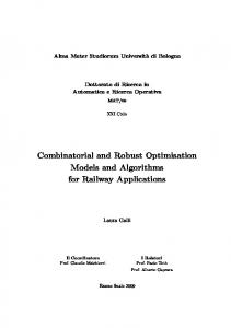
1 X Xj Sn = √ n j=1 will be as following. For small values of n, it will be more or less arbitrary, and for growing values of n up to some number N , it becomes closer and closer to the Gaussian distribution (the tail does not play too essential a role). After the moment N , the distribution of Sn deviates from the Gaussian (the role of the tail is now essential). Let us illustrate this graphically. Suppose that X1 , X2 , . . . , Xn are i.i.d. random variables with density function √ p(x) = (1 − ε)q(x 2) + εs(x). Here q(x) = exp(−|x|)/2 and s(x) = 1/(π(1 + x2 )) are the Laplacian and the Cauchy densities, respectively. Choose ε = 0.01. In panels a through e of Figure 1.1 we show the plot of the density of the sum n

1 X Xj Sn = √ n j=1 (the solid line) versus one of the density of the standard Gaussian distribution (the dashed line). For n = 5 (panel a), we see that the densities are not too close to each other. When n = 10 (panel b), the two densities become closer to each other compared to when n = 5. They are almost identical when n = 25 (panel c). However, the two densities are not as close when n = 50 (panel d) and when n = 100 (panel e). Thus we see that the optimal N is about 25.

6

1

Ill-posed problems 0.4

0.4

0.3

0.3

a 0.2

b

0.1

0.1

0.0

0.0 -3

c

0.2

-2

-1

0

1

2

3

0.4

0.4

0.3

0.3

0.2

d

0.1

-3

-2

-1

0

1

2

3

-3

-2

-1

0

1

2

3

1

2

3

0.2

0.1

0.0

0.0 -3

-2

-1

0

1

2

3

-3

-2

-1

0.4

0.3

e

0.2

0.1

0.0 0

Figure 1.1. Density of a sum with different n versus Gaussian density A very similar result is realized when the comparison is to a stable distribution. Suppose that X1 , X2 , . . . , Xn are i.i.d. random variables with density function p(x) = (1 − ε)q(2x) + εs(x). Here q(x) is a density with ch.f. (1 + |t|)−2 , which belongs to a region of attraction of the Cauchy distribution and s(x) is the density of the standard Gaussian distribution. We choose ε = 0.03. In panels a and b of Figure 1.2 we show the plot of the density of the normalized sum n

Sn =

1X Xj n j=1

(the dashed line) versus one of the density of the Cauchy distribution (the solid line). Panel a in the figure shows the two densities when n = 5. As can be seen, the densities are not too close to each other. However, as can be seen in panel b, the two densities become much closer to each other when n = 50 Let c and γ be two positive constants, and consider the following semi-distance between random variables X and Y : (1.2)

|fX (t) − fY (t)| . |t|γ |t|≥c

dc,γ (X, Y ) = sup

1

Introduction and motivating examples

7

0.35 0.30 0.30 0.25 0.25 0.20 0.20

a

b 0.15

0.15 0.10

0.10

0.05

0.05

0.00

0.00 -3

-2

-1

0

1

2

-3

3

-2

-1

0

1

2

3

Figure 1.2. Density of a sum for various n (solid line) versus Cauchy density (dashed line)

Here and in what follows FX and fX stand for the cumulative distribution function (c.d.f.) and the characteristic function (ch.f.) of X, respectively. Observe that in the case c = 0, dc,γ (X, Y ) defines a well-known probability distance in the space of all random variables for which d0,γ (X, Y ) is finite3 . Next, recall that Y is a strictly α-stable random variable. If for every positive integer n d

(1.3)

Y1 = Un :=

Y1 + · · · + Yn , n1/α

d

where = stands for equality in distribution and the Yj ’s, j ≥ 1, are i.i.d. copies of Y .4 Let X, Xj , j ≥ 1, be a sequence of i.i.d. random variables such that d0,γ (X, Y ) is finite for some strictly stable random variable Y . Suppose that Yj , j ≥ 1, are i.i.d. copies of Y and γ > α. Then5 d0,γ (Sn , Y ) = d0,γ (Sn , Un ) = sup t

≤ n sup t

n |fX (t/n1/α ) − fYn (t/n1/α )| |t|γ

|fX (t/n1/α ) − fY (t/n1/α )| 1 = γ/α−1 d0,γ (X, Y ). γ |t| n

From this we can see that d0,γ (Sn , Y ) tends to zero as n tends to infinity; that is, we have convergence (in d0,γ ) of the normalized sums of Xj to a strictly α-stable random variable Y provided that d0,γ (X, Y ) < ∞. However, any truncation of the tail of the distribution of X leads to d0,γ (X, Y ) = ∞. Our goal is to analyze the closeness of the sum Sn to a strictly α-stable random variable Y without the assumption about the finiteness of d0,γ (X, Y ), restricting our assumptions to bounds in terms of dc,γ (X, Y ) with c > 0. In this way, we can formulate a general type of a central pre-limit theorem with no assumption on the tail behavior of the underlying random variables. We shall illustrate our theorem providing answers to the problems addressed in Examples 1 and 2 in Section 1.1. 3 See

Zolotarev (1986) and Rachev (1991). Zolotarev (1983a) and Lukacs (1969). 5 See Zolotarev (1983a). 4 See

8

1

Ill-posed problems

2. Central Pre-Limit Theorem In our Central Pre-Limit Theorem we shall analyze the closeness of the sum Sn to a strictly α-stable random variable Y in terms of the following Kolmogorov metric,6 defined for any c.d.f.’s F and G as follows: kh (F, G) := sup |F ∗ h(x) − G ∗ h(x)|. x∈IR

Here, ∗ stands for convolution, and the “smoothing” function h(x) is a fixed c.d.f. 0 with a bounded continuous density function, supx |h (x)| ≤ c(h) < ∞. The metric kh metrizes the weak convergence in the space of c.d.f.’s. The following central pre-limit theorem appeared in Klebanov et al. (1999). Theorem 1.1. (Central Pre-Limit Theorem) Let X, Xj , j ≥ 1, be i.i.d. random Pn variables and Sn = n−1/α j=1 Xj . Suppose that Y is a strictly α-stable random variable. Let γ > α and ∆ > δ be arbitrary given positive constants and let n ≤ α (∆ δ ) be an arbitrary positive integer. Then √ dδ,γ (X, Y )(2a)γ c(h) 2π kh (FSn , FY ) ≤ inf +2 + 2∆a . γ a>0 a n α −1 γ Remark 1.1. If ∆ → 0 and ∆/δ → ∞, then n can be chosen large enough so that the right-hand-side of the above bound is sufficiently small, and we obtain the classical limit theorem for weak convergence to an α-stable law. This result, of course, includes the central limit theorem for weak distance. Proof of Theorem 1.1. For γ > α, dc,γ (Sn , Y ) = dc,γ (Sn , Tn ) (1.4)

|fX (t/n1/α ) − fY (t/n1/α )| 1 c = γ −1 d 1/α ,γ (X, Y ). γ n |t| nα |t|≥c

≤ n sup

α For any ∆ > δ and for all n ≤ ( ∆ δ ) , we have then

d∆,γ (Sn , Y ) ≤

1

dδ,γ (X, Y ). n The above relation can be rewritten in the form |fSn (t) − fY (t)| 1 (1.6) sup ≤ γ −1 dδ,γ (X, Y ). γ α |t| n |t|≥∆ (1.5)

γ α −1

Denote by 1I(t) the indicator function of the interval [−∆, ∆]. Then, |t|γ−1 1 |(1 − 1I(t))fSn (t) − (1 − 1I(t))fY (t)| ≤ γ −1 dδ,γ (X, Y ). |t| nα For any a > 0 define  r  1 for |t| < a, π 1 (2a − |t|) for a ≤ |t| ≤ 2a, (1.8) Vea (t) = a 2 0 for |t| > 2a.

(1.7)

The function Vea (t) is now a Fourier transform of the Vallée-Poussin kernel (1.9) 6 See

Va (x) =

1 cos(ax) − cos(2ax) . a x2

Kolmogorov (1953) and Rachev (1991).

2

Central Pre-Limit Theorem

9

We have Z (1 − 1I(t))

(1.10) IR

fSn (t) − fY (t) e e h(t)Va (t)e−itx dt = t

(1.11) ((FSn ∗ h(x) − FSn ∗ h ∗ U∆ (x)) − (FY ∗ h(x) − FY ∗ h ∗ U∆ (x))) ∗ Va (x), where e h(t) is the ch.f. corresponding to the c.d.f. h and 1 sin(∆x) . 2π x (Note that the Fourier transform of U∆ is the indicator function 1I.) We now obtain U∆ (x) =

sup |((FSn (x) − FSn ∗ U∆ (x)) ∗ h(x) − (FY (x) − FY ∗ U∆ (x)) ∗ h ∗ Va (x)| x

≤

(1.12)

dδ,γ (X, Y ) (2a)γ √ 2π. γ γ n α −1

It is known7 that (1.13)

|FSn ∗ h(x) − FSn ∗ h ∗ Va (x)| ≤ EFSn ∗h(x) (a) ≤ Eh (a),

where EF (a) is the order of the best approximation of the function F by entire functions of finite exponential type a. In our case, h has a bounded density function, so Eh (a) ≤ c(h)/a. Similarly, |FY ∗ h(x) − FY ∗ h ∗ Va (x)| ≤ c(h)/a. From a well-known relation between norms of entire functions of finite exponential type (See, Nikolskii (1977, p. 131)), it follows that sup |(FSn (x) − FY (x)) ∗ h ∗ Va ∗ U∆ (x)| ≤ 2∆a.

(1.14)

x

Combining our estimates, we have √ dδ,γ (X, Y )(2a)γ c(h) + 2 + 2∆a kh (FSn , FY ≤ inf 2π γ a>0 a n α −1 γ α for all n ≤ ( ∆ δ) .

Thus, the c.d.f. of a normalized sum of i.i.d. random variables is close to the corresponding α-stable c.d.f. for “mid-size values” of n. We also see that for these values of n, the closeness of Sn to a strictly α-stable random variable depends on the “middle part” (“body”) of the distribution of X. Remark 1.2. Consider our example of radioactive decay and apply Theorem 1.1 to the centralized time moments, denoted by Xj . If Y is Gaussian, γ = 3, α = 2, ∆ = 10−15 , δ = 10−30 , then for n ≤ 1030 the following inequality holds: √ d10−30 ,3 (X, Y )(2a)3 c(h) √ kh (FSn , FY ) ≤ inf 2π +2 + 2 · 10−10 a . a>0 a 3 n Here, d10−30 ,3 (X, Y ) ≤ 1 in view of the fact that |fX (t) − fY (t)| ∼

A2 t, as t → 0. (Eo2 + Γ2 )2

Thus, we obtain a rather good normal approximation of FSn (x) for “not too large” values of n (n ≤ 1040 ). If c(h) ≤ 1 and n is of order 1040 , then kh (FSn , FY ) is of order 10−5 . 7 See

Nikolskii (1977).

10

1

Ill-posed problems

3. Sums of a random number of random variables Limit theorems for random sums of random variables have been studied by many specialists in such fields as probability theory, queueing theory, survival analysis, and financial econometric theory.8 We briefly recall the standard model: suppose X, Xj , j ≥ 1, are i.i.d. random variables and let {νp , p ∈ ∆ ⊂ (0, 1)} be a family of positive integer-valued random variables independent of the sequence of X’s. Suppose that {νp } is such that there exists a ν-strictly stable random variable Y , that is d

1/α

Y =p

νp X

Yj ,

j=1

where Y, Yj , j ≥ 1, are i.i.d. random variables independent of νp , and Eνp = 1/p. Bunge (1996) and Klebanov and Rachev (1996) independently obtained general conditions guaranteeing the existence of analogues of strictly stable distributions for sums of a random number of i.i.d. random variables. For this type of a random summation model, we can derive an analogue of Theorem 1.1. Pνp Theorem 1.2. Let X, Xj , j ≥ 1, be i.i.d. random variables. Let S˜p = p1/α j=1 Xj . ˜ Suppose that Y is a strictly ν-stable random variable Let γ > α, and ∆ > δ be arδ α ) be an arbitrary positive number bitrary given positive constants, and let p ≥ ( ∆ from (0, 1). Then the following inequality holds: ! ˜ )(2a)γ √ γ d (X, Y c(h) δ,γ kh (FS˜p , FY˜ ) ≤ inf p α −1 2π +2 + 2∆a . a>0 γ a Proof of Theorem 1.2. The proof is similar to that of Theorem 1.1. One only needs to use the following inequality Pνp 1/α n t) − fYn˜ (p1/α t)|P (νp = n) j=1 |fX (p dc,γ (S˜p , Y˜ ) ≤ sup |t|γ |t|≥c |fX (p1/α t) − fY˜ (p1/α t)|Eνp |t|γ |t|≥c

≤ sup

γ = p α −1 dcp1/α ,γ (X, Y˜ ),

at the beginning of the proof and then follow the arguments in the proof of Theorem 1.1. 4. Local pre-limit theorems and their applications to finance Now we formulate our “pre-limit” analogue of the classical local limit theorem.9 8 See Gnedenko and Korolev (1996), Klebanov et al. (1984), Kozubowskii and Rachev (1994), and the references therein. 9 Note that in studies in finance the fit of a theoretical distribution to the empirical one is often done in terms of the densities, rather than in terms of the corresponding c.d.f.’s. That is why, in our view, the local pre-limit and limit theorems are of greater importance in comparison to the classical limit theorems when applied to studies on this type in finance.

5

Pre-limit theorem for extremums

11

Theorem 1.3. (Local Pre-Limit Theorem) Let X, Xj , j ≥ 1, be i.i.d. random variables having aPbounded density function with respect to the Lebesgue measure, n and Sn = n−1/α j=1 Xj . Suppose that Y is a strictly α-stable random variable. ∆ α α Let γ > α, ∆ > δ > 0 and n( ∆ δ ) be a positive integer not greater than ( δ ) . Then √ dδ,γ (X, Y )(2a)γ+1 c(h) kh (pSn , pY ) ≤ inf 2π +2 + 2c(h)∆a , γ −1 a>0 α a (γ + 1) n where pSn and pY are the density functions of Sn and Y , respectively. Thus, the density function of the normalized sums of i.i.d. random variables is close in smoothed Kolmogorov distance to the corresponding density of an α-stable distribution for “mid-size values” of n. The corresponding local pre-limit result for the sums of random number of random variables has the following form. Theorem 1.4. (Local Pre-Limit Theorem for Random Sums) Let X, Xj , j ≥ 1, be i.i.d. random variables having density function with respect to the Pνbounded τ Lebesgue measure. Let S˜τ = τ 1/α j=1 Xj . Suppose that Y˜ is a strictly ν-stable α random variable. Let γ > α, and ∆ > δ > 0, and τ ∈ [( ∆ δ ) , 1). Then the following inequality holds: ! √ dδ,γ (X, Y˜ )(2a)γ γ c(h) −1 kh (pS˜τ , pY˜ ) ≤ inf τ α 2π +2 + 2∆a . a>0 γ a Remark 1.3. Consider now our first example in Section 1.1 concerning Paretostable laws. Following the Mandelbrot (1960) model for asset returns, we view a daily asset return as a sum of a random number of tick-by-tick returns observed during the trading day. We can assume that the total number of tick-by-tick returns during the trading day has a geometric distribution with a large expected value. In fact, the limiting distribution for geometric sums of random variables (when the expected value of the total number tends to infinity) is geo-stable.10 Then, according to Theorem 1.4 from Klebanov, Rachev, Kozubowskii (2006), the density function of daily returns is approximately geo-stable (in fact, it is ν-stable with a geometrically distributed ν). 5. Pre-limit theorem for extremums Let X1 , . . . , Xn , . . . be a sequence of non-negative i.i.d. random variables having the c.d.f. F (x). Denote X1;n = min(X1 , . . . , Xn ). It is well-known that if F (x) ∼ axα as x → 0, then Fn (x) (c.d.f. of n1/α X1;n ) tends to the c.d.f. G(x) of the Weibull law, where ( α 1 − e−ax , for x > 0; G(x) = 0, for x ≤ 0. The situation here is almost the same as in the limit theorem for sums of random variables. It is obvious that the index α cannot be defined using empirical data on c.d.f. F (x), and therefore, the problem of finding the limit distribution G is 10 See

Klebanov et al. (1984).

12

1

Ill-posed problems

ill-posed. Here we propose the pre-limit version of the corresponding limit theorem. As an analogue of dc,γ , we introduce another semi-distance between random variables X, Y : |FX (x) − FY (x)| , κc,γ (X, Y ) = sup xγ x>c where FX and FY are c.d.f.’s of non-negative random variables X and Y . Theorem 1.5. Let Xj , j ≥ 1, be non-negative i.i.d. random variables and X1;n = min(X1 , . . . , Xn ). Suppose that Y is a random variable having the Weibull distribution ( α 1 − e−ax , for x > 0; G(x) = 0, for x ≤ 0 α Let γ > α and ∆ > δ be arbitrary given positive constants, and n < ( ∆ δ ) be an arbitrary positive integer. Then α α Aγ sup |Fn (x) − G(x)| ≤ inf 2e−aA + 2(1 − e−a∆ ) + γ −1 κδ,γ (F, G) . A>∆ nα x>0

A little more rough estimator under the conditions of Theorem 1.5 and ∆ < 1 has the form α 1 1 γ sup |Fn (x) − G(x)| ≤ 2 + γ (log ) α εn + 2(1 − e−a∆ ), εn aα x>0 where 1 εn = γ −1 κδ,γ (F, G). nα To get this inequality, it is sufficient to calculate instead the minimum the corre α1 . sponding value for A = a1 log ε1n Proof of Theorem 1.5. We have 1

1

|F n (x/n α ) − Gn (x/n α )| xγ x>∆

κ∆,γ (Fn , G) = κ∆,γ (Fn , Gn ) = sup 1

1

1 |F (x/n α ) − G(x/n α )| = γ −1 κ∆/n αγ −1 ,γ (F, G) γ α x n x>∆ 1 ≤ γ −1 κδ,γ (F, G) nα ∆ α for n ≤ ( δ ) . So that ≤ n sup

(1.1)

κ∆,γ (Fn , G) ≤

1 n

γ α −1

κδ,γ (F, G).

The inequality (1.1) shows that (1.2)

|Fn (x) − G(x)| ≤ xγ

1 κδ,γ (F, G) γ n α −1

holds for all x ≥ ∆. In particular, Fn (∆) ≤ G(∆) + ∆γ εn . Since Fn (x) ≤ Fn (∆) for 0 ≤ x ≤ ∆, then γ

|Fn (x) − G(x)| ≤ 2G(∆) + ∆γ εn = 2(1 − e−a∆ ) + ∆γ εn

6

Relations with robustness of statistical estimators

13

for 0 ≤ x ≤ ∆. For arbitrary A > ∆ we have from (1.2) ¯ F¯n (A) ≤ G(A) + Aγ ε n , (where we use the notation F¯ (x) = 1 − F (x)) and therefore ¯ |Fn (x) − G(x)| ≤ 2G(A) + Aγ ε n for x ≥ A. But from (1.2) we have sup |Fn (x) − G(x)| ≤ Aγ εn . ∆∆

which complete the proof. 6. Relations with robustness of statistical estimators Let X, X1 , . . . , Xn be a random sample from a population having c.d.f. F (x, θ), θ ∈ Θ (which we shall call “the model” here). For simplicity, we shall further assume that F (x, θ) is a c.d.f. of Gaussian law with θ mean and unit variance, so that F (x, θ) = Φ(x − θ) where Φ(x) is c.d.f. of standard normal law. One uses the observations X1 , . . . , Xn to construct an estimator θ∗ = θ∗ (X1 , . . . , Xn ) of the θ-parameter. The main point in the theory of robust estimation is that any proposed estimator should be insensitive (or weakly sensitive) to slight changes of the underlying model; that is, it should be robust.11 For mathematical formalization of this, we have to clarify two notions. The first one is the idea of how to express the notation of “slight changes of underlying model” in quantitative form. And the second is the idea of the measurement of the quality of an estimator. The most popular definition of the changes of the model in the theory of robust estimation is the following contamination scheme. Instead of the normal c.d.f. Φ(x), is considered G(x) = (1 − ε)Φ(x) + εH(x), where H(x) is an arbitrary symmetric c.d.f.. Of course, for small values of ε > 0, the family G(x − θ) is close to the family Φ(x − θ). Sometimes the closeness of the families of c.d.f.’s is considered in terms of uniform distance between corresponding c.d.f.’s, or in terms of Lévy distance. As to the measurement of the quality of an estimator, then it is an asymptotic variance of the estimator. It is a well known fact that Pn the minimum variance estimator for the parameter θ in a “pure” model x ¯ = n1 j=1 xj is non-robust. From our point of view, it is mostly connected not with the presence of contamination, but with the use of asymptotic variance as a loss function. For not too large n, we can apply Theorem 1.1. It is easy to see that ε dc,γ (Φ(x − θ), G(x − θ)) ≤ 2 γ . c 11 See

Huber (1981).

14

1

Ill-posed problems

Suppose that z1 , . . . , zn is a sample from the population with c.d.f. G(x − θ), and let uj = (zj − θ), j = 1, . . . , n. Denote n

√ 1 X z − θ). uj = n(¯ Sn = √ n j=1 0

For any h(x) with a continuous density function, supx |h (x)| ≤ 1, we have √ ε (2a)γ 1 kh (FSn , Φ) ≤ 2 inf 2π γ γ −1 + + ∆ · a . a>0 δ n2 γ a 2 Here γ > 2, n ≤ ∆ , and ∆ > δ > 0 are arbitrary. It is not easy to find the δ 1 infimum over all positive values of a. Therefore, we set a = ∆− 2 to minimize the sum of the two last terms. Also we propose to find ∆ = εc and δ = εc1 to have ∆1/2 δ = ε1/γ . And, finally, we choose γ to maximize the degree c. The corresponding value is r 2 , γ =2+ 3 and therefore ! √ √ 6 2π2γ 1 √ √ + 2ε 12+ 6 (1.3) kh (FSn , Φ) ≤ 2 , γ n1/ 6 for all n≤ε Here

6√ − 12+7 6

.

√

2π2γ ∼ = 6.269467557, γ √ 1 6 1 √ ∼ > . = 0.08404082058 > 11 12 12 + 6 From (1.3) we see that (for very small ε) the properties of z¯ as an estimator of θ do not depend on the tails of contaminating c.d.f. H for not too large values of the sample size. Therefore, the traditional estimator for the location parameter of the Gaussian law is robust for a properly defined loss function. Note that the estimator of “stability” does not depend on whether c.d.f. H(x) is symmetric or not, though the assumption of symmetry is essential when the loss function coincides with asymptotic variance. Of course, we can obtain a corresponding estimator for both Lévy and uniform distances, but the order of “stability” will be worse. For example, the Lévy distance estimator has the form ! √ √ 30 1 2π2γ √ 60+13 30 √ L(FSn , Φ) ≤ 2 + 3ε γ n 3/10 for all n≤ε

10√ − 60+13 30

where

√

,

30 . 5 We shall not provide here the estimator for uniform distance. γ =2+

7

Statistical estimation for non-smooth densities

15

0.5

0.4

0.3

0.2

0.1

0.0 0.0

0.5

1.0

1.5

2.0

2.5

3.0

Figure 1.3. Plots of distributions of normalized sums One possible objection is that the order of “stability” in (1.3) is very bad. On the one hand, our estimators are not precise. On the other hand, it is related to the “improper” choice of the distance between the distributions under consideration. It would be better to use dc,γ as a measure of closeness of the corresponding model and real c.d.f.’s. If dε,γ (Φ(x − θ), G(x − θ)) ≤ ε, and c(h) ≤ 1, then (1.4)

kh (FSn , Φ) ≤ 4

! √ 1 2 2π + ε4 n

for all n ≤ 1ε , which is superior to (1.3). Probably, the estimator of stability is better for other type of distances. We can support this position with numerical examples. Namely, let X1 , X2 , . . . , Xn be i.i.d. random variables distributed as a mixture of the standard Gaussian distribution (with weight 1 − ε) and Cauchy distribution (weight ε). The uniform distance between distribution F (x, n, ε) of the normalized sum n

1 X Sn = √ Xj n j=1 for ε = 0.01, n = 50 and the standard Gaussian distribution is approximately 0.014. For ε = 0.02, n = 50, this distance is about 0.027. Figure 1.3 provides graphs of F (x, n, ε) − 0.5 for n = 50 and ε = 0 (solid line), ε = 0.01 (dashed line, short intervals), and ε = 0.02 (dashed line, long intervals). We propose the use of models that are close to each other in terms of weak distances. Therefore, we cannot use such loss functions like the quadratic one because the risk of one estimator can become infinite. Therefore, we have to discuss possible choices for the losses. This is a major separate problem in statistics, and we refer the reader to Kakosyan, Klebanov, and Melamed (1984b). 7. Statistical estimation for non-smooth densities Now we shall consider some relations between pre-limit theorems for extremums and statistical estimation for non-smooth densities. A typical example here is a problem of estimation of the scale parameter for a uniform distribution. Let us describe it in more detail.

16

1

Ill-posed problems

Suppose that U1 , . . . , Un are i.i.d. random variables uniformly distributed over interval (0, θ). Based on the data, we have to estimate the parameter θ > 0. It is known that the statistic Un;n = max{U1 , . . . , Un } is the best equivariant estimator for θ. Moreover, the distribution of n(θ − Un;n ) tends to exponential law as n tends to infinity. In other words, the speed of convergence of Un;n to the parameter θ is n1 . But it is known that the speed of convergence of a statistical estimator to the “true” value of the parameter is √1n in the case where there is a smooth density function of the observations.12 Our point here is that it is inpossible to verify based on empirical observations whether a density function has a discontinuity point or not. On the other hand, any c.d.f. having a density with a point of discontinuity can be approximated (arbitrary closely) by a c.d.f. having continuous density. But the speed of convergence for corresponding statistical estimators differs essentially (1/n for the jump case, and √ 1/ n in the continuous case). This means that the problem of asymptotic estimation is ill-posed, and we have a situation that is very similar to that of summation of random variables. Let’s now X1 , . . . , Xn be a sample from a population with c.d.f. F (x/θ), θ > 0 (F (+0) = 0). Consider Xn;n as an estimator for θ, and introduce Zj =

θ − Xj , θ

j = 1, . . . , n.

θ−X

n;n It is obvious that Z1;n = . Therefore, we can apply the pre-limit theorem for θ minimums (Theorem 1.5) to study the closeness of the distribution of the normalized estimator to the limit exponential distribution for the pre-limit case. We have

IPθ {Zj < x} = IPθ {Xj > (1 − x)θ} = 1 − F (1 − x), and we see that the c.d.f. of Zj does not depend on θ. Let us denote by Fz the c.d.f. of Zj . Denote by Fn c.d.f. of nZ1;n , and by G - c.d.f. of the exponential law G(x) = 1 − exp{−x} for x > 0. From Theorem 1.5 in the case of α = 1, we obtain Aγ −A −∆ (1.5) sup |Fn (x) − G(x)| ≤ inf 2e + 2(1 − e ) + γ−1 κδ,γ (Fz , G) A>∆ n x for all n ≤ ∆ δ. Consider an examle, when the c.d.f. of observations has the form F (x) = x for 0 < x ≤ a, where a is a fixed positive number, and F (x) is arbitrary for x > a. In this case, it is easy to verify that 1 κa,2 ≤ . 2 1 1√ Choosing in (1.5) δ = a, ∆ = 4 log a a, and A = 12 log a1 , we obtain that sup |Fn (x) − G(x)| ≤ x log

√

a log

1 a

1

for all n < 41 √aa . In other words, the distribution of normalized estimator remains close to the exponential distribution for not too large values of the sample size, although F does not belong to the attraction domain of this distribution. 12 More

detailed formulations may be found in Ibragimov and Khasminskii (1979).

7


17

0.005 0.004 0.003 0.002 0.001 0.000 0.0

0.2

0.4

0.6

0.8

1.0

Figure 1.4. Simulated points (j/m, 1 − Vj ) 0.005 0.004 0.003 0.002 0.001 0.000 0.0

0.2

0.4

0.6

0.8

1.0

Figure 1.5. Simulated points (j/m, 1 − Uj ) Let us now give some results of numerical simulations. We simulated m = 50 samples of the size n = 1000 from two populations. The first one is uniform on (0, 1), and the second has the following distribution function  0, for x < 0,    x, for ≤ x < 1 − ε, F (x, ε) = 1 5/4  1 − ε1/4 (1 − x) , for 1 − ε ≤ x < 1,    1, for x ≥ 1 with ε = 0.005. So, we had i.i.d. random variables Yi,j , i = 1, . . . , n; j = 1, . . . , m with uniform (0, 1) distribution, and i.i.d. Xi,j with distribution F (x, ε). Denote Vj = maxi Yi,j and Uj = maxi Xi,j . In Figure 1.4 the simulated points (j/m, 1 − Vj ) are shown. The values 1 − Vj are identical to those of the difference between the true value of the scale parameter and the value of the estimator for the “true” model. In Figure 1.5 the simulated points (j/m, 1 − Uj ) are shown. The values 1 − Uj are identical to those of the difference between true value of the scale parameter and the value of the estimator for “perturbed” model. Comparing Figures 1.5 and 1.4 we can see that the simulated results are very similar. We can also compare empirical distributions. We simulated m = 5000 samples of the size n = 200 each from the same populations as before. Now we consider normalized values of the differences between true value of the parameter and its statistical estimators: n(1−Vj ) for the “pure” model, and n(1−Uj ) for the “perturbed”

18

1

Ill-posed problems

1.0

0.8

0.6

0.4

0.2

0.0 0

1

2

3

4

5

Figure 1.6. Graphs of distribution functions of the normalized estimators model. Averaging over all m = 5000 samples, we find empirical distributions of the estimator in both models. Figure 1.6 shows the graphs of distributions of the normalized estimator for the “pure” (solid line) and for the “perturbed” models (dashed line). Of course, the agreement is rather good. Our purpose in this chapter is to study the constraints that are imposed on the model elements in the theory of statistical estimation in the presence of certain conditions that seem to be desirable for the theory or its applications. The results derived here can be viewed in two different ways. On the one hand, we attempt to build an axiomatic theory of statistical estimation; on the other hand, these results can be interpreted as recommendations that would allow an applied statistician to justify the use of some statistical models. Let us move now to the notion of a model in the theory of statistical parameter estimation, and to a more exact formulation of the problem. On a measurable space (X, F), define a family of probability measures {IPθ , θ ∈ Θ}, where Θ - is some abstract set. Let x be an observed value distributed according to one of the laws of IPθ , where the corresponding value of the parameter θ is unknown. The objective is to build an estimator of γ(θ) from the observed value of x, where γ(θ) is some given parametric function that maps the parameter space Θ into IRr . Let Rr denote the σ-algebra of Borel subsets of IRr , and let πr denote the set of probability measures on (IRr , Rr ). We will call an estimator (or to be exact, a randomized estimator) of a parametric function γ, a map δ ∗ from X into πr , giving for each x ∈ X a corresponding probability measure δx∗ (·) on Rr . In doing so, we will always assume that for each A ∈ Rr , the quantity δx∗ (A) is a measurable function of an unknown x. If for each x ∈ X the measure δx∗ is degenerate, then we will talk about a non-randomized estimator of a parametric function γ. We denote such non-randomized estimators of γ with the symbol γ ∗ , supplementing it with various indices if necessary. A randomized estimator can be interpreted in the following way: For an observation x, a probability distribution δx∗ is chosen on (IRr , Rr ). Then, we observe an auxiliary random variable with distribution δx∗ . A value δ of this random variable will be accepted as a final estimator of γ(θ). Among various estimators of a parametric function γ, we would like to chose the best one, in some meaning of the word. To formally measure the quality of an estimator, let us introduce a loss function w = w(s, t). Here, the value w(δ, γ(θ)) denotes the losses incurred when δ is used as an estimator of γ(θ). In doing so, let us naturally assume that

7


19

w(s, t) ≥ 0 and w(t, t) = 0 for s, t ∈ IRr , that is, the losses are always nonnegative, and if the value that is being estimated is obtained precisely, losses do not occur. In the future, we shall always assume that these conditions are satisfied, unless specified otherwise. Let δ ∗ be an estimator of γ. Then, the risk of δ ∗ , corresponding to a family {IPθ , θ ∈ Θ} and loss function w, is the mean loss Rθ (δ ∗ , γ; IPθ ; w) = IEθ

Z

w(δ, γ(θ))dδx∗ (δ) =

IRr

Z

Z dIPθ (x)

X

w(δ, γ(θ))dδ ∗ (δ).

IRr

For brevity, we shall simply talk about “a risk of an estimator δ ∗ ” and we may omit the dependency from certain elements. For example, if the family of distributions, loss function, and parametric function γ are clear from the context, we shall simply write Rθ (δ ∗ ) (or Rθ δ ∗ ) instead of Rθ (δ ∗ , γ; IPθ , w). (Of course, it is always assumed that w satisfies necessary measure conditions, so that the corresponding integrals are well defined. In the future these conditions may not be stated explicitly). Note that although the usual loss functions are maps from IRr × IRr to IR1 , sometimes the so-called matrix loss functions are used.13 Here, however, we will mostly deal with scalar loss functions. If δ estimates the value of γ(θ), then it is natural to assume that losses incurred in such estimation depend on the difference δ − γ(θ), or on the norm |δ − γ(θ)|. For this reason, in many applied problems the loss function w has the form w(s, t) = v(s − t) or w(s, t) = v1 (|s − t|), where v and v1 are non-negative functions taking zero values when the argument itself is zero. Then it is often assumed that v1 (z) increases for z > 0. It should be kept in mind that in many problems, it is convenient to consider estimators that belong to some specified class K∗ . (For example, the set of all non-randomized estimators can be considered as a candidate for K∗ .) In the sequel, we shall assume that estimators that belong to the class of interest have finite risk, unless specified otherwise. Sometimes we may have to examine not just one parametric function γ, but all parametric functions from some set K. In other words, for a given function γ ∈ K its estimator δ ∗ ∈ K∗ , which depends on γ ∈ K, should be proposed. Let us call the family of distributions {IPθ θ ∈ Θ} defined on (X, F), the loss functions w, the set of parametric functions K, and the class of estimators K∗ – the model in a theory of statistical parameter estimation (or simply the “model”). An estimator δ˜∗ ∈ K∗ of a parametric function γ is said to be admissible in the class K∗ if the conditions δ ∗ ∈ K∗ , Rθ δ ∗ ≤ Rθ δ˜∗ for all θ ∈ Θ imply that Rθ δ ∗ = Rθ δ˜∗

for all θ ∈ Θ.

13 Such loss functions were studied in Lebedev et al. (1971), Klebanov et al. (1971), and Linnik and Rukhin (1972).

20

1

Ill-posed problems

Thus, if an estimator δ˜∗ is admissible in the class K∗ , then in this class there is no other estimator whose risk would be uniformly smaller than the risk of δ˜∗ , and there is at least one value of θ for which the risk is strictly less than the risk of δ˜∗ . An estimator δ˜∗ ∈ K∗ is called minimax in class K∗ , if sup Rθ δ˜∗ = inf sup Rθ δ ∗ . θ∈Θ

δ ∗ ∈K∗ θ∈Θ

An estimator δ˜∗ ∈ K∗ is called an optimal estimator of a parametric function γ ∈ K in class K∗ if for any estimator δ ∗ ∈ K∗ , the following inequality holds Rθ δ˜∗ ≤ Rθ δ ∗ , θ ∈ Θ. Clearly, if an estimator δ˜∗ is optimal in class K∗ , then it also is admissible and minimax in K∗ . Let K∗ be some set of estimators, and let K∗1 ⊂ K∗ be a subset of K∗ . Let us say that K∗1 is a complete subset of K∗ if for any estimator δ ∗ ∈ K∗ of a parametric function γ there exists an estimator δ˜∗ ∈ K∗ of the same parametric function such that the following identity holds: Rθ δ˜∗ ≤ Rθ δ ∗ for all θ ∈ Θ. If K∗ is a set of all estimators with finite risks, then we will call its complete subclass a complete class. The main (classical) problem of the theory of statistical estimation consists of finding optimal (or admissible, or minimax) estimators for a given model, and proving optimality and admissibility (or, on the contrary, inadmissibility) of the estimators that seem natural and convenient for some applications. However, we will not be investigating such an issue here. As mentioned before, our aim is to investigate the relationship among the elements of the model in the theory of statistical estimation, and to study how certain conveniences that seem to be natural impose limitations on the model. Under such conveniences, we can understand, for example, the requirement of: 1. Completeness of a class of non-randomized estimators; 2. Completeness of a class of estimators that are symmetric functions of observations obtained via repeated sampling scheme; 3. The use of “difference” loss functions w(s, t) = v(s − t) or w(s, t) = v1 (|s − t|), with preservation of a possibility to improve any estimator by a function of a sufficient statistic; 4. Many other conditions. Observe that even when studying the main problem of the theory of statistical estimation one has to remember that in practice a model (or some of its elements) can be known only approximately. This is why it is desirable to investigate how the change of certain model elements affects the quality of estimators. Our main interest here is in construction of “stable” models, that is models for which small (in some sense of this word) changes of their elements lead to small changes in a quality of estimators in use. Note that not all models are stable in such a sense. Recommendations on how to build stable models are part of this book as well.

8

Key points of this chapter

21

The three requirements enumerated above are connected mostly to the problem of selecting a loss function. In addition, the question of model building contains in itself the issue of selecting the distribution family, which in essence is an issue of describing all changes that satisfy certain desirable statistical properties. Consequently, the part of model building related to the selection of a family of distributions, is also closely related to a fast developing field of probability theory and mathematical statistics called problems of characterizations. For this reason, we shall propose one fairly general method for proving characterization theorems (not necessarily related to estimation problems) and illustrate its possibilities when applied to certain concrete results. This method utilizes a relatively new notion of an intensively monotone operator. It turns out that for functional equations that have intensively monotone operators, uniqueness theorems can be established fairly easily. Derivations of certain characterization theorems can be reduced to proving the uniqueness of the solution of a functional equation, and this fact stipulates the applicability of the intensively monotone operator method to characterization problems. Construction of “stable” models is clearly related to the investigation of stability in characterization problems and, therefore, to the rapidly developing theory of stability of stochastic models.14 Of course this connection is not only limited to the investigation of stable characterizations, but also comes up in the selection of loss functions and in building “stable” methods for parametric function estimation. Characterization problems in statistics and the theory of stable stochastic models is the link between the problem of model building in the theory of estimation and the theory of integral (and general functional) equations and inequalities and functional analysis along with the theory of probability measures. The issue of describing “natural” loss functions has implications in game theory, which will be mentioned briefly at the end of Chapter 2. 8. Key points of this chapter • Practitioners typically deal with problems with a finite sample, calling into question the applicability of limit theorems in modeling some effects in probability and statistics. • In many situations, pre-limit theorems seem to be more suitable for probabilistic modeling • Classical statistical methods are usually robust for small deviations from the model if the inference is based on distributional properties for a fixed number of observations. • To measure the quality of a statistical procedure, one needs some special definitions of a loss function.

14 See, for example, Khalfin and Zolotarev (1976), Khalfin and Zolotarev (1979), and Zolotarev and Kalashnikov (1980,1981,1983).

22

1

Ill-posed problems

CHAPTER 2

Loss functions and the restrictions imposed on the model 1. Introduction The basic objective of the statistical theory of parameter estimation is that it does not have an accurate mathematical meaning until we define the notion of the “best” estimator. As it is often the case with prolific mathematical concepts, the foundations of a general theory of statistical inference appears in the work of Gauss and even earlier in the work of Laplace. We quote here from Jerzy Neyman’s lecture Basic Problems of Mathematical Statistics,1 where he describes the origins of the concept of the loss function: “In order to rationalize the choice of an estimator θ∗ (x), Laplace considered the process of estimation as a game in which statistician can win anything but can lose a lot because of the estimation error. Laplace was aware of the fact that the choice of a measure of this error should be subjective, and he has chosen the absolute value of the difference between the true value of a parameter θ and the estimator θ∗ (x). The mean value of this loss function, Z Rθ (θ∗ (x)) = |θ∗ (x) − θ|dFθ (x), is called the risk function corresponding to the estimator θ∗ (x), and constitutes the basis for comparison of the accuracy of this estimator depending on particular values of the parameter θ. Gauss followed a path which was analogous to the one chosen by Laplace. He noticed that in many problems one can simplify considerations if the loss function of Laplace is replaced by its square |θ∗ (x) − θ|2 . This replacement led to the introduction of the least squares method.” In this chapter,2 we attempt to demonstrate that a choice of a loss function is by no means subjective and that the loss function introduced by Gauss (the quadratic loss function), despite the simplicity of the formula, has certain deficiencies when compared to the Laplace’s loss function. The main goal of this chapter is to show what properties of loss functions warrant a complete class of “natural” estimators. In order to describe these loss functions, we need several new notions which are introduced in the next section. 1 Neyman 2 Some

(1961). of the results were obtained in Klebanov and Gupta (2001). 23

24

2

Loss functions and the restrictions imposed on the model

2. Reducible families of functions We shall first introduce the notion of a reducible family of functions, which strengthens the notion of a convex function. Let {Wt (·), t ∈ T } be a family of real functions of a real argument, where T is a certain abstract set.3 Definition 2.1. We say that {Wt (·), t ∈ T } is a reducible family of functions if for each cumulative distribution function G(s) on IR1 there exists a point s∗ = s∗ (G) such that Z (2.1) Wt (s)dG(s) ≥ Wt (s∗ ), ∀t ∈ T, IR1

assuming that the integral on the left hand side exists and is finite. We also assume that s∗ is a measurable function of G.4 If in Definition 2.1 instead of the existence of s∗ we required the equality Z ∗ S = sdG(s), IR1

then (2.1) would reduce to Jensen’s inequality and would be equivalent to convexity of each function Wt (s) from the given family. Instead, if the family consists of one continuous function Wt0 (s) attaining its minimum and maximum values, then by the mean-value theorem, Z Wt0 (s)dG(s) = Wt0 (s∗ ) IR1

without any convexity conditions. Next, we formulate three more definitions related to the one above. Definition 2.2. We say that {Wt (·), t ∈ T } is a strongly reducible family of functions if it is a reducible family and the inequality (2.1) is strict for each nondegenerate c.d.f. G(s). Definition 2.3. We say that {Wt (·), t ∈ T } is a weakly reducible family of functions if for each two real numbers s1 , s2 and each rational p ∈ (0, 1) there exists a point s∗ = s∗ (s1 , s2 ; p) such that (2.2)

pWt (s1 ) + (1 − p)Wt (s2 ) ≥ Wt (s∗ ), ∀t ∈ T,

where s∗ is a measurable function of s1 and s2 . Definition 2.4. We say that {Wt (·), t ∈ T } is a continuously weakly reducible family of functions if 1. The functions Wt (s) are continuous; 2. The family is weakly reducible ; 3. The point s∗ satisfying (2.2) can be chosen in such a way that it becomes a continuous function of s1 , s2 , and p. Clearly, if {Wt (·), t ∈ T } is reducible, then it is weakly reducible. However, the opposite implication is not true in general. 3 For

these four definitions, see Klebanov (1984). of s∗ as a function of G is understood here in the following sense. Let Gu (s) be a family of c.d.f.’s which is a measurable function of u for each fixed s ∈ IR1 . Then we assume that s∗ (Gu ) is also a measurable function of u. 4 Measurability

2

Reducible families of functions

25

2.1. Weakly Reducible Families. Consider the following example. Example 2.1. Let T = {1, 2, 3} and 1 , W1 (s) = 0 , 0 , W2 (s) = s , 0 , W3 (s) = −s ,

if s is irrational, if s is rational, if s is irrational, if s is rational, if s is irrational, if s is rational.

Then, the family {Wt (·), t ∈ T } is weakly reducible but not reducible. Proof of Example 2.1. We need to define s∗ satisfying (2.2). If s1 and s2 are irrational numbers, and p ∈ (0, 1) is an arbitrary rational number, then we can take for s∗ (s1 , s2 ; p) an arbitrary irrational number or zero. If s1 and s2 are rational, then it is easy to see that (2.2) holds if and only if s∗ is rational and s∗ = ps1 (equivalently s∗ = (1 − p)s2 ). If this family was reducible, then equation (2.2) should be satisfied for rational s1 and s2 and irrational p. But for rational s1 and s2 and t = 1 we should have W1 (s∗ ) ≤ 0, i.e., s∗ should be rational. For t = 2 we find that ps1 + (1 − p)s2 ≥ s∗ , and for t = 3, −(ps1 + (1 − p)s2 ) ≥ −s∗ , i.e., s∗ has the form s∗ = ps1 + (1 − p)s2 , which, in view of the irrationality of p, leads to a contradiction with the rationality of s∗ . Let us formulate here one simple result which establishes an equivalent condition to the weakly reducible family of functions. Theorem 2.1. A family {Wt (·), t ∈ T } is weakly reducible if and only if for each integer n ≥ 2 and each choice of real numbers s1 , . . . , sn there exists a point s∗n = s∗n (s1 , . . . , sn ), which is a measurable function of s1 , . . . , sn and such that n

(2.3)

1X Wt (sj ) ≥ Wt (s∗n ), ∀t ∈ T. n j=1

Proof of Theorem 2.1. Assume that the family {Wt (·), t ∈ T } is weakly reducible. We shall prove by induction that (2.3) holds. Indeed, taking p = 1/2 in (2.2) we obtain (2.3) for n = 2. If (2.3) holds for some n ≥ 2, then n+1 1 X Wt (sj ) ≥ n + 1 j=1

n 1 Wt (s∗n ) + Wt (sn+1 ) n+1 n+1

≥ W (s∗ (s∗n , sn+1 ; n/(n + 1))). Thus (2.3) follows by induction.

26

2


Conversely, if the family {Wt (·), t ∈ T } satisfies (2.3) for all n ≥ 2 and p ∈ (0, 1) is a rational number of the form k/n, then by choosing in (2.3) the first k numbers among sj ’s equal to s0 and the remaining n − k equal to s00 , we obtain k k Wt (s0 ) + (1 − )Wt (s00 ) ≥ Wt (s∗n (s0 , . . . , s0 , s00 , . . . , s00 )), n n which coincides with (2.2). Remark 2.1. Clearly, s∗n in (2.3) can be chosen to be a symmetric function of arguments s1 , . . . , sn . We demonstrate that a continuous weakly reducible family satisfying some additional conditions becomes reducible. Theorem 2.2. Let a family {Wt (·), t ∈ T } be continuously weakly reducible. Assume that for each t ∈ T there exist (finite of infinite) limits lims→∞ Wt (s) and lims→−∞ Wt (s), and (2.4)

lim Wt (s) = lim Wt (s) > Wt (x)

s→∞

s→−∞

1

for all x ∈ IR . Then the family {Wt (·), t ∈ T } is reducible. Proof of Theorem 2.2. The following property is easy to show by induction: If the family {Wt (·), tP ∈ T } is weakly reducible, then for all real numbers n p1 , . . . , pn satisfying pj ≥ 0, j=1 pj = 1, there exists a point s∗n = s∗n (s1 , . . . , sn ; p1 , . . . , pn ) such that

n X

pj Wt (sj ) ≥ Wt (s∗n ), ∀t ∈ T.

j=1 (n)

(n)

Now, let G(s) be an arbitrary c.d.f. We can select sj , pj , (j = 1, . . . , n) in such a way that for all t ∈ T the following condition is satisfied Z n X (n) (n) lim Pj Wt (sj ) = Wt (s)dG(s). n→∞

IR1

j=1

Let us consider the sequence of resulting points s∗n , n = 1, 2, . . . . We demonstrate that it is bounded. Indeed, if there exists a subsequence s∗nk for which limk→∞ |s∗nk | = ∞, then by (2.4) we would have lim Wt (s)

s→±∞

=

lim Wt (s∗nk ) ≤ lim

k→∞

k→∞

nk X

(nk )

pj

(nk )

Wt (sj

)

j=1

Z =

Wt (s)dG(s) < lim Wt (s). s→±∞

IR1

This is a contradiction and thus {s∗n }∞ n=1 is bounded. ∗ ∞ Now, consider a subsequence {s∗nl }∞ l=1 of the sequence {sn }n=1 ∗ vergent to some point s . By the continuity of Wt (s) we have Wt (s∗ )

= ≤

lim Wt (s∗nl )

l→∞

lim

l→∞

nl X j=1

(nl )

pj

(nl )

Wt (sj

Z )=

Wt (s)dG(s). IR1

which is con-

2


27

2.2. Reducible Families. For classes obtained by shifting some functions, the reducible property becomes the equivalent of convexity. Here is a precise formulation of this result. Theorem 2.3. Let v(s) be a positive, even, and locally integrable function on IR1 such that for each ε > 0 there exists δ = δ(ε) > 0 such that inf{v(s) : |s| ≥ ε} > v(0) + δ.

(2.5)

In order for the family {v(s − t), t ∈ IR1 } to be weakly reducible it is necessary and sufficient that the function v be convex. Proof of Theorem 2.3. If the function v is convex, then pv(s1 − t) + (1 − p)v(s2 − t) ≥

v(p(s1 − t) + (1 − p)(s2 − t))

= v(ps1 + (1 − p)s2 − t) and condition (2.2) is satisfied with the function s∗ = ps1 +(1−p)s2 , i.e., the family {v(s − t), t ∈ IR1 } is weakly reducible. Now, let us assume that the family {v(s − t), t ∈ IR1 } is weakly reducible. First we show the convexity of the function v under the additional assumption that it is continuously differentiable. We demonstrate that if a positive twice continuously differentiable function v satisfies (2.5) and it is not convex, then there exists a point ξ for which v 0 (ξ) > 0 and v 00 (ξ) < 0. Indeed, let U = {s ≥ 0 : v 0 (s) > 0}. By (2.5), U 6= ∅. We need to show that for some ξ ∈ U , v 00 (ξ) < 0. Assume the opposite, i.e., v 00 (s) ≥ 0 for all s ∈ U . Since v 0 is continuous, for each point s0 ∈ U there exists an interval (α, β) such that s0 (α, β) ⊆ U . Let [a, b] be a maximal interval satisfying the following 1. (α, β) ⊆ [a, b]; 2. v 00 (s) ≥ 0 for all s ∈ [a, b]. Since v 0 (s0 ) ≥ 0 and v 00 (s) ≥ 0 for s ∈ [a, b], v 0 (s) > 0 for s ∈ [s0 , b], i.e., [s0 , b] ⊆ U . In particular, if b < ∞, then v 0 (b) > 0. Therefore, [b − η, b + η] ⊆ U for some η > 0. However, by the assumptions, v 00 (s) ≥ 0 for s ∈ U , and thus also for s ∈ [b, b + η], which contradicts that [a, b] was maximal. This contradiction does not hold only if b = ∞. In this way, the interval [s0 , ∞) ⊆ U for each s0 ∈ U . Set γ = inf U , so U = (γ, ∞). From (2.5) it follows that the function v should have points of increase in an arbitrary small neighborhood of zero, i.e., γ = 0. Thus the positive function v should be convex which is in contradiction with the assumption. We have thus shown existence of ξ: v 0 (ξ) > 0, v 00 (ξ) < 0 (ξ > 0). Assume now that the positive twice differentiable function v satisfying (2.5) is not convex and the family {v(s − t), t ∈ IR1 } is weakly reducible. In this case, we can find numbers ξ > 0 and ε0 , 0 < ε0 < ξ such that v 0 (s) > 0, v 00 (s) < 0 for [ξ − ε0 , ξ + ε0 ]. Let δ0 > 0 satisfy the condition inf{v(s) : |s| ≥ ε0 /2} > v(0) + δ0 .

28

2


Consider the points s2 , 0 < s2 < min(ε0 , δ0 ), and s1 = −s2 . Since the family {v(s − t), t ∈ IR1 } is weakly reducible, we should have (2.6)

1 (v(s1 − t) + v(s2 − t)) ≥ v(s∗ − t), t ∈ IR1 2

for some s∗ , which depends of s1 and s2 . Substituting in (2.6) t = 0, we see that v(0) ≤ v(s∗ ) < v(0) + δ0 . Thus, ∗ |s | ≤ ε0 /2 and s1 − ε0 /2 < s∗ < s2 + ε0 /2. We now substitute in (2.6) t = −ξ, so that the points s1 − t, s2 − t, s∗ − t belong to the interval [ξ − ε0 , ξ + ε0 ]. In this interval, the function v is concave and increasing. Thus, in order for (2.6) to hold with t = −ξ, it is necessary that s∗ − t

1 ((s1 − t) + (s2 − t)), 2

and so s∗ > 0. Thus, we obtain a contradiction with (2.7), derived from the assumption that v is not convex. So far we have shown that the weak reducible property of the family {v(s−t), t ∈ IR1 } implies the convexity of the function v under the additional assumption that the function v is twice continuously differentiable. To prove the theorem in full generality it is enough to smooth the function v. Namely, let ωρ (x) ≥ 0 be an infinitely differentiable function satisfying the conditions: ωρ (x) = 0 if |x| ≥ ρ, R∞ ω (x)dx = 1 (ρ > 0). Since the family {v(s − t), t ∈ IR1 } is weakly reducible, ρ −∞ for each s1 , s2 and rational p ∈ (0, 1), we have (2.8)

pv(s1 − t) + (1 − p)v(s2 − t) ≥ v(s∗ − t), ∀t ∈ IR1 ,

where s∗ depends only on s1 , s2 , and p. We multiply both the sides of (2.8) by ωρ (t − τ ) and integrate with respect to t over the interval (−∞, ∞) to obtain (2.9)

pvρ (s1 − τ ) + (1 − p)vρ (s2 − τ ) ≥ vρ (s∗ − τ ), ∀τ ∈ IR1 ,

where Z

∞

v(θ)ωρ (z − θ)dθ.

vρ (z) = −∞

Obviously, vρ (z) is a infinitely differentiable function and vρ (z) → v(z) when ρ → 0 for almost all z. Condition (2.9) means that the family {vρ(s − t), t ∈ IR1 } is weakly reducible and it is clear that (for sufficiently small ρ > 0) this family satisfies condition (2.5). By the previous argument, the function vρ (z) is convex and consequently so is v(z) (as a limit of convex functions).

2


29

2.3. Strongly Reducible Families. We shall now consider strongly reducible families generated by shifts. Theorem 2.4. Let v(s) be a positive, even, and locally integrable function on IR1 , satisfying condition (2.5). The family {v(s − t), t ∈ IR1 } is strongly reducible if and only if the function v is strongly convex. Proof of Theorem 2.4. If the function v(s) is strongly convex, then the family {v(s − t), t ∈ IR1 } is strongly reducible by Jensen’s inequality. Assume now that the family {v(s−t), t ∈ IR1 } is strongly reducible. Since strong reducibility implies weak reducibility, by Theorem 2.3 the function v is convex. We shall prove that v cannot have linear components. Assume the opposite and let v(x) = ax + b for x ∈ [α, β], where 0 < α < β. From the definition of strongly reducibility, it follows that for each continuous c.d.f. G on IR1 there exists a point s∗ = s∗ (G) such that Z v(s − t)dG(s) > v(s∗ − t), ∀t ∈ IR1 . IR1

Let a c.d.f. G be concentrated with equal probability at two points s1 and s2 , where s2 = −s1 = s, 0 < s < (β − α)/2. The last equality for this choice of G takes the form (2.10)

v(s − t) + v(−s − t) > 2v(s∗ − t), ∀t ∈ IR1 .

For t = 0, by (2.10) and the positivity of v, we have v(s∗ ) < v(s), so that −s < s∗ < s and v(z) is monotone for z ≥ 0. By taking t = −(α + β)/2 in (2.10), the linearity of v on (α, β) implies a(s + (α + β)/2) + a(−s + (α + β)/2) + 2b

> 2a((α + β)/2 + s∗ ) + 2b,

that is, s∗ < 0. But for t = (α + β)/2, it follows from (2.10) by an analogous argument that s∗ > 0. This contradiction proves strong convexity of the function v. 2.4. Reducible and Non-Reducible Families. Now shall now present several examples of reducible and non-reducible families. Example 2.2. It is clear that an arbitrary family {vt (s), t ∈ T } of convex and real functions on IR1 is reducible. Example 2.3. Let {vt (s), t ∈ T } be an arbitrary family of functions defined on the same interval (a, b), and convex on this interval. Assume that a function h is a one-to-one mapping of IR1 on (a, b). Then the family {wt (s), t ∈ T }, where wt (s) = vt (h(s)), is reducible. Proof of Example 2.3. Let G(s) be an arbitrary c.d.f. for which there exists the integral Z wt (s)dG(s). IR1

30

2


Set s∗ = h−1 (

Z h(s)dG(s)). IR1

By Jensen’s inequality, we have for vt (s): Z Z Z wt (s)dG(s) = vt (h(s))dG(s) ≥ vt ( h(s)dG(s)) = wt (s∗ ), ∀t ∈ T. 1 1 1 IR IR IR R The existence of the integral IR1 h(s)dG(s) follows. Clearly, one can obtain examples of reducible families characterizing functions that are not convex in any rational sense. Example 2.4. Let {wt (s), t ∈ T } be a family of functions that achieve the minimum at the same point s∗ (not dependent on t). It is clear that this is a reducible family. Example 2.5. Let w(z) = |z|. Then, it follows from Theorem 2.4 that the family {w(s − t), t ∈ IR1 } is reducible but not strongly reducible. Example 2.6. For a > 0, let 0 w(z) = 1

for for

z ∈ (−a, a), z∈ / (−a, a).

Then, the family {w(s − t), t ∈ IR1 } is not weakly reducible. Note that this result is not a consequence of Theorem 2.3 since (2.5) does not hold. Proof of Example 2.6. Let G(s) be the c.d.f. of a random variable taking on values −a/2 and a/2 with probabilities 1/2 each. If the above family was weakly reducible then we should have (2.11)

(w(−a/2 − t) + w(a/2 − t))/2 ≥ w(s∗ − t)

for some values of s∗ (not depending on t) and all t ∈ IR1 . Let us first take t = −a in (2.11). Here, we have 1/2 ≥ w(s∗ + a), so that ∗ s + a < a and s∗ < 0. Now, put t = a in (2.11) to obtain 1/2 ≥ w(s∗ − a), i.e., s∗ − a > −a, s∗ > 0. The obtained contradiction concludes the proof. 3. The classification of classes of estimators by their completeness types In this section we shall again consider sampling with replacement, so that (n)

X = Xn = X n , A = An = An , Pθ = Pθ

= Qθ × · · · × Qθ ,

where {Qθ , θ ∈ Θ} is a family of probability measures on the measurable space (X, A). For x ∈ X we write x = (x1 , . . . , xn ), where xj ∈ X. Thus, the vector x consists of n independent and identically distributed observations x1 , . . . , xn . 3.1. Completeness Properties. Below we define four completeness properties for classes of estimators and then investigate their mutual relations: Property 1: Completeness of Information Property 2: Lack of Randomization Condition Property 3: Symmetrization Condition Property 4: Rao-Blackwell Condition. Property 1: Completeness of Information: Assume that we have an estimator ∗ δn−1 of a certain parameter function γ : Θ → IR1 , based on n − 1 observations

3

The classification of classes of estimators by their completeness types

31

x1 , . . . , xn−1 . We want to know whether given n observations x1 , . . . , xn , one can (n) ∗ obtain an estimator δn∗ which is better than δn−1 for each measure Pθ , i.e., for which the following inequality would hold (2.12)

(n)

(n−1)

∗ Rθ (δn∗ , γ; Pθ ; w) < Rθ (δn−1 , γ; Pθ

; w), ∀θ ∈ Θ.

In other words, we would like to know whether the new observation xn contains information about the parameter function γ which could be exploited for reducing the risk of estimation of this parameter function. (n−1) ∗ Clearly, if for some θ0 ∈ Θ the estimator δn−1 is constant with Pθ0 -probability ∗ one5 and δn−1 = γ(θ0 ), then (n−1)

∗ Rθ0 (δn−1 , γ; Pθ0

; w) = 0,

and thus the risk of such an estimator cannot be essentially reduced. Thus, we ∗ are interested in improving only the estimators δn−1 that are not constant. This approach is quite general, as estimators that are constant in the above sense are not very useful. If in (2.12) we fix all elements of the model except the loss function, then the obtained property becomes a property of the loss function which characterizes a possibility of reducing the risk by using the information provided by the n-th observation. This is reflected in the following definition.6 Definition 2.5. We say that a loss function w satisfies the condition of complete information (CI condition), if for each family of distributions {Qθ , θ ∈ Θ}, each integer n ≥ 2, each parameter function γ, and an arbitrary random estima(n−1) ∗ ∗ tor δn−1 (δn−1 6= const Pθ –almost surely for each θ ∈ Θ) based on n − 1 observations, there exists an estimator δn∗ based on n observations for which inequality (2.12) holds. The CI condition says that in order to construct “good” estimators one should use all available observations. On the other hand, using the loss function that does not satisfy the condition of complete information does not seem plausible. In extreme cases it may require additional assumptions and can lead to ignoring some of (equally important) observations. Property 2: Lack of Randomization Condition: Randomized estimators require an additional random mechanism. At first glance, it appears that such mechanism should often lead to reduction of estimation accuracy, making it useless. Although this statement is in general incorrect, it is interesting to explain situations in which this actually occurs. We again want to modify the property of completeness of the class of non-randomized estimators so it will be related only to a loss function. The following definition appeared in Klebanov (1981a): Definition 2.6. We say that a loss function w satisfies the condition of lack of randomization (LR condition), if for each family of distributions {Pθ , θ ∈ Θ}, each parameter function γ and an arbitrary randomized estimator δ ∗ there exists 5 We

(n−1)

∗ say that δn−1 is constant with Pθ

∗ concentrated at some point γn−1 (x) and 6 See Klebanov (1979a, 1981a).

0

∗ -probability one if δn−1 is a degenerated measure

(n−1) ∗ Pθ {γn−1 (x) 0

= const } = 1.

32

2


∗ an estimator γ ∗ which belongs to the class Kn.r. of all non-randomized estimators and such that

(2.13)

Rθ (γ ∗ , γ; Pθ ; w) ≤ Rθ (δ ∗ , γ; Pθ ; w), ∀θ ∈ Θ.

In other words, for each randomized estimator, there exists a non-randomized one with a smaller (or equal) risk. Consequently, one can restrict attention to non-randomized estimators (for an arbitrary family of distributions). Property 3: Symmetrization Condition: Consider only non-randomized estimators based on a random sample of size n. Since the observations x1 , . . . , xn are in some sense equivalent (since they are independent and identically distributed), it seems reasonable to consider only estimators that symmetric functions of the observations x1 , . . . , xn . To address this we introduce the following definition.7 Definition 2.7. We say that a loss function w satisfies the condition of symmetrization (S condition), if for each family of probability measures {Pθ , θ ∈ Θ}, an integer n ≥ 2, parameter function γ and its non-randomized estimator γ ∗ : Xn → ∗ IR1 , there exists a statistic γˆ ∗ ∈ Kn.r. , symmetric with respect to the coordinates of x = (x1 , . . . , xn ), such that (2.14)

(n)

(n)

Rθ (ˆ γ ∗ , γ; Pθ ; w) ≤ Rθ (γ ∗ , γ; Pθ ; w), ∀θ ∈ Θ.

The S-condition can be interpreted in the following way: A “good” assessment of the value of γ(θ) should be independent of the order in which the observations were received from measurement devices (or observers) and then statistically analyzed. Property 4: Rao-Blackwell Condition: The last requirement is a certain strengthening of the S condition and is referred to as the Rao-Blackwell (RB) condition. Let {Pθ , θ ∈ Θ} be a family of probability measures on a measurable space (X, A) for which there exists a sufficient statistics T for the parameter θ ∈ Θ.8 Below, when referring to sufficiency in the RB condition, we assume that for considered families there exists a regular conditional probability given a value of the sufficient statistics T . If a loss function w(s, t) is convex in s for each fixed t, then by the Rao-Blackwell theorem,9 non-randomized estimators which are functions of the sufficient statistic T constitute a complete subclass of the class of all non∗ randomized estimators Kn.r. . The Rao-Blackwell theorem does not say anything about the necessity of convexity of w(s, t) in s. Thus, it is of interest to describe the loss functions for which an analog of the Rao-Blackwell theorem holds, i.e., loss functions satisfying the following definition: Definition 2.8. We say that a loss function w satisfies the Rao-Blackwell condition (RB condition), if for an arbitrary measurable space (X, A) on which there is defined a family of distributions {Pθ , θ ∈ Θ} having a sufficient statistics T , and for an arbitrary non-randomized estimator γ ∗ of parameter function γ, there exists a non-randomized estimator γ˜ ∗ of the same parameter function which depends only on the sufficient statistic T and such that (2.15) 7 See

Rθ (˜ γ ∗ , γ; Pθ ; w) ≤ Rθ (γ ∗ , γ; Pθ ; w) ∀θ ∈ Θ.

Klebanov (1975a, 1975b). the definition and a motivation of sufficiency, see Lehmann (1959) and Klebanov (1973a). 9 Rao (1945) and Blackwell (1947). 8 For

3


33

Clearly, if a loss function w satisfies the RB condition, then it also satisfies the S-condition. 3.2. Loss Functions Satisfying the Four Conditions. Note that requiring that one of the above four conditions is satisfied, in a sense, reduces the role of “randomness” in estimation. The CI-condition means that the addition of a new observation can be used for reduction of the role of randomness by reducing the estimation risk. The LR-condition discards additional random mechanism in the construction of an estimator. The S-condition rejects randomness related to the order of obtaining data. The RB-condition allows for rejection of the non-informative component in the selection, since sufficient statistics “contains all information” about a considered family. There exist theorems stating that in the scheme of sampling with replacement, symmetric randomized estimators constitute a complex class. From our point of view, this is not essential, since randomness related to the order in which data are obtained is equivalent to the random mechanism used for computation of the value of an estimator. Thus, through Definitions 2.5-2.8, we have introduced four properties of the loss function, induced by the conditions of completeness of certain classes of estimators. We now turn to the description of the loss functions satisfying these conditions. The following result appeared in Klebanov (1984): Theorem 2.5. Let a loss function w satisfy one of the following conditions a. sups,t w(s, t) < ∞; b. for each s1 ≥ s2 ≥ t ≥ s3 ≥ s4 the following conditions are satisfied w(s1 , t) ≥ w(s2 , t), w(s4 , t) ≥ w(s3 , t), sup w(s, t) = ∞. s

Then the function w(s, t) satisfies the CI-condition if and only if the family {w(s, t), t ∈ IR1 } is strongly reducible. Proof of Theorem 2.5. First, we assume that w(s, t) satisfies the CI-condition and show that the family {w(s, t), t ∈ IR1 } is strongly reducible. We need to demonstrate that for an arbitrary continuous c.d.f. G(δ) on IR1 there exist a degenerated c.d.f. H(δ) concentrated at a point γ ∗ which depends on G and such that for all t ∈ IR1 Z Z (2.16) w(δ, t)dG(δ) > w(δ, t)dH(δ) = w(γ ∗ , t). IR1

IR1

Indeed, let X = {0, 1} and let A be a set of all subsets of X. Set X = X 2 , Pθ = Qθ × Qθ , x = (x1 , x2 ) ∈ X. Let G1 (δ) be an arbitrary non-degenerated c.d.f. on IR1 , and let γ(θ) be an arbitrary (temporarily) parameter function. We assume that an estimator δ1∗ is such that for x = 1 it induces on IR1 a distribution which coincide with G1 (δ) and in other cases it is arbitrary but not constant almost everywhere with respect to measures Qθ , θ ∈ [0, 1]. By the complete information condition, there exists an estimator δ2∗ : X → Π1 for which (2.17)

Rθ (δ2∗ , γ; Pθ ; w) < Rθ (δ1∗ , γ; Qθ ; w), θ ∈ [0, 1].

Set θ = 0. The measure Q0 is concentrating at the point {1}, while the measure P0 at the point {1, 1}. If δ2∗ with x = (1, 1) is inducing the distribution G2 (δ) on

34

2


IR1 , then inequality (2.17) produces Z Z (2.18) w(δ, t)dG1 (δ) > IR1

w(δ, t)dG2 (δ),

IR1

where γ(0) = t. Note that the value of t is arbitrary, since the parameter function γ can be arbitrary. If in (2.18) the c.d.f. G2 (δ) is degenerate, then we obtain (2.16). Assume the opposite, that is that G2 (δ) is a non-degenerate c.d.f. Since G1 is an arbitrary nondegenerate c.d.f., then we can repeat our arguments, taking as the initial function G2 (δ). Then, we obtain that there exists a non-degenerate c.d.f. G3 (δ), for which Z Z w(δ, t)dG2 (δ) > w(δ, t)dG3 (δ). IR1

IR1

Repeating these arguments, we obtain a sequence of non-degenerate c.d.f.’s G1 , G2 , . . . , Gm , . . . , for which the following inequalities hold: Z Z Z (2.19) w(δ, t)dG1 (δ) > w(δ, t)dG2 (δ) > · · · > w(δ, t)dGm (δ) > · · · . IR1

IR1

IR1

Let {Gξ , ξ ∈ Ξ} (where Ξ is some linearly ordered set) be the family of all non-degenerate c.d.f.’s satisfying the condition Z Z Z w(δ, t)dG1 (δ) > w(δ, t)dGξ (δ) > w(δ, t)dGξ0 (δ) IR1

IR1

IR1

0

for ξ > ξ and all t. Fix an arbitrary t = t0 and set Z d = inf w(δ, t0 )dGξ (δ). ξ∈Ξ

IR1

There exists a sequence ξ1 , ξ2 , . . . , ξm , . . . such that Z w(δ, t0 )dGξm (δ) = d. lim m→∞

IR1

Without loss of generality, we can assume that Gm = Gξm and that the sequence Gm is convergent (otherwise we select a convergent subsequence). We set H(δ) = lim Gm (δ). m→∞

Clearly, 0 ≤ H(δ) ≤ 1 and H(δ) is a monotone function. If H(δ) was a nondegenerate c.d.f., then instead of G1 we would take again H(δ) and construct a c.d.f. H1 (δ) satisfying Z Z w(δ, t)dH(δ) > w(δ, t)dH1 (δ) IR1

IR1

for all t. This would mean that Z Z w(δ, t)dGξ (δ) > IR1

w(δ, t)dH1 (δ), ∀ξ ∈ Ξ,

IR1

Z inf

ξ∈Ξ

Z w(δ, t)dGξ (δ) >

IR1

w(δ, t)dH1 (δ). IR1

The assumption that H1 is non-degenerate has led us to the contradiction with the definition of the family {Gξ , ξ ∈ Ξ} and the number d. This means that H1 has to be a degenerate c.d.f. and, in such a case, while H(δ) is a non-degenerate c.d.f., the statement (2.16) (with H replaced by H1 ) is proven.

3


35

Thus, we can assume that either H is a degenerate c.d.f. and then (2.16) follows, or H is not a c.d.f. We shall show that H is a c.d.f. In view of the above comments, it will be sufficient for proving (2.16). Assume first that the condition (b) of the theorem holds and let A1 , A2 be two numbers satisfying the inequalities A1 > t > A2 . Then, Z

Z w(δ, t)dGm (δ) ≥

w(A1 , t)dGm (δ) = w(A1 , t)(1 − Gm (A1 )),

IR1

δ≥A1

Z

Z w(δ, t)dGm (δ) ≥

IR1

w(A2 , t)dGm (δ) = w(A2 , t)Gm (A2 ). δ≤A2

By (2.19), we have Z 1 − Gm (A1 ) ≤ Z Gm (A2 ) ≤

w(δ, t)dG1 (δ)/w(A1 , t), IR1

w(δ, t)dG1 (δ)/w(A2 , t).

IR1

The last inequalities, together with the condition (b) of the theorem, imply the uniform smallness of the tails of the distribution Gm , m = 1, 2, . . . . Therefore, the limiting function H should be a c.d.f. Thus, under condition (b), the function H is a c.d.f. We assume now that the condition (a) holds. Set A = sup w(s, t) s,t

and consider ρ(s, t) = A − w(s, t). Since ρ has an interpretation of winnings, instead of minimizing the mean loss we can consider maximizing the mean winnings. Obviously, ρ(s, t) ≥ 0 and instead of (2.19), we have the equivalent inequalities: Z Z Z ρ(δ, t)dG1 (δ) < ρ(δ, t)dG2 (δ) < · · · < ρ(δ, t)dGm (δ) < · · · . IR1

IR1

IR1

Thus, for the limiting function H(δ), we have Z Z ρ(δ, t)dGm δ < ρ(δ, t)dH(δ). IR1

IR1

It follows that without loss of generality, the function H can be assumed to be a c.d.f. Indeed, since H(δ) = limm→∞ Gm (δ), the function H is monotone and 0 ≤ H(−∞) ≤ H(δ) ≤ H(∞) ≤ 1. Passing, if needed, to the function H(δ) − H(−∞) (such a replacement does not change the values of integrals) we can assume that H(−∞) = 0. If H(∞) = 1, then H is a c.d.f. If H(∞) < 1, then we define H1 (δ) = H(δ) + F (δ), where F (δ) is an arbitrary monotone function satisfying the conditions lim F (δ) = 0, lim F (δ) = 1 − H(∞).

δ→−∞

δ→∞

Then, H1 is a c.d.f. and Z Z ρ(δ, t)dGm (δ) < IR1

IR1

Z ρ(δ, t)dH(δ)
w(γn∗ (x), γ(θ)), ∀θ ∈ Θ. IR1

However, (n−1) ∗ Rθ (δn−1 , γ; Pθ ; w)

Z = Xn−1

Z = X

Z > X

(n−1) dPθ (x)

(n) dPθ (x)

Z IR1

Z IR1

∗ w(δ, γ(θ))dδn−1,(x (δ) 1 ,...,xn )

w(δ, γ(θ))dδñ∗ (δ) (n)

w(γn∗ (x), γ(θ))dPθ (x) (n)

= Rθ (γn∗ , γ; Pθ ; w), which concludes the proof of the theorem. The following simple theorem yields a description of the loss functions which satisfy the lack of randomization condition.10 Theorem 2.6. A loss function w(s, t) satisfies the condition of lack of randomization if and only if the family {w(s, t), t ∈ IR1 } is reducible. Proof of Theorem 2.6. Assume first that the family {w(s, t), t ∈ IR1 } is reducible. Let {X, A, Pθ }, θ ∈ Θ, be an arbitrary measurable space with a family of probability measures defined on it. Let γ be an arbitrary parameter function, and let δ ∗ be its randomized estimator. Since the family {w(s, t), t ∈ IR1 } is reducible, for an arbitrary c.d.f. G on IR1 there exists s∗ (G) such that Z w(δ, t)dG(δ) ≥ w(s∗ (G), t), ∀t ∈ IR1 . IR1

Set γ ∗ (x) = s∗ (δx∗ ) to obtain 10 See

Klebanov (1984).

3


Z IR1

37

w(δ, γ(θ))dδx∗ (δ) ≥ w(γ ∗ (x), γ(θ)).

By taking the expected value of both sides of the above expression, we obtain Z Rθ δ ∗ = IEθ w(δ, γ(θ))dδx∗ (δ) ≥ IEθ w(γ ∗ (x), γ(θ)) = Rθ γ ∗ , IR1

so that w satisfies the lack of randomization condition. Now we assume that the function w satisfies the of lack of randomization condition. We shall show that the family {w(s, t), t ∈ IR1 } is reducible. Let X = {0, 1}, and let A be the set of all subsets of X. Let Pθ ({0}) = θ and Pθ ({1}) = 1 − θ, where θ ∈ [0, 1]. Let γ(θ) be an arbitrary parameter function, and let G(δ) be an arbitrary c.d.f. on IR1 . Consider a randomized estimator δ ∗ which for x = 1 is inducing on IR1 a distribution coinciding with G(δ), otherwise being arbitrary. By the LR-condition, there exists a non-randomized estimator γ ∗ for which Rθ γ ∗ ≤ Rθ δ ∗ , θ ∈ [0, 1]. For θ = 0 the last inequality gives Z w(δ, γ(0))dG(δ) ≥ w(γ ∗ (1), γ(0)). IR1

Because γ(0) and G(δ) are arbitrary, the above inequality implies that the family {w(s, t), t ∈ IR1 } is reducible. It is not difficult to obtain results describing the loss functions satisfying the symmetrization condition. The following theorem is taken from Klebanov (1984): Theorem 2.7. A loss function w satisfies the symmetrization condition if and only if the family {w(s, t), t ∈ IR1 } is weakly reducible. Proof of Theorem 2.7. Assume first that the family {w(s, t), t ∈ IR1 } is weakly reducible. Let (X, A) be an arbitrary measurable space with a given family {Qθ , θ ∈ Θ} of probability measures defined on it, and let n ≥ 2 be an arbitrary integer. Set X = X n , A = An , Pθ = Qθ × · · · × Qθ . Let γ ∗ (x1 , . . . , xn ) be an estimator of a parameter function γ(θ), based on the vector of observations x = (x1 , . . . , xn ). Since {w(s, t), t ∈ IR1 } is weakly reducible, by Theorem 2.1 there exists a statistic γ˜ ∗ such that 1 X (2.20) w(γ ∗ (σ(x1 , . . . , xn )), t) ≥ w(˜ γ ∗ (x1 , . . . , xn ), t), t ∈ IR1 . n! σ Here, the summation is over all n! permutations σ of the values x1 , . . . , xn . By Remark 2.1, the quantity γ ∗ can be treated as a symmetric function of γ ∗ (σ(x1 , . . . , xn )) and thus also of the coordinates x1 , . . . , xn . Substituting in (2.20) the value of the parametric function γ(θ) and computing the expected values of both sides, we obtain Rθ γ ∗ ≥ Rθ γ˜ ∗ , θ ∈ Θ. The last inequality proves the symmetrization condition for the loss function w. We assume now that a loss function w satisfies the S-condition, and we shall show that the family {w(s, t), t ∈ IR1 } is weakly reducible. Let X = {0, 1}, let A be the set of all subsets of X. Let Qθ ({0}) = θ and Qθ ({1}) = 1 − θ, where θ ∈ (0, 1), and let n ≥ 2 be an arbitrary integer. Set

38

2


X = X n , A = An , Pθ = Qθ × · · · × Qθ . Let t ∈ IR1 . Consider an arbitrary parameter function γ, satisfying the condition limθ→1 γ(θ) = t and constant in a certain interval [δ, 1) (0 < δ < 1). Assume that γ ∗ (x1 , . . . , xn ) is an estimator of γ and γ ∗ (0, . . . , 0) = t, with other values of γ ∗ arbitrary. By the S-condition, there exists an estimator of γ˜ ∗ , which is symmetric in x1 , . . . , xn and such that Rθ γ˜ ∗ ≤ Rθ γ ∗ , θ ∈ (0, 1).

(2.21)

Let us take the limit when θ → 1 in (2.21). By the condition limθ→1 γ(θ) = t = γ ∗ (0, . . . , 0), the limit of the right hand side is equal to zero. Consequently, the limit of the left hand side should be equal to zero as well. This is possible only when t = γ˜ ∗ (0, . . . , 0). Dividing both sides of (2.21) by (1 − θ) and then passing again to the limit θ → 1, we find w(γ ∗ (1, 0, . . . , 0), t)

+ w(γ ∗ (0, 1, 0, . . . , 0), t) + · · · + +

w(γ ∗ (0, 0, · · · , 1), t) ≥ nw(˜ γ ∗ (1, 0, . . . , 0), t).

Since the values γ ∗ (1, 0, . . . , 0), γ ∗ (0, 1, . . . , 0),. . . , γ ∗ (0, 0, . . . , 1) as well as t ∈ IR1 can be chosen arbitrarily, the last inequality and Theorem 2.1 demonstrate that the family {w(s, t), t ∈ IR1 } is weakly reducible. We now turn to studying the Rao-Blackwell condition. Theorem 2.8. In order for a loss function w to satisfy the RB-condition, it is necessary and sufficient that the family {w(s, t), t ∈ IR1 } be reducible. Proof of Theorem 2.8. Let {Pθ , θ ∈ Θ} be an arbitrary family of probability measures on (X, A), admitting a sufficient statistics T . The condition that the family {w(s, t), t ∈ IR1 } is reducible means that IEθ {w(γ ∗ (x), t)|T } ≥ w(˜ γ ∗ (T ), t), ∀t ∈ IR1 , so that IEθ {IEθ {w(γ ∗ (x), t)|T }} ≥ IEθ w(˜ γ ∗ (T ), t) and the RB–condition holds. Next, assume that w satisfies the RB-condition. Consider two random variables: x1 taking on only the values of zero and one, and x2 taking arbitrary real values. The resulting joint distributions have the form Pθ {x1 = 0, x2 < s} = θG(s), Pθ {x1 = 1, x2 < s} = (1 − θ)G(s), θ ∈ [0, 1], where G(s) is a certain (fixed) c.d.f. Clearly, T = x1 is a sufficient statistic for the parameter θ. Let γ ∗ (x1 , x2 ) be an estimator of an arbitrary parameter function γ. By the RB-condition, there exists an estimator γ˜ ∗ depending only on T = x1 , such that Rθ γ˜ ∗ ≤ Rθ γ ∗ , θ ∈ [0, 1]. The last inequality for θ = 1 gives Z w(γ ∗ (0, s), γ(1))dG(s) ≥ w(˜ γ ∗ (0), γ(1)). IR1

Since γ(1) and the c.d.f. G(s) are arbitrary, the last inequality implies that the family {w(s, t), t ∈ IR1 } is reducible.

4

An example of a loss function

39

If we assume that a loss function w(s, t) satisfies either condition a) or condition b) stated in Theorem 2.5, our results lead to the following implications CI-condition ⇒ LR-condition ⇔ RB-condition ⇒ S-condition. We shall now consider several examples. Example 2.7. The Laplace loss function w(s, t) = |s − t| satisfies the conditions LR, RB and S, but not the CI-condition. This follows from Theorems 2.5-2.8 and Example 2.5. Example 2.8. The loss function 0 w(s, t) = 1

for for

|s − t| < a, |s − t| ≥ a,

where a > 0 is a given number, does not satisfy the S-condition. (This loss function corresponds to a confidence interval of length 2a). This statement follows from Theorem 2.7 and Example 2.6. Note that the quadratic loss function satisfies all four conditions, CI, LR, RB and S. In this respect, it may be more appealing than the Laplace function. Let us consider loss functions of the form v(s − t) in more detail. Theorem 2.9. Let v(x) (v(0) = 0) be positive, even, and locally integrable function on IR1 , such that for each ε > 0 there exists δ = δ(ε) > 0 such that inf{v(s) : |s| ≥ ε} ≥ δ. Then the loss function w(s, t) = v(s − t) satisfies at least one of the conditions LR, RB, or S if and only if the function v is convex. Proof of Theorem 2.9. The proof follows immediately from Theorems 2.6– 2.8 and Theorem 2.3. Theorem 2.10. Let v(x) (v(0) = 0) be a positive, even, and locally integrable function on IR1 , which is strictly increasing for z ≥ 0. The loss function w(s, t) = v(s − t) satisfies the condition of the full information if and only if the function v(z) is strictly convex. Proof of Theorem 2.10. The proof follows directly from Theorems 2.4 and 2.5. 4. An example of a loss function We have seen above that conditions of completeness of estimators are closely related to reducibility properties of the corresponding families defining loss functions. It is also clear that the function s∗ that appears in the definition of reducibility properties plays a crucial role in the construction of improved estimators. Therefore, it is of interest to find classes of reducible families and resulting loss functions for which the corresponding s∗ can be found using some simple construction. One such class results in loss functions of the form w(s, t) = v(s − t), where v is a convex

40

2


function with v(0) = 0. In this case, s∗ can be taken as the corresponding mean, and we have Z v(s − t)dG(s) ≥ v(s∗ − t), t ∈ IR1 , 1 IR R for s∗ = IR1 sdG(s). However, it follows from the convexity of the function v that it cannot be bounded on the entire real line. Thus, many estimators may have infinite risk. This fact may not be desirable in some cases, since it can lead to an instability of the problem of statistical estimation with respect to a sufficiently wide class of distributions. In such cases, it is reasonable to consider loss functions which are bounded with respect to s and satisfying the reducibility condition with a constructive function s∗ . Below we shall consider a wide class of loss functions of this sort. 4.1. A Class of Loss Functions. Let (a, b) ⊆ IR1 , and for ξ, η ∈ (a, b) define a non-negative function u(ξ, η), which is convex with respect to ξ for each fixed η ∈ (a, b) and u(ξ, η) = 0 if and only if ξ = η. Next, let h be a one-to-one mapping from the real line IR1 onto (a, b), and set (2.22)

w(s, t) = u(h(s), h(t)).

It is clear that w satisfies standard conditions imposed on the loss functions. Example 2.3 demonstrates that the family {w(s, t), t ∈ IR1 } is reducible. Therefore, a loss function of the form (2.22) satisfies LR-, RB-, and S-conditions. If the function u(ξ, η) is strictly convex with respect to ξ for each η ∈ (a, b), then w(s, t) also satisfies the CI-condition. It follows from Example 2.3 that the inequality Z w(s, t)dG(s) ≥ w(s∗ , t), t ∈ IR1 , IR1

is satisfied, for example with ∗

−1

s =h

Z (

h(s)dG(s)).

IR1

If the function u(ξ, η) is convex and continuous on the finite interval [a, b], and the function h is continuous and strictly monotone (a = limz→−∞ h(z), b = limz→∞ h(z)), then the family {w(s, t), t ∈ IR1 } is continuously weakly reducible. In addition, the loss function (2.22) is bounded. Any loss function of the form v(s − t) (with continuous v) can be approximated arbitrarily closely (on bounded set of values s and t) by functions of the type (2.22). Indeed, let h(z) be a continuously differentiable strictly monotone function mapping IR1 on (−a, a), where −a = limz→−∞ h(z) and a = limz→∞ h(z), and such that h(0) = 0, h0 (0) = 1. We set for each ε > 0 (2.23)

wε (s, t) = v((h(εs) − h(εt))/ε).

Clearly, for ε → 0, wε (s, t) → w(s, t) = v(s − t). One class of loss functions which allows for factorization of the form (2.22) can be described in the intrinsic manner (i.e., without invoking an auxiliary function h). We again found it convenient to express the results in terms of reducible families of functions. Let {wt (s), t ∈ T } be a family of functions. Consider the following conditions

4

An example of a loss function

41

i. For arbitrary real numbers s1 , s2 , s3 , s4 there exists a unique function sˆ∗ = sˆ∗ (s1 , s2 , s3 , s4 ), which is continuous, symmetric in the sj ’s, and such that 1 (wt (s1 ) + wt (s2 ) + wt (s3 ) + wt (s4 ))/wt (ˆ s∗ ) = 1; 4 ii. The equality wt (s1 ) = wt (s2 ) for all t ∈ T holds if and only if s1 = s2 ; iii. For arbitrary real numbers s1 , s2 , s3 , s4 1 s∗ (s1 , s1 , s2 , s2 )) inf [ (wt (s1 ) + wt (s2 ))/wt (ˆ t∈T 2 1 (wt (s3 ) + wt (s4 ))/wt (ˆ s∗ (s3 , s3 , s4 , s4 ))] + 2 = inf [(wt (s1 ) + wt (s2 ) + wt (s3 ) + wt (s4 ))/(wt (ˆ s∗ (s1 , s1 , s2 , s2 )) + wt (ˆ s∗ (s3 , s3 , s4 , s4 ))] inf

t∈T

t∈T

=

2.

Theorem 2.11. Let {wt (s), t ∈ T } be a family of continuous functions in s and satisfying the conditions i)-iii). Then, 1. The family {wt (s), t ∈ T } is reducible; 2. There exists a continuous invertible function such that sˆ∗ (s1 , s2 , s3 , s4 ) = h−1 ((h(s1 ) + h(s2 ) + h(s3 ) + h(s4 ))/4); 3. The functions ut (ξ) = wt (h−1 (ξ)) are convex in ξ ∈ h(IR1 ) for all t ∈ T . Proof of Theorem 2.11. Set g(s1 , s2 ) = sˆ∗ (s1 , s1 , s2 , s2 ). Note that by i) the function g is symmetric, so that g(s1 , s2 ) = g(s2 , s1 ). We shall show that the condition g(s1 , s2 ) = g(s1 , s3 ) implies that s2 = s3 . Indeed, condition iii) along with the equality g(s1 , s2 ) = g(s1 , s3 ) produce 1 1 inf [ (wt (s1 ) + wt (s2 ))/wt (g(s1 , s2 )) + (wt (s1 ) + wt (s3 ))/wt (g(s1 , s2 ))] = 2, t∈T 2 2 so that 1 min[(wt (s1 ) + wt (s2 )), (wt (s1 ) + wt (s3 ))] inf t∈T 2 wt (g(s1 , s2 )) max[(wt (s1 ) + wt (s2 )), (wt (s1 ) + wt (s3 ))] +1 × min[(wt (s1 ) + wt (s2 )), (wt (s1 ) + wt (s3 ))] (2.24) = 2. Setting in i) s3 = s1 and s4 = s2 we obtain 1 (wt (s1 ) + wt (s2 ))/wt (g(s1 , s2 )) ≥ 1. 2 Similarly, 1 (wt (s1 ) + wt (s3 ))/wt (g(s1 , s3 )) ≥ 1. 2 Therefore, if g(s1 , s2 ) = g(s1 , s3 ), then 1 min[(wt (s1 ) + wt (s2 )), (wt (s1 ) + wt (s3 ))]/wt (g(s1 , s2 )) ≥ 1. 2 It follows that for the validity of (2.24), it is necessary that max[(wt (s1 ) + wt (s2 )), (wt (s1 ) + wt (s3 ))] + 1 = 2, t ∈ T, min[(wt (s1 ) + wt (s2 )), (wt (s1 ) + wt (s3 ))]

42

2


and consequently, wt (s1 ) + wt (s2 ) = wt (s1 ) + wt (s3 ), t ∈ T. In view of ii), the last equality is possible only if s2 = s3 . Consequently, g(s1 , s2 ) = g(s1 , s3 ) implies s2 = s3 . We now show that g(g(s1 , s2 ), g(s3 , s4 )) = g(g(s1 , s3 ), g(s2 , s4 )) for all real s1 , s2 , s3 , s4 . Indeed, from i) and iii) we have 1

≥ =

1 (wt (s1 ) + wt (s2 ) + wt (s3 ) + wt (s4 )) 4 wt (ˆ s∗ (s1 , s2 , s3 , s4 )) 1 (wt (s1 ) + wt (s2 ) + wt (s3 ) + wt (s4 )) 12 (wt (g(s1 , s2 )) + wt (g(s3 , s4 ))) inf 4 1 t∈T wt (ˆ s∗ (s1 , s2 , s3 , s4 )) 2 (wt (g(s1 , s2 )) + wt (g(s3 , s4 ))) inf

t∈T

≥

1 4 (wt (s1 ) + wt (s2 ) 1 t∈T 2 (wt (g(s1 , s2 ))

≥

1.

inf

+ wt (s3 ) + wt (s4 )) inf t∈T + wt (g(s3 , s4 )))

1 2 (wt (g(s1 , s2 )) + wt (g(s3 , s4 ))) wt (ˆ s∗ (s1 , s2 , s3 , s4 ))

It now follows that 1 2 (wt (g(s1 , s2 )) + wt (g(s3 , s4 ))) t∈T wt (ˆ s∗ (s1 , s2 , s3 , s4 ))

inf

= 1.

But, 1 2 (wt (g(s1 , s2 ))

+ wt (g(s3 , s4 ))) = 1. wt (g(g(s1 , s2 ), g(s3 , s4 ))) In view of the uniqueness of the point sˆ∗ in the condition (i), it follows from the last two relations that inf

t∈T

sˆ∗ (s1 , s2 , s3 , s4 ) = g(g(s1 , s2 ), g(s3 , s4 )). Exchanging the role of s2 and s3 in the last equality, we obtain (2.25)

sˆ∗ (s1 , s3 , s2 , s4 ) = g(g(s1 , s3 ), g(s2 , s4 )).

By the symmetry of sˆ∗ , we obtain g(g(s1 , s2 ), g(s3 , s4 )) = g(g(s1 , s3 ), g(s2 , s4 )). Thus, the following properties of the function g(s1 , s2 ) have been established a. g(s1 , s2 ) = g(s2 , s1 ); b. g(s1 , s2 ) = g(s1 , s3 ) implies s2 = s3 ; c. g(g(s1 , s2 ), g(s3 , s4 )) = g(g(s1 , s3 ), g(s2 , s4 )); Finally, from i) and the uniqueness of the point sˆ∗ , we also obtain d. g(s1 , s1 ) = s1 . The function g satisfying conditions (a)-(d) is bisymmetric and therefore11 there exists a continuous invertible function h such that (2.26)

g(s1 , s2 ) = h−1 ((h(s1 ) + h(s2 ))/2).

To prove Part 2 of the theorem, it is now enough to use the relation (2.25). From the assumption i) with s3 = s1 , s4 = s2 , it follows that 1 (wt (s1 ) + wt (s2 )) ≥ wt (g(s1 , s2 )). 2 11 See

Aczel (1961, pp. 193-197).

5

Concluding remarks

43

By substituting (2.26) and denoting ut (ξ) = wt (h−1 (ξ)), ξi = h(si ), i = 1, 2, we see that for ξ1 , ξ2 ∈ h(IR1 ) the following relation holds 1 (ut (ξ1 ) + ut (ξ2 )) ≥ ut ((ξ1 + ξ2 )/2), 2 that is, the function ut (ξ) is convex in ξ ∈ h(IR1 ) for each t ∈ T and Part 3 of the theorem is obtained. Finally, to prove Part 1, it is enough to use Example 2.3. 5. Concluding remarks Intuitively, it is clear that an addition of an observation (in the non-trivial case) can be used for improving “the degree of concentration” of the estimator around the true value of a parameter function. On the other hand, additional randomization should lead to decreasing the degree of concentration. The question arises as to which loss functions (as they measure the closeness of the estimator and the true parameter function) characterize this change of the degree of concentration and express it in terms of a decrease or increase in risk. The answer is provided by the results presented earlier in this chapter. In particular, it was shown that a change of the “degree of concentration” is not related to concrete families of distributions. Therefore, in Definitions 2.5-2.8 the family is fixed (i.e., the loss function should “serve” necessarily the whole family of distributions). It is certainly possible to formulate analogous definitions in which we would require an improvement of arbitrary estimators to be natural, but only under the fixed family of distributions. However, a description of such loss functions and families of distributions is difficult. In the chapters to follow, we will show that an arbitrary family can be “slightly modified” in such a way that the corresponding improvements would be possible only if the loss function satisfies the corresponding definition provided in the chapter. From the proofs given in this chapter, it is clear that we arrive at the reducible (respectively, strong or weak reducible) families generated by loss functions if we require the validity of analogs of the LR-condition (respectively, CI-condition or S-condition) not for all families of distributions but only for the binomial family, estimating all possible functions of the parameter. One more comment is in order on the symmetrization condition. Many statistics textbooks12 state that symmetric randomized estimators represent the complete class for a sufficiently arbitrary set of loss functions (including functions for which the corresponding family is not weakly reducible). From our point of view, a result of this sort is not particularly interesting because randomness related to the order of obtaining the observations is equivalent to the random mechanism of randomization. Finally, we note that the notion of reducible families can be useful in game theory. We explain this using an example of competitive game in the normal form. We have two players: I and II, and a real function K(a, b) of two variables a and b, where a can be a point from an arbitrary space A and b a point of a space B. Player I is choosing a point a ∈ A and Player II a point b ∈ B. Player I wins the amount K(a, b) and Player II wins the amount −K(a, b). Obviously, Player I tries to maximize K(a, b) and Player II seeks to minimize K(a, b). It is easy to see that if the family {K(a, b), a ∈ A} is reducible, then the family of simple strategies of the second player is a complete class; that is, Player II can restrict to simple 12 See,

for example, Lehmann (1959).

44

2


strategies. If the family {−K(a, b), b ∈ B} is reducible, then Player I can restrict play to simple strategies. 6. Key points of this chapter • The choice of a loss is not subjective. A statistician needs some properties of a class of estimators, which are closely connected to the loss function • Some natural properties of the class of statistical estimators are expressed through reducibility, weak and strong reducibility of the families generated by a loss function. • Some classical loss functions do not possess such natural properties as the completeness of the used information, or the completeness of the class of all symmetric estimators for the case of i.i.d. observations. • Dependence of a loss function on the difference of its arguments usually leads to non-robust models.

CHAPTER 3

Loss functions and the theory of unbiased estimation 1. Introduction In this chapter, similar to Chapter 2, we study the problems but for some classes of unbiased estimators. Both classical and Lehmann definitions of unbiasedness are considered in this chapter. As we will see, it appears that the unbiasedness property is rather restrictive, and the class of loss functions leading to stable models is small. Consequently, in this chapter we propose utilizing two loss functions instead of one. The first loss function is used to measure the risk of the procedure, while the second is used to define a corresponding generalized unbiasedness property. We describe all such pairs of the loss functions possessing the property of completeness of some classes of natural statistical procedures. 2. Unbiasedness, Lehmann’s unbiasedness, and W1 -unbiasedness As in Chapter 2, let (X, A) be a measurable space with a family of probability measures {Pθ , θ ∈ Θ} defined on it. Let γ : Θ 7→ IR1 be a parameter function, and let w(s, t) be a loss function. We assume that γ ∗ : X 7→ IR1 is a non-randomized estimator of γ. In Chapter 2, the estimator γ ∗ and the function γ were not related to each to other. However, it seems that a “natural” estimator should in some sense “correspond ” to the parameter function. This concept can be introduced in various ways. One of the most popular among practitioners is the following concept of unbiasedness:1 Definition 3.1. A statistic γ ∗ is called an unbiased estimator of parametric function γ if for all θ ∈ Θ the following holds IEθ γ ∗ (x) = γ(θ).

(3.1)

Unbiased estimators play an important role in combining information from independent estimates of the parameter. Indeed, let γ1∗ , . . . , γn∗ be a sequence of independent unbiased estimators of γ satisfying the conditions IEθ γj∗ (x) = γ(θ), IEθ (γj∗ (x) − γ(θ))2 ≤ σ 2 , Pn where γ 2 > 0 is some constant. If γ¯n∗ = j=1 γj∗ /n, then IEθ (¯ γn (x)) = γ(θ) and IEθ (¯ γn∗ (x) − γ(θ))2 ≤ σ 2 /n, so that, when n → ∞, IEθ (¯ γn∗ (x) − γ(θ))2 → 0, which implies that γ¯n∗ is a consistent (in the mean square) estimator of the parameter function γ. Similar ideas lay behind the need for unbiased estimators in the stochastic control theory. Belyaev (1975) argues that “in the choice of estimators, first of all 1 See

Kolmogorov (1950). 45

46

3

Loss functions and the theory of unbiased estimation

we should look for unbiasedness and then among unbiased estimators we should look for estimators with the least dispersion.” Note the following elementary property. If a statistic has finite expectation with respect to each Pθ , then it is an unbiased estimator of the unique parameter function, namely its own expected value. On the other hand, a parameter function can have several unbiased estimators, or none at all. We say that a parameter function is estimable (in an unbiased way) if it has at least one unbiased estimator. Another approach to unbiasedness, related to a fixed loss function w, is due to Lehmann:2 Definition 3.2. We say that an estimator γ ∗ of a parameter function γ is unbiased in the Lehmann sense if for each θ0 ∈ Θ the following inequality holds (3.2)

IEθ w(γ ∗ (x), γ(θ)) ≤ IEθ w(γ ∗ (x), γ(θ0 )), θ ∈ Θ.

Thus, γ ∗ is unbiased in the Lehmann sense if, in the mean sense, γ ∗ is “closer” to the value of the parameter function at the true value of θ, than to the value of the parameter function at any other value of θ. Note that, in general, one and the same statistic can be unbiased in the Lehmann sense for various parameter functions. In the definition of unbiasedness in the Lehmann sense, one could choose an entire parameter function instead of a specific value θ0 of the argument of the parametric function γ. Such definition of unbiasedness does not coincide with Definition 3.2. However, under suitable conditions, the two definitions are equivalent. The definition of unbiasedness in the Lehmann sense is strictly related to the loss function which is used to define a statistical risk of a given procedure. However, for the definition of risk and for the introduction of unbiasedness, one can use various functions. Assume that besides the function w(s, t) there is another one, w1 (s, t), that satisfies standard assumptions for loss functions. The following definition is due to Klebanov:3 Definition 3.3. We say that a statistic γ ∗ is a w1 -unbiased estimator of a parameter function γ if for each parameter function γ1 the following inequality holds (3.3)

IEθ w1 (γ ∗ (x), γ(θ)) ≤ IEθ w1 (γ ∗ (x), γ1 (θ)), θ ∈ Θ.

If w1 = w, then (3.3) differs from (3.2) in that here the entire parameter function varies, and not just the value of its argument. Thus, a w1 -unbiased estimator is closer (in terms of the mean w1 -loss) to the true parameter function than to any other parameter function. When we consider estimators with finite dispersion, then it is easy to check that under the loss function w2 (s, t) = (s − t)2 the w1 -unbiasedness coincides with the usual unbiasedness (3.1). We shall now discuss conditions under which a statistic γ ∗ is a w1 -unbiased estimator of a parametric function γ.4 Lemma 3.1. Let w1 (s, t) be a non-negative, twice continuously differentiable function which is convex in the second argument for each fixed value of the first 2 See

Lehmann (1951, 1959). Klebanov (1973a, 1976a). 4 See Klebanov (1974, 1976a). 3 See

2

Unbiasedness, Lehmann’s unbiasedness, and W1 -unbiasedness

47

argument and satisfying w1 (t, t) = 0. Assume that an estimator γ ∗ of a parameter function γ satisfies the condition (3.4)

∂2w ∗ (γ (x), γ(θ) + c)} < ∞ 2 |c|≤ε ∂γ

IEθ { sup

for all θ ∈ Θ (here ε > 0 is an arbitrary number). In order for γ ∗ to be a w1 unbiased estimator of the parameter function γ, it is necessary and sufficient that for all θ ∈ Θ (3.5)

IEθ

∂w1 ∗ (γ (x), γ(θ)) = 0. ∂γ

Proof of Lemma 3.1. First, we shall establish the necessity. Let γ ∗ be a w1 -unbiased estimator of the parameter function γ. Then, for each c satisfying the condition |c| < ε, we have IEθ w1 (γ ∗ (x), γ(θ) + c) − IEθ w1 (γ ∗ (x), γ(θ)) = c2 ∂w1 ∗ ∂ 2 w1 ∗ = cIEθ (γ (x), γ(θ)) + IEθ (γ (x), γ(θ) + vc (x, θ)c), ∂γ 2 ∂γ 2 where 0 ≤ wc (x, θ) ≤ 1. From the last equality and the condition (3.4), it is clear that for sufficiently small c the inequality (3.3) can be satisfied only if (3.5) holds. We now move to sufficiency. Assume that (3.5) holds. Then, if γ1 is an arbitrary parameter function, by the convexity of the function w1 with respect to the second argument, we obtain IEθ w1 (γ ∗ (x), γ1 (θ)) − IEθ w1 (γ ∗ (x), γ(θ)) = c2 ∂ 2 w1 ∗ = IEθ (γ (x), γ(θ) + vc (x, θ)c(θ)) ≥ 0, 2 ∂γ 2 where c(θ) = γ1 (θ) − γ(θ). We now provide sufficient conditions for a statistic γ ∗ to be a unique w1 unbiased estimator of a parameter function.5 Lemma 3.2. Let w1 (s, t) be a non-negative function, which is strictly convex with respect to the second argument and such that w1 (t, t) = 0. If γ ∗ is a certain statistic satisfying the condition inf IEθ w1 (γ ∗ (x), y) < ∞

(3.6)

y∈IR1

for all θ ∈ Θ, then there exists a unique parameter function γ for which γ ∗ is a w1 -unbiased estimator. Proof of Lemma 3.2. Assume that γ ∗ satisfies (3.6), and consider the following function of real argument y: Ψ(y) = IEθ w1 (γ ∗ (x), y). Clearly, Ψ(y) ≥ 0 and Ψ is strictly convex such that lim|y|→∞ Ψ(y) = ∞. Therefore, for each θ ∈ Θ, the function Ψ has the unique minimum at the point γθ = γ(θ). For this function γ, the statistic γ ∗ is a w1 -unbiased estimator. 5 See

Klebanov (1976a).

48

3


3. Characterizations of convex and strictly convex loss functions Let us recall the famous Rao-Blackwell theorem, which has played a fundamental role in the theory of unbiased estimation. It states that if • (X, A) is a measurable space and {Pθ , θ ∈ Θ} is a family of probabilistic measures defined on it and having a sufficient statistic T for the parameter θ; • the loss function w(s, t) is convex in s for each fixed t; • γ ∗ is an unbiased estimator of the parameter function γ (i.e., IEθ γ ∗ (x) = γ(θ), ∀θ ∈ Θ); then there exists an unbiased estimator γ˜ ∗ of the same parameter function, dependent only on the sufficient statistic T , such that Rθ γ˜ ∗ ≤ Rθ γ ∗ , ∀θ ∈ Θ. In principle, this estimator can be computed as the conditional expectation: γ˜ ∗ = IEθ {γ ∗ (x)|T }. The following two questions come to mind: • What is the role of the assumption of convexity of w(s, t) in s? • Does this theorem allow for analogs of unbiased estimators in the Lehmann sense or for w1 -unbiased estimators? Below we attempt to answer these (and similar) questions. Since there are some technical problems with general w1 -unbiased estimators, we shall start with regular unbiasedness. 3.1. Regular Unbiasedness. Consider the scheme of sampling with replacement, X = X n , A = An , Pθ = Qθ × · · · × Qθ , where {Qθ , θ ∈ Θ} is a family of distributions on (X, A). The following definition6 is related to the S-condition. Definition 3.4. We say that a loss function w satisfies the symmetrization condition that preserves unbiasedness (the SU -condition) if for each choice of the space (X, A, Qθ ), the parameter θ ∈ Θ, an integer n ≥ 2, and the parameter function γ and its unbiased estimator γ ∗ (i.e., IEθ γ ∗ (x) = γ(θ), ∀θ ∈ Θ), there exists a statistic γˆ ∗ , which is symmetric in x = (x1 , . . . , xn ), such that: IEθ γˆ ∗ (x) = γ(θ), Rθ (ˆ γ ∗ , γ; Pθ ; w) ≤ Rθ (γ ∗ , γ; Pθ ; w), ∀θ ∈ Θ. The following characterization of the SU -condition appeared in Klebanov (1975b). Theorem 3.1. Let w(s, t) be a continuous loss function. In order for w to satisfy the SU -condition it is necessary and sufficient that it be convex with respect to the first argument for each fixed value of the second argument. Proof of Theorem 3.1. We start with the necessity. Let X = {0, 1}, A be a set of all subsets of X, let n = 2, and let Qθ ({0}) = θ, Qθ ({1}) = 1 − θ, where θ ∈ [0, 1]. Denote α1 = (0, 0), α2 = (0, 1), α3 = (1, 0), α4 = (1, 1), X = {α1 , α2 , α3 , α4 }, 6 Klebanov

(1975a, 1975b).

3

Characterizations of convex and strictly convex loss functions

49

Pθ ({α1 }) = θ2 , Pθ ({α2 }) = Pθ ({α3 }) = θ(1 − θ), Pθ ({α4 }) = (1 − θ)2 . Any statistic f can be viewed as a vector (f1 , f2 , f3 , f4 ), where fj = f (αj ), j = 1, . . . , 4. The symmetry of f is equivalent to the condition f2 = f3 . Suppose that f is not symmetric and is considered as an estimator of its mathematical expectation, which is γ(θ) = f1 θ2 + (f2 + f3 )θ(1 − θ) + f4 (1 − θ)2 . Now, if φ is a symmetric statistic and is unbiased for γ, then γ(θ) = φ1 θ2 + 2φ2 θ(1 − θ) + φ4 (1 − θ)2 . Comparing the last two equations, we see that f1 = φ1 , f4 = φ4 , and (f2 + f3 )/2 = φ2 . Since w satisfies the SU -condition, the estimator φ can be chosen to guarantee the inequality Rθ φ ≤ Rθ f for θ ∈ [0, 1]; that is, 1 [w(f2 , γ(θ)) + w(f3 , γ(θ))], θ ∈ (0, 1). 2 Note that the above inequality holds for all θ ∈ [0, 1] by the continuity of the functions w and γ. Substituting θ = 0, we obtain w((f2 + f3 )/2, γ(θ)) ≤

1 [w(f2 , f4 ) + w(f3 , f4 )] 2 for all f2 , f3 , f4 . The last condition is equivalent to the convexity of w in the first argument for each value of the second argument held fixed. The sufficiency of the condition follows directly from Rao-Blackwell theorem. w((f2 + f3 )/2, f4 ) ≤

Definition 3.5. We say that a loss function w satisfies the uniqueness condition and SU condition (the U SU -condition) if it satisfies the SU -condition and for each probability space (X, A, Pθ ), θ ∈ Θ, every parameter function admits no more than one estimator which is optimal in the class of unbiased estimators with the finite w-risk. Theorem 3.2. Let a function w(s, t) be continuous in the domain of its arguments. In order for w to satisfy the U SU -condition, it is sufficient that it be strictly convex in s for each fixed t ∈ IR1 , and necessary that it be strictly convex in s for each t ∈ IR1 \ D, where D is a nowhere dense set in IR1 . Proof of Theorem 3.2. We start with sufficiency. Assume that w is strictly convex in s for each fixed t ∈ IR1 and does not satisfy the U SU -condition. Let γ0∗ , γ1∗ be two estimators of the parameter function γ which are optimal in the class of unbiased estimators. We define a statistic γλ∗ (x) = λγ0∗ (x) + (1 − λ)γ1∗ (x), λ ∈ (0, 1). It is clear that IEθ γλ∗ (x) = λIEθ γ0∗ (x) + (1 − λ)IEθ γ1∗ (x) = γ(θ), so that γλ∗ (x) is unbiased for the parameter function γ(θ). On the other hand, since w(s, t) is strictly convex in s for each t ∈ IR1 , we have IEθ w(γλ∗ (x), γ(θ))

0. Theorem 3.1 implies the convexity of w(s, t) in s. Thus, it remains to prove its strict convexity in t ∈ IR1 \ D. Assume the opposite, i.e., that there exists a set D1 ⊆ IR1 and an interval [α, β], such that for t ∈ D1 the function w(s, t) coincides with a linear function of s on the interval [α, β] and the closure of D contains some non-degenerate interval [a, b]. In view of the continuity of w we can assume that [a, b] ⊂ D1 . Note that an arbitrary statistic T = (T1 , T2 , T3 ) is an optimal unbiased estimator of its mathematical expectation γ. (This follows from the fact that T is a complete and sufficient statistic.) It is clear that all unbiased estimators of the function γ have the form g = T + cχ, where c is a constant and χ is unbiased estimator of zero. If χ = (χ1 , χ2 , χ3 ) is an unbiased estimator of zero, then 1 IEθ χ(x) = (χ1 + χ2 ) sin2 (θ) + χ3 cos2 θ = 0, θ ∈ [0, δ), 2 so that χ1 = −χ2 , χ3 = 0. Now, choose T as follows: T1 = (α + β)/2, T3 = (a + b)/2. Since IEθ T = γ(θ), choosing θ = 0 we find that T3 = γ(0). Let δ > 0 be small enough so that γ(θ) ∈ [a, b] for θ ∈ [0, δ) (this is possible by the continuity of γ). Consider the statistic g = T + χ0 , χ0 = ((β − α)/4, −(β − α)/4, 0). Then, g is an unbiased estimator of the function γ, and Rθ g

=

IEθ w(g(x), γ(θ)) α+β β−α α+β β−α a+b = [w(( + ), γ(θ) + w(( − ), γ(θ))] + w( , γ(θ)) cos2 θ 2 4 2 4 2 α+β a+b , γ(θ)) sin2 θ + w( , γ(θ)) cos2 θ = Rθ T = w( 2 2 by the linearity of w(s, t) in s on [α, β] for t ∈ [a, b]. Thus, we constructed two different estimators which are optimal in the class of unbiased estimators of the parameter function γ. The obtained contradiction concludes the proof of the theorem. Corollary 3.1. Let v(z) ≥ 0 be a continuous function with v(0) = 0. Then, the loss function w(s, t) = v(s − t) satisfies the U SU -condition if and only if the function v is strictly convex. Proof of Corollary 3.1. The result follows easily from Theorem 3.2.

3


51

We see that obtaining analogs of the Rao-Blackwell theorem requires the use of loss functions which are convex in the first argument. We now assume that the family of distributions {Pθ , θ ∈ Θ} has a complete and sufficient statistic T (which is also optimal in the class of unbiased ones). If we want this estimator to be a unique and optimal in the class of unbiased estimators, we have to impose a strictly convex loss function. We shall investigate how to obtain analogs of the RaoBlackwell theorem when estimators are unbiased in the Lehmann sense or when they are w1 -unbiased. Since unbiasedness in the Lehmann sense is not too different from w1 -unbiasedness when w = w1 , we shall first study the case of w1 -unbiasedness. We begin by recalling the RB condition.7 Definition 3.6. We say that a pair of functions (w, w1 ) satisfies the RBcondition8 , if for each measurable space (X, A) with a family of probability measures {Pθ , θ ∈ Θ} defined on it and admitting a sufficient statistic T , and for an arbitrary w1 -unbiased estimator γ ∗ of γ there exists a w1 -unbiased estimator γˆ ∗ of a parameter function γ1 , where γ1 (θ) = γ(θ) for all θ ∈ {θ : θ ∈ Θ, IEθ w1 (γ ∗ (x), γ(θ)) < ∞, IEθ w(γ ∗ (x), γ(θ)) < ∞}, such that γˆ ∗ depends only on the sufficient statistic T and Rθ γˆ ∗ ≤ Rθ γ ∗ , ∀θ ∈ Θ. We shall see that if a pair (w, w1 ) satisfies the RB-condition, then only a narrow class of loss functions w1 leads to w1 -unbiasedness with interesting properties. The following theorem formulates this in a precise manner. Theorem 3.3. Let a non-negative function w1 be twice differentiable and such that w1 (s, t) = 0 if and only if s = t. Assume further that for each s0 ∈ IR1 , an arbitrary ε > 0, and t0 ∈ IR1 , there exists δ = δ(ε, t0 , s0 ) satisfying inf{w1 (s, t0 ); |s − t0 | ≥ ε} ≥ δ; inf{w1 (s0 , t); |s0 − t| ≥ ε} ≥ δ; (3.7)

inf

lim w1 (s, t) > 0.

s∈IR1 |t|→∞

∂η 1 Set η(s, t) = ∂w ∂t (s, t) and assume that for each fixed t the set of zeros of ∂s (s, t) as a function of s is nowhere dense. If the pair (w, w1 ) satisfies the RB-condition, then the function w1 can be factored as follows:

(3.8)

w1 (s, t) = φ1 (s)ξ1 (t) + φ2 (s) + ξ2 (t).

Proof of Theorem 3.3. Again consider the space X = {x1 , x2 , x3 } and the family of measures 1 sin2 (θ), p3 (θ) = cos2 (θ), θ ∈ [0, π], 2 pi (θ) = Pθ ({xi }), i = 1, 2, 3.

p1 (θ) = p2 (θ) =

7 See

Klebanov (1974, 1976a). RB-condition was introduced in Chapter 2 but it was only applied to a single loss function, while in Definition 3.6 we consider the condition for a pair of functions. We hope that this terminology will not lead to any confusion. 8 The

52

3


Set f = (f1 , f2 , f3 ). If f is a w1 -unbiased estimator of γ, then from the proof of Lemma 3.1 it follows that 1 [η(f1 , γ(θ)) + η(f2 , γ(θ))] sin2 θ + η(f3 , γ(θ)) cos2 (θ) = 0. (3.9) 2 If T = (T1 , T2 , T3 ) is a w1 -unbiased estimator of the function γ, dependent on sufficient statistic, then (3.10)

η(T1 , γ(θ)) sin2 (θ) + η(T3 , γ(θ)) cos2 (θ) = 0.

Since f is a w1 -unbiased estimator of γ(θ), then for θ = 0 we have w1 (fs , γ(0)) ≤ w1 (f3 , x) for all x. Since w1 (f3 , f3 ) = 0 and w1 (s, t) = 0 if and only if s = t, we have γ(0) = f3 . The same arguments applied to the statistic T produce γ(0) = T3 . Thus, η(f3 , γ(θ)) = η(T3 , γ(θ)), θ ∈ [0, π), and the relations (3.9) and (3.10) lead to the equality 1 [η(f1 , γ(θ))η(f2 , γ(θ))], 2 which holds for θ ∈ [0, π). Thus, T1 = T1 (f1 , f2 ). The condition (3.7) and the smoothness of w1 imply the following fact. For an arbitrary point x0 ∈ IR1 , there exists a neighborhood Ux0 of x0 , so that for all x, f1 , f2 ∈ Ux0 there exists a point f3 ∈ IR1 and a number θ0 ∈ [0, π) (depending in general on x, f1 , f2 ) such that f = (f1 , f2 , f3 ) becomes a w1 -unbiased estimator of a certain parameter function γ, and γ(θ0 ) = x. Since for each t the set of zeros of ∂η ∂s (s, t) is nowhere dense, without loss of generality we can assume that for some x0 ∈ Ux0 the function η(s, x0 ) is a one-to-one mapping of USx0 onto η(Ux0 , x0 ). Clearly, x0 ∈IR1 Ux0 = IR1 , i.e., the family of sets {Ux0 , x0 ∈ IR1 } is an open cover of IR1 . Therefore, there exists a countable subcover (since the real line is paracompact). Let the points x1 , x2 , . . . , xj , . . . be such that the family {Uxj , j = 1, 2, . . . } represents a cover of IR1 and η(s, xj ) represents a one-to-one mapping of Ucj onto η(Uxj , xj ). Let us fix an arbitrary j and consider the relation (3.11) for f1 , f2 ∈ Uxj . For any x ∈ Uxj , there exist θ0j and f3j such that f = (f1 , f2 , f3 , f4 ) is a w1 -unbiased estimator of γ: γ(θ0j ) = x. Therefore, (3.11) can be written as (3.11)

η(T1 , γ(θ)) =

1 (ηx (f1 ) + ηx (f2 )), 2 where ηx (f ) = η(f, x). Relation (3.12) holds for all s, f1 , f2 ∈ Uxj . For x = xj , the relation (3.12) produces

(3.12)

ηx (T1 ) =

T1 = ηx−1 ((ηxj (f1 ) + ηxj (f2 ))/2). j Substituting this into (3.12) and denoting gxj ,x = nx ◦ ηx−z , ξi = ηxj (fi ), i = 1, 2, j

3


53

we obtain (3.13)

gxj ,x ((ξ1 + ξ2 )/2) = (gxj ,x (ξ1 ) + gxj ,x (ξ2 ))/2.

Relation (3.13) holds for all x ∈ Uxj , ξ1 , ξ2 ∈ η(Uxj , xj ), and represents a functional Cauchy equation. Its only solutions are linear functions, gxj ,x (ξ) = A(xj , x)ξ + B(xj , x), ξ ∈ η(Uxj , xj ), x ∈ Uxj . The last relation means that η(s, t) = A(xj , t)η(s, xj ) + B(xj , t), s, t ∈ Uxj .

(3.14)

Since the sets Uxj represent a cover of IR1 , relation (3.14) produces η(s, t) = A1 (t)A2 (s) + B(t), which is valid for all s, t ∈ IR1 . To conclude the proof it is enough to reverse the steps. Theorem 3.3 requires restrictions on w1 resulting from the RB-condition, which is responsible for the unbiasedness of the estimator. The next result,9 related to restrictions on the function w, is responsible for the risk of the estimator. Theorem 3.4. Let the function w1 (s, t) be strictly convex with respect to both arguments. Assume that w1 admits the representation (3.8), in which ψ1 , ψ2 are continuously differentiable functions, ψ10 is not equal to zero, and π1 is strictly monotone differentiable function. In order for (w, w1 ) to satisfy the RB-condition it is necessary and sufficient that w(φ−1 (s, t)) be convex in s for each fixed t ∈ Y = {y : −ψ20 (t)/ψ10 (y) ∈ φ1 (IR1 )}. Proof of Theorem 3.4. Let us first assume that the pair (w, w1 ) satisfies the RB-condition. We shall demonstrate the convexity of w(φ−1 1 (s), t) in s. To this end, consider the example constructed in the proof of Theorem 3.2: 1 X = {x1 , x2 , x3 }, p1 (θ) = p2 (θ) = sin2 θ, p3 (θ) = cos2 θ, θ ∈ [0, π). 2 It follows from Lemma 3.1 that the statistic f = (f1 , f2 , f3 ) is w1 -unbiased for γ if and only if IEθ (φ1 (f (x)) = −ψ20 (γ(θ))/ψ10 (γ(θ)), θ ∈ [0, π).

(3.15)

If the statistic T = (T1 , T2 , T3 ) is w1 -unbiased for the same parameter function, then IEθ (φ1 (T (x)) = IEθ φ1 (f (x)), i.e., for all θ ∈ [0, x) the following inequality holds (φ1 (f1 ) + φ2 (f2 ))/2 · sin2 θ + φ1 (f3 ) cos2 θ = φ1 (T1 ) sin2 θ + φ1 (T3 ) cos2 θ. Consequently, T3 = f3 and T1 = φ−1 1 ((φ1 (f1 ) + φ1 (f2 ))/2). Since we should have Rθ f ≥ Rθ T, θ ∈ Θ, it follows that 1 [w(f1 , γ(θ)) + w(f2 , γ(θ))] sin2 θ + w(f3 , γ(θ)) cos2 θ ≥ 2 9 See

Klebanov (1976a).

54

3


≥ w(T1 , γ(θ)) sin2 θ + w(T3 , γ(θ)) cos2 θ. By the continuity of considered functions and the relation between f and T , the following inequality holds 1 (3.16) [w(f1 , γ(θ))+w(f2 , γ(θ))] ≥ w(φ−1 1 ((φ1 (f1 )+φ1 (f2 ))/2), γ(θ)), θ ∈ [0, π). 2 For θ = 0, relation(3.15) produces −ψ20 (γ(0))/ψ10 (γ(0)) = φ1 (f3 ). Since the function w is strictly convex with respect to both of its arguments, the last equation has a unique solution γ(0) = g(f3 ). From (3.16) we now obtain 1 −1 [w(φ−1 1 (φ1 (f1 )), g(f3 )) + w(φ1 (φ1 (f2 )), g(f3 ))] ≥ 2 ≥ (φ−1 1 ((φ1 (f1 ) + φ1 (f2 ))/2), g(f3 )) for all f1 , f2 , f3 ∈ IR1 . The last inequality implies the convexity of the function w(φ−1 1 (s), t) in s for each t ∈ Y . We now assume that w(φ−1 1 (s), t) is convex in s for each fixed t ∈ Y . We shall show that the pair (w, w1 ) satisfies the RB-condition. Let γ ∗ be a w1 -unbiased estimator of some parameter function γ. Using Jensen’s inequality, it is not difficult to see that the sets Θ1 = {θ : θ ∈ Θ, IEθ w1 (γ ∗ (x), γ(θ)) < ∞} and Θ2 = {θ : θ ∈ Θ, IEθ w(γ ∗ (x), γ(θ)) < ∞} are both subsets of Θ3 = {θ : θ ∈ Θ, IEθ |φ1 (x)| < ∞}. By Lemma 3.1, for θ ∈ Θ3 we have IEθ φ1 (γ ∗ (x)) = −ψ20 (γ(θ))/ψ10 (γ(θ)). Consider the statistic fˆ∗ (T ) = IEθ {φ1 (γ ∗ (x))|T }. Since the statistic T is sufficient, fˆ∗ does not depend on θ ∈ Θ3 . We now set γˆ ∗ = φ−1 (fˆ∗ ). 1

For θ ∈ Θ3 , we have ∂w1 ∗ (ˆ γ (x), γ(θ))} = IEθ {φ1 (ˆ γ ∗ (x)) · ψ10 (γ(θ)) + φ02 (γ(θ))} = IEθ { ∂γ = φ0 (γ(θ)) · IEθ fˆ(x) + ψ 0 (γ(θ)) = 0. 1

2

In this way, γˆ ∗ is a w1 -unbiased estimator of the parameter function γ for θ ∈ Θ1 . We now show that Rθ γˆ ∗ ≤ Rθ γ ∗ for θ ∈ Θ2 . Indeed, ∗ IEθ w(γ ∗ (x), γ(θ)) = IEθ w(φ−1 1 (φ1 (γ (x)), γ(θ)) ≥ ∗ ≥ IEθ w(φ−1 γ ∗ (T ), γ(θ)). 1 (IEθ {φ1 (γ (x))|T }), γ(θ)) = IEθ w(ˆ

If the function w1 depends on the difference of its arguments, then it is easy to describe the pairs satisfying the RB-condition more completely. The following result appeared in Klebanov (1976a).

3


55

Theorem 3.5. Let φ : IR1 7→ IR1 be a non-negative, twice continuously differentiable function with φ(0) = 0. Assume that for all ε > 0 there exists δ > 0 such that inf{φ(s) : |s| ≥ ε} ≥ δ. Further, assume that the set {x : φ00 (x) = 0} is nowhere dense and set w1 (s, t) = φ(s − t). In order for the pair (w, w1 ) to satisfy the RB-condition, it is necessary and sufficient that φ(x) = A(eαx − αx − 1) or φ(x) = ax2 , 0

and the function w(φ −1 (s), t) be convex in s for each fixed t. Proof of Theorem 3.5. We first assume that the pair (w, w1 ) satisfies the RB-condition. From Theorem 3.3 it follows that (3.17)

φ(s − t) = φ1 (s)ψ1 (t) + φ2 (s) + ψ2 (t).

Let ωRξ (x) be an infinitely differentiable function such that ωξ (x) = 0 for |x| ≥ ξ ∞ and −∞ wξ (x)dx = 1. When we multiply both sides of (3.17) by ωξ (s + τ ) and integrate them from −∞ to ∞ with respect to s, we obtain (3.18)

φξ (τ − t) = φ1,ξ (τ )ψ1 (t) + φ2,ξ (τ ) + ψ2 (t),

where

Z

∞

φξ (τ ) =

φ(s)ωξ (s + τ )ds. −∞

It is clear that the functions φξ , φ1,ξ , φ2,ξ are infinitely differentiable. Let us differentiate both sides of (3.18) with respect to τ to obtain φ0ξ (τ − t) = φ01,ξ (τ )ψ1 (t) + φ02,ξ (τ ). It follows that ψ1 (t) is an infinitely differentiable function. By differentiating the last equation with respect to t we obtain φ00ξ (τ − t) = −φ01,ξ (τ )ψ10 (t). The last functional equation is the Cauchy equation, whose solution is an exponential function of the form: φ00ξ (s) = a1,ξ exp{aξ s}, where a1,ξ and αξ are constants. It follows that either (3.19)

φξ (s) = Aξ eαξ s + Bξ s + Cξ ,

or (in case αξ = 0) (3.20)

φξ (s) = aξ s2 + bξ s + cξ .

Since φξ (s) → φ(s) when ξ → 0, and the limits of the functions of the form (3.19) and (3.20) are functions of the same form, we conclude that either φ(s) = Aeαs + Bs + C, or φ(s) = as2 + bs + c. But φ(0) = 0, so that s = 0 is the minimum point, i.e., φ0 (0) = 0. Consequently, either (3.21)

φ(s) = A(eαs − αs − 1)

56

3


or (3.22)

φ(s) = as2 .

In both cases the corresponding function w1 satisfies the conditions of Theorem 3.4, 0 and thus the convexity of w(φ −1 (s), t) follows. 0 If φ(s) is of the form (3.21) or (3.22) and the function w(π −1 (s), t) is convex in s for each t, then from Theorem 3.4 it follows that the pair (w, w1 ) satisfies the RB-condition. Corollary 3.2. Let a function φ be as in Theorem 3.5. Set w(s, t) = φ(s − t). In order for the pair (w, w1 ) to satisfy the RB-condition, it is necessary and sufficient that the function φ is of the form (3.21) or (3.22). We see that if unbiasedness (in the Lehmann sense) is defined by the loss function, then in order for the RB-condition to be satisfied it is necessary that the “difference” loss function has the special form, either w(s, t) = A[eα(s−t) − α(s − t) − 1] or w(s, t) = a(s − t)2 . If we assume that w(s, t) depends only on the absolute value of the difference |s − t|, then the RB-condition (under suitable smoothness conditions) under Lehmann’s definition of unbiasedness is satisfied only by a quadratic loss function. For a quadratic loss function, the Lehmann’s unbiasedness coincides with the regular unbiasedness (if the risk of the estimator is finite and the parametric function is smooth). In a way, replacing ordinary unbiasedness with the unbiasedness in the Lehmann sense moves us away from either the RB-condition or from using a loss function that is dependent only on the absolute value of the difference. In view of the above facts, one could argue that among a variety of loss functions, the most rational are quadratic ones. 4. Unbiased estimation, universal loss functions, and optimal subalgebras Let the family {Pθ , θ ∈ Θ} be defined on (X, A) and admit a complete sufficient statistic T . Moreover, let us assume that the loss function w(s, t) is convex in s for each fixed t. Then each estimated function admits an estimator which is optimal in the class of unbiased estimators. Indeed, from the Rao-Blackwell theorem it follows that if γ ∗ is an unbiased estimator of a parameter function γ, then the statistic γˆ ∗ = IEθ {γ ∗ |T } becomes an unbiased estimator of γ and Rθ γˆ ∗ ≤ Rθ γ ∗ for all θ ∈ Θ. Since T is a complete sufficient statistic, γˆ ∗ is a unique unbiased estimator of the function γ dependent on the sufficient statistic and, therefore, it is optimal in the class of unbiased estimators. Note that the construction of γˆ ∗ does not depend on the loss function and therefore, (which is now important for us) it is also optimal and unbiased under any other loss function w(s, ˜ t), convex in s for arbitrary fixed t. We are interested in the following question: For which loss functions w does the optimality of an unbiased estimator with respect to the risk function given by w imply the optimality of this estimator with respect to the risk corresponding to any other loss function w, ˜ which is convex in the first argument? To answer this question, we shall consider estimators that are unbiased in the usual sense, and then the w1 -unbiased estimators.

4

Unbiased estimation, universal loss functions, and optimal subalgebras

57

4.1. Unbiased Estimators. Let K∗ be the class of unbiased estimators with finite variance of a parameter function γ, and for ε > 0 let Uε = {χ(x) : IEθ χ(x) = 0, IEθ |χ(x)|2+ε < ∞, θ ∈ Θ}. Let us denote by M the set of statistics f whose distribution functions F (z, θ) are such that the polynomials in z are dense in the space L2 (IR1 , F (z, θ)) for all θ ∈ Θ. An estimator γ ∗ ∈ K∗ of a parametric function γ that is optimal in the class ∗ K under the quadratic loss function w(s, t) = (s − t)2 will be called a uniformly minimum variance unbiased (U M V U ) estimator. S Theorem 3.6. Let γ ∗ ∈ M be a U M V U estimator and let the set U0 = ε>0 Uε be dense for all θ ∈ Θ in the L2 (Pθ ) metric in the set U of all unbiased estimators of zero with finite variance. Then, γ ∗ is an optimal estimator in the class K∗ with respect to the risk given by an arbitrary loss function w(s, ˜ t) which is convex in s for each fixed value t. To prove this result, we need the following criterion of optimality.10 Lemma 3.3. A statistic γ ∗ is a U M V U estimator for a parametric function γ(θ) = IEθ γ ∗ (x) if and only if IEθ (γ ∗ (x)χ(x)) = 0

(3.23)

for all θ ∈ Θ and all χ ∈ U , where U is the set of all unbiased estimators of zero with finite variance. Proof of Lemma 3.3. For an arbitrary constant c and an arbitrary statistic χ ∈ U we have IEθ (γ ∗ (x) + cχ(x))

=

IEθ γ ∗ (x) = γ(θ),

IEθ (γ ∗ (x) + cχ(x) − γ(θ))2

=

IEθ (γ ∗ (x) − γ(θ))2 +2cIEθ γ ∗ (x)χ(x) + c2 IE2θ (x).

It follows that the inequality IEθ (γ ∗ (x) + cχ(x) − γ(θ))2 ≥ IEθ (γ ∗ (x) − γ(θ))2 holds for all c ∈ IR1 if and only if IEθ γ ∗ (x)χ(x) = 0. Proof of Theorem 3.6. By Lemma 3.3, the optimality of γ ∗ in the class K is equivalent to the validity of (3.23) for all θ ∈ Θ and all χ ∈ U0 . However, if χ ∈ Uε , then γ ∗ χ ∈ Uε1 for ε1 < ε since ∗

IEθ (γ ∗ (x)χ(x)) = 0 and IEθ |γ ∗ χ|2+ε1 < ∞ (the last inequality follows from the Holder inequality). Thus, γ ∗ χ ∈ U0 for all k χ ∈ U0 , so that γ ∗ χ ∈ U0 for k = 1, 2, . . . , i.e., k

IEθ γ ∗ χ = 0 for all θ ∈ Θ and χ ∈ U0 . Since γ ∗ ∈ M, (3.24) 10 See

IEθ {χ|γ ∗ } = 0, θ ∈ Θ. Lehmann and Scheff´ e (1950).

58

3


But the set U0 is dense in the L2 (Pθ ) metric in the set U , so that (3.24) is valid for all χ ∈ U . Let γˆ ∗ now be an arbitrary estimator from K∗ . We have γˆ ∗ = γ ∗ + χ, IEθ {ˆ γ ∗ |γ} = IEθ {γ ∗ + χ|γ ∗ } = γ ∗ . Since the right hand side of the last equality does not depend on θ, the statistic γ ∗ is partially sufficient in the class K∗ . By the Rao-Blackwell theorem we conclude that if γˆ ∗ ∈ K∗ , then γ¯ ∗ = IEθ (ˆ γ ∗ |γ ∗ ) also belongs to the class K∗ , and IEθ {w(ˆ ˜ γ ∗ (x), γ(θ))} ≥ IEθ {w(¯ ˜ γ ∗ (x), γ(θ))}. Since γ¯ ∗ = IEθ (ˆ γ ∗ |γ ∗ ) = γ ∗ , the result follows. Remark 3.1. If γ ∗ is a bounded unbiased estimator of γ with the smallest variance, then it is easy to see that the assumption that U0 be dense in U in the L2 (Pθ ) metric for each θ ∈ Θ is not needed. Remark 3.2. Let Tb be the class of all bounded and optimal (under the quadratic loss function) estimators of their mathematical expectation, and let Σ be the σ-algebra generated by Tb . It is known (see, e.g., Bahadur (1957)) that if a statistic γ ∗ is measurable with respect to Σ and has a finite variance, then it is an unbiased estimator of its mathematical expectation with the smallest variance (U M V U ). It is clear from the proof of Theorem 3.6 that the statistic γ ∗ , which satisfies the conditions of the theorem, is measurable with respect to Σ. Conversely, if γ ∗ has a finite variance and is measurable with respect to Σ, then the conclusion of Theorem 3.6 is valid for γ ∗ . We note that the results of Theorem 3.6 under the assumption of boundedness of the estimator γ ∗ were obtained by Padmanabhan (1970). Linnik and Rukhin (1971) have shown that if the distribution of γ ∗ is uniquely defined by its moments, U4 is dense in the L2 (Pθ ) metric in the set U , and γ ∗ is an estimator with the smallest variance, then γ ∗ is optimal for an arbitrary analytic loss function w(s, t) which is convex in s for each t. The proof of Theorem 3.6 is provided in several works.11 It follows from Theorem 3.6 that unbiased estimators with the smallest variance resemble in their properties sufficient statistics. The following theorem demonstrates one more property of this kind. Theorem 3.7. Let γ ∗ ∈ M be a U M V U estimator for its expectation, and let φ be a similar statistics for the parameter θ. Then, γ ∗ and φ are stochastically independent for all θ ∈ Θ. Proof of Theorem 3.7. . For an arbitrary number t ∈ IR1 , define χt (x) = exp{itφ(x)} − IEθ exp{itφ(x)}. Clearly, for each t the statistic χt (x) is a bounded and unbiased estimator of zero. Since γ ∗ is a U M V U estimator, we have k

IEθ γ ∗ (x)χt (x) = 0, k = 0, 1, . . . . By the assumptions of the theorem it follows that IEθ {χt (x)eisγ 11 See

∗

(x)

}=0

Klebanov et al. (1971), Klebanov (1974a), and Strasser (1972).

4


59

for all s ∈ IR1 , θ ∈ Θ, i.e., IEθ {eitφ(x) eisγ

∗

(x)

} = IEθ {eitφ(x) } · IEθ {eisγ

∗

(x)

}.

Let K∗b,U be the class of all bounded unbiased estimators of a parametric function γ. The following concept of universality was proposed by Klebanov (1972), and some modifications were investigated in Schmetterer (1977a, 1977b), Schmetterer and Strasser (1974), and Kozek (1980). Definition 3.7. A loss function w is called universal for a family of distributions {Pθ , θ ∈ Θ}, if each estimator γ ∗ which is optimal in the class K∗b,U with respect to the loss function w, is also optimal (in the same class) with respect to an arbitrary loss function w ˜ which is convex in the first argument with each fixed value of the second argument. If a loss function is universal with respect to all families, then it is called universal. Remark 3.3. It follows from the proof of Theorem 3.6 that a quadratic loss function is universal. We shall now formulate a sufficient and necessary condition for the universality of a convex loss function. Theorem 3.8. Let w(s, t) be a convex loss function, which is twice continuously differentiable in s. Then, w(s, t) is universal if and only if it has the form (3.25)

w(s, t) = η1 (t)ξ(s) + η2 (t)s + η3 (t),

where η1 (t) > 0 while ξ(s) is a strictly convex non-negative function. This theorem was partially shown in Klebanov (1972), while a slightly weaker result was obtained in Kozek (1980). We do not prove Theorem 3.8 here; instead, we will deduce it as a corollary of Theorem 3.9, which is a much more general result for the w1 -unbiased estimators. 4.2. w1 -Unbiased Estimators. We need the following concept of the (w, w1 )estimators of the least risk.12 Definition 3.8. A statistic γ ∗ is called a (w, w1 )-estimator of the least risk of a parameter function γ in the class K∗ of estimators if: a) γ ∗ ∈ K∗ is a w1 -unbiased estimator of a parameter function γ and IEθ w1 (γ ∗ (x), γ(θ)) < ∞, ∀θ ∈ Θ; b) For an arbitrary w1 -unbiased estimator γˆ ∗ ∈ K∗ of the function γ(θ), the following inequality holds for all θ ∈ Θ: IEθ w(γ ∗ (x), γ(θ)) ≤ IEθ w(ˆ γ ∗ (x), γ(θ)). In this section we often assume that the functions w and w1 satisfy the following conditions: 1. w, w1 are non-negative and w(s, t) = 0 ⇔ w1 (s, t) = 0 ⇔ s = t; 2. w(s, t) is continuous in the domain of its arguments; 12 See

Klebanov (1976a).

60

3


3. w1 (s, t) is strictly convex in each argument, twice continuously differentiable, and admits the representation (3.26)

w1 (s, t) = φ1 (s)ψ1 (t) + φ2 (s) + ψ2 (t),

where ψ1 and ψ2 are continuously differentiable, ψ10 does not takes the value of zero, and φ1 is a strictly monotone and twice continuously differentiable function; 4. w(φ−1 1 (s), t) is strictly convex in s for each fixed t ∈ Y = {y : −ψ20 (y)/ψ10 (y) ∈ φ1 (IR1 )}. The following definition and result appeared in Klebanov (1981b). Definition 3.9. A pair (w, w1 ) satisfying the conditions 1)-4) is said to be universal if for each family of distributions {Pθ , θ ∈ Θ}, the fact that a statistic γ ∗ is a (w, w1 )-estimator of the least risk of a parametric function γ in the class ˜ w1 )-estimator of the least risk of the same parameter K∗b implies that γ ∗ is a (w, function in the class K∗b for an arbitrary pair (w, ˜ w1 ) satisfying the conditions 1)-4). Theorem 3.9. Let w and w1 satisfy conditions 1)-4) and let the function w(s, t) be twice continuously differentiable in s. Then the pair (w, w1 ) is universal if and only if the loss function w(s, t) is of the form (3.27)

w(s, t) = ξ(s)η1 (t) + φ1 (s)η2 (t) + η3 (t),

where η1 does not take the value of zero, and h(z) = ξ(φ−1 1 (z)) is a strictly convex function. Before proving the theorem, we need the following result. Lemma 3.4. Let functions w and w1 satisfy conditions 1)-4), and let w(s, t) be twice continuously differentiable. We assume that γ ∗ ∈ K∗b is an w1 -unbiased estimator of a parameter function γ. In order for γ ∗ to be a (w, w1 )-estimator of the least risk for γ in K∗b , it is necessary and sufficient that 0 ∂w ∗ ∗ (γ (x), γ(θ)) · φ−1 1 (φ1 (γ (x)))χ(x)} = 0 ∗ ∂γ for all θ ∈ Θ and all bounded unbiased estimators of zero χ ∈ Ub .

IEθ {

(3.28)

Proof of the Lemma 3.4. It is easy to note that all w1 -unbiased estimators ∗ of the function γ can be written in the form φ−1 1 (φ1 (γ ) + cχ(x)), where χ ∈ Ub and c is a constant. By Taylor’s formula, we have IEθ w(φ1−1 (φ1 (γ ∗ (x)) + cχ(x), γ(θ)) = = IEθ w(γ ∗ (x), γ(θ)) + cIEθ {

0 ∂w ∗ ∗ (γ (x), γ(θ))φ−1 1 (φ1 (γ (x)))χ(x)}+ ∗ ∂γ

∂2w c2 ∗ 2 IEθ { ∗2 (φ−1 1 (φ1 (γ (x)) + cvc (x, θ)χ(x)), γ(θ))χ (x)}. 2 ∂γ By the convexity of w(φ−1 1 (s), t) in s, the last term on the right hand side is nonnegative. It is easy to see that the inequality +

∗ ∗ IEθ w(φ−1 1 (φ1 (γ (x)) + cχ(x), γ(θ)) ≥ IEθ w(γ (x), γ(θ))

can be satisfied for all χ ∈ Ub and for sufficiently small c if and only if (3.28) holds.

4


61

Proof of Theorem 3.9. First, we shall prove the sufficiency. Let γ ∗ be a (w, w1 )-estimator of the least risk in the class K∗ of bounded statistics. From Lemma 3.1 it follows that a statistic g ∈ K∗b is a w1 -unbiased estimator of the function γ if and only if IEθ φ1 (g(x)) = −ψ20 (γ(θ))/ψ10 (γ(θ)) for all θ ∈ Θ. Thus, if g ∈ K∗b is an w1 -unbiased estimator of the function γ, then IEθ φ1 (g(x)) − IEθ φ1 (γ ∗ (x)) = 0, θ ∈ Θ. Let us denote by Ub the class of all bounded statistics χ for which IEθ χ(x) = 0 for all θ ∈ Θ. Then φ1 (g(x)) = φ1 (γ ∗ (x)) + χ0 (x) for some χ0 ∈ Ub , i.e., ∗ g(x) = φ−1 1 (φ1 (γ (x)) + χ(x)).

For an arbitrary c ∈ (−ε, ε), where ε > 0 is sufficient small, we consider the statistic ∗ gc (x) = φ−1 1 (φ1 (γ (x) + cχ(x)), χ ∈ Ub .

In view of connectedness of the set φ1 (IR1 ) and boundedness of γ ∗ and χ, the statistic gc is well defined. Since cχ ∈ Ub , the statistic gc is also bounded and w1 -unbiased estimator of γ, and its risk is equal to Rθ gc

=

∗ ∗ IEθ {ξ(φ−1 1 (φ1 (γ (x)) + cχ(x)))η1 (γ(θ)) + φ1 (γ (x))η2 (γ(θ)) + η3 (γ(θ))}

=

IEθ {h(φ1 (γ ∗ (x)))η1 (γ(θ)))}

IEθ φ1 (γ ∗ (x))η2 (γ(θ)) + η3 (γ(θ)) + cIEθ {h0 (φ1 (γ ∗ (x)))χ(x)}η1 (γ(θ)) c2 IEθ {h00 (φ1 (γ ∗ (x)) + cv(x)χ(x))χ2 (x)}η1 (γ(θ)). + 2 Since γ ∗ is a (w, w1 )-estimator with the least risk in the class K∗b , we have +

Rθ gc ≥ Rθ γ ∗ for all θ ∈ Θ and all c ∈ (−ε, ε). However, the last inequality holds for all c ∈ (−ε, ε) only if IEθ {h0 (φ1 (γ ∗ (x)))χ(x)} = 0 for all θ ∈ Θ. Thus, h0 (φ1 (γ ∗ (x)))χ(x) ∈ Ub and (for sufficiently small c), we can consider the estimator ∗ 0 ∗ gc(1) (x) = φ−1 1 (φ1 (γ (x)) + ch (φ1 (γ (x)))χ(x),

which is also a w1 -unbiased and bounded estimator of the parameter function γ. Using arguments similar to those for gc , we conclude that the inequality Rθ gc(1) (x) ≥ Rθ γ ∗ (x) holds for all θ ∈ Θ and all sufficiently small c only if 0

IEθ h 2 (φ1 (γ ∗ (x)))χ(x) = 0, ∀θ ∈ Θ. One can show by induction that the estimator 0

∗ n ∗ gc(n) (x) = φ−1 1 (φ1 (γ (x) + ch (φ1 (γ (x)))χ(x)), n = 2, 3, . . . ,

is (for sufficiently small c) a w1 -unbiased and bounded estimator of the parameter function γ and the inequality Rθ gc(n) (x) ≥ Rθ γ ∗ (x), θ ∈ Θ

62

3


can be satisfied only if IEθ h0n+1 (φ1 (γ ∗ (x)))χ(x) = 0, θ ∈ Θ. Since the statistic γ ∗ is bounded and h0 and φ1 are strictly monotone and continuous functions, the last equalities demonstrate that (3.29)

IEθ {χ(x)|γ ∗ } = 0, ∀θ ∈ Θ.

The equality (3.29) holds for all χ ∈ Ub . Therefore, if w(s, ˜ t) is a loss function for which w(φ ˜ −1 1 (s), t) is convex in s for each t ∈ Y , then by Jensen’s inequality, we have IEθ (w(g(x), ˜ γ(θ))

=

IEθ w(φ ˜ −1 1 (φ1 (g(x))), γ(θ))

≥

∗ IEθ w(φ ˜ −1 1 (IEθ {φ1 (g(x))|γ }), γ(θ))

=

∗ IEθ w(φ ˜ −1 1 (φ1 (γ (x))), γ(θ))

=

IEθ w(γ ˜ ∗ (x), γ(θ)).

This concludes the proof of sufficiency. We now prove necessity. We shall show the following. If the loss function w does not satisfy the representation (3.27), then there exists a family of distributions {Pθ , θ ∈ Θ}, and a bounded statistic γ ∗ such that: 1. γ ∗ is w1 -unbiased estimator of some parameter function γ(θ) and is its (w, w1 )-estimator of the least risk 2. γ ∗ is not a (w, w1 )-estimator of the least risk in the case when w(s, ˜ t) = (φ1 (s) − φ1 (t))2 . Let X = {x1 , x2 , x3 } be a three-element set and let A be the σ-algebra of all subsets of X. Let the family of measures consist of two measures defined as follows: Pi ({x1 }) = αi , Pi ({x2 }) = βi , Pi ({x3 }) = 1 − αi − βi , (α1 6= α2 ), i = 1, 2. Temporarily, let us assume that αi and βi are arbitrary but fixed numbers satisfying 0 < αi < 1 and 0 < βi < 1, αi + βi ≤ 1. Their choice will be specified during the process of construction of the appropriate family of measures and the estimator γ ∗ . Each statistic f defined on X can be identified with a three element vector (f1 , f2 , f3 ), where fj = f (xj ), j = 1, 2, 3. We now describe the set of all unbiased estimators of zero for the family {Pi , i = 1, 2}. If χ = (χ1 , χ2 , 1) is an unbiased estimator of zero, then (χ1 − 1)α1 + (χ2 − 1)β1 + 1

=

0

(χ2 − 1)α2 + (χ2 − 1)β2 + 1

=

0.

Thus, assuming that α1 β2 − α2 β1 6= 0, we have χ = (1 − (β2 − β1 )/(α1 β2 − α2 β1 ), 1 − (α1 − α2 )/(α1 β2 − α2 β1 ), 1). Consequently, if α1 β2 − α2 β1 6= 0, the set of all unbiased estimators of zero has the form U = {λχ : λ ∈ IR1 }. By Lemma 3.4, we conclude that in order for a w1 -unbiased estimator γ ∗ ∈ K∗b to be a (w, ˜ w1 )-estimator of the least risk in the class K∗b (for w(s, ˜ t) = (φ1 (s) − 2 φ1 (t)) ), it is necessary and sufficient that (3.30)

Eθ φ1 (γ ∗ (x))χ(x) = 0, θ ∈ Θ,

for all χ ∈ Ub , i.e., φ1 (γ ∗ (x))χ(x) ∈ Ub .

4


63

For the family of distributions described above, this means that φ1 (γ ∗ (x))χ(x) = λχ(x)

(3.31)

holds for some λ ∈ IR1 . If χ1 = 1 − (β2 − β1 )/(α1 β2 − α2 β1 ) 6= 0 and χ2 = 1 − (α1 − α2 )/(α1 β2 − α − 2β1 ) 6= 0 then (3.31) is possible only if φ1 (γ ∗ (x)) = λ = const, i.e., γ ∗ (x) = const. Thus, if the conditions χ1 6= 0, χ2 6= 0 are satisfied, then in the case under consideration, there are no non-trivial (w, ˜ w1 )-estimators of the least risk in the class K∗b . We will show that αi , βi (i = 1, 2) can be chosen in such a way that for a given w not having the form (3.27), the condition (3.28) is satisfied for some non-constant γ∗. [We remark at this point that the factorization of the form (3.27) implies a linear dependence of the following three functions of s: 0 0 ∂w ∂w (s, t) · φ−1 (s, t1 )φ−1 1 (φ1 (s)), 1 (φ1 (s)), 1 ∂s ∂s for arbitrary t, t1 ∈ Y . Conversely, the non-existence of such factorization implies that the function (3.32) becomes linearly independent with some choice of t, t1 ∈ Y .] Let γ ∗ be an arbitrary statistic, to be specified latter. We denote

(3.32)

φ1 (γ ∗ ) = (s1 , s2 , s3 ), ˜l(s, t) =

0 ∂w (s, t)φ−1 1 (φ1 (s)), ∂s

l(s, t) = ˜l(φ−1 1 (s), t). From Lemma 3.2, it follows that γ is a w1 -unbiased estimator of some parameter function γ(θ). We set γ(1) = γ1 , γ(2) = γ(1). By Lemma 3.1, we have s1 αi + s2 βi + s3 (1 − αi − βi ) = −ψ20 (γi )/ψ10 (γi ), i = 1, 2.

(3.33)

By Lemma 3.4, γ ∗ is a (w, w1 )-estimator of the least risk if and only if l(s1 , γi )αi (1 − (β2 − β1 )/(α1 β2 − α2 β1 )) + l(s2 , γi )βi (1 − (α1 − α2 )/ (3.34) /(α1 β2 − α2 β1 )) + l(s3 , γi )(1 − αi − βi ), i = 1, 2. Denote νi = −s3 − ψ20 (γi )/ψ10 (γi ), i = 1, 2; lij = l(sj , γi ), i = 1, 2, j = 1, 2, 3. The systems of equations (3.33)–(3.34), which specify the conditions for γ ∗ to be a (w, w1 )-estimator of the least risk of the parameter function γ, can be written in the form

(3.35)

s1 α1 + s2 β1

= ν1 ,

s1 α2 + s2 β2

= ν2 ,

l11 α1 (α1 β2 − β2 − α2 β1 + β1 ) + l21 β1 (α1 β2 − α1 − α2 β1 + α2 ) + l31 (α1 β2 − α12 β2 − α2 β1 + α1 α2 β1 − α1 β1 β2 + α2 β12 )

=

0,

=

0.

l12 α2 (α1 β2 − β2 − α2 β1 + β1 )l22 β2 (α1 β2 − α1 − α2 β1 + α2 )+ +l32 (α1 β2 − α1 α2 β2 − α2 β + α22 β1 − α1 β22 + α2 β1 β2 )

64

3


We shall show that the numbers γi and sj (i = 1, 2; j = 1, 2, 3) can be chosen in such a way that the system (3.35) has a solution α1 , α2 , β1 , β2 having probabilistic interpretation and such that α1 β2 − α2 β1 6= 0 and χ1 = 1 − (β2 − β1 )/(α1 β2 − α2 β1 ) 6= 0, χ2 = 1 − (α1 − α2 )/(α1 β2 − α2 β1 ) 6= 0. This would conclude the proof. Let us first consider the solution of the system (3.35). We set A = (α1 − 1)β2 − (α2 − 1)β1 , B = α1 (β2 − 1) − α2 (β1 − 1). The system (3.35) can be written as

(3.36)

α1 A(l11 − l31 ) + β1 B(l21 − l31 )

=

0,

α2 A(l21 − l32 ) + β2 B(l22 − l32 )

=

0,

α1 s1 + β1 s2

= ν1 ,

α2 s1 + β2 s2

= ν2 .

We need to assume that A 6= 0 and B 6= 0, since otherwise the vector χ = (χ1 , χ2 , χ3 ) will have at least one coordinate equal to zero. Note that by the strict convexity of the function w(φ1−1 (s), t) in s, the function l(s, t) is strictly monotone in s for each t ∈ Y . Therefore, if the numbers sj (j = 1, 2, 3) are different, then the differences l11 − l31 , l21 − l31 , l12 − l32 , l22 − l32 are different from zero. The first two equations of the system (3.36) can be considered as a system of two homogeneous linear equations with respect to A and B. In order for this system to have a non-trivial solution, it is necessary and sufficient that the following condition be satisfied β2 (l22 − l32 ) α2 (l12 − l32 ) = . α1 (l11 − l31 ) β1 (l21 − l31 ) Denoting the value of these ratios by σ, we obtain (3.37)

α2 = σ1 α1 , β2 = σ2 β1 ,

where (3.38)

σ1 = (l11 − l31 )σ/(l12 − l32 ), σ2 = (l21 − l31 )σ/(l22 − l32 ).

By using (3.37) and (3.38), we conclude that the system (3.36) is equivalent to the following one α1 A(l11 − l31 ) + β1 B(l21 − l31 ) (3.39)

=

0,

α1 s1 + β1 s2

= ν1 ,

α1 σ1 s1 + β1 σ2 s2

= ν2 .

However, A = (α1 − 1)β2 − (α2 − 1)β1 , B = α1 (β2 − 1) − α2 (β1 − 1), and by (3.37), the equations (3.39) lead us to the system α1 (σ2 − σ1 )(l11 − l31 ) + β1 (σ2 − σ1 )(l21 − l31 )+ +(1 − σ2 )(l11 − l31 ) + (σ1 − 1)(l21 − l31 ) (3.40)

α1 s1 + β1 s2 α1 σ1 s1 + β1 σ2 s2

=

0,

= ν1 = ν2 ,

4


65

which needs to be solved for α1 , β1 , and σ. From the second and third equations of the system (3.40), we find the expressions for α1 and β1 in terms si , νi , and σi (i = 1, 2): (3.41)

α1

=

(ν1 σ2 − ν2 )/((σ2 − σ1 )s1 )

β1

=

(ν2 − σ1 ν1 )/((σ2 − σ1 )s2 ).

We now substitute (3.41) into the first equation of (3.40) and utilize (3.38) to obtain (3.42) σ =

(l12 − l32 )(l22 − l32 ) ν2 ((l11 − l31 )/s1 − (l21 − l31 )/s2 ) + (l21 − l11 ) · (l11 − l31 )(l21 − l31 ) ν1 ((l11 − l32 )/s1 − (l22 − l32 )/s2 ) + (l22 − l12 )

(3.43)

σ1 =

(l22 − l32 ) ν2 ((l11 − l31 )/s1 − (l21 − l31 )/s2 ) + (l21 − l11 ) · . (l12 − l31 ) ν1 ((l12 − l32 )/s1 − (l22 − l32 )/s2 ) + (l22 − l12 )

(3.44)

σ2 =

(l12 − l32 ) ν2 ((l11 − l31 )/s1 − (l21 − l31 )/s2 ) + (l21 − l11 ) · . (l11 − l31 ) ν1 ((l12 − l32 )/s1 − (l22 − l32 )/s2 ) + (l22 − l12 )

Without loss of generality, we can assume that ψ20 (γ1 )/ψ10 (γ1 ) > ψ20 (γ2 )ψ10 (γ2 ). Thus, for an arbitrary s3 , we have ν1 < ν2 . Choosing s3 in such a way that ν1 = 0 < ν2 , and choosing s1 , s2 under the conditions s1 · s2 < 0 and s1 < s2 < s3 or s1 · s2 < 0 and s3 < s2 < s1 , and taking into account the monotocity of l(s, t) in s, it is easy to notice that the quantities α1 and β1 which were found with the use of (3.41)-(3.44) will be positive. If, at the same time, we choose γ1 and γ2 sufficiently close to each other, then we will obtain α1 + β1 < 1. The formulas (3.37), (3.43), and (3.44) demonstrate that the analogous result can be obtained for α2 , β2 . By the linear independence of the functions (3.32), the determinant is l11 − l31 l12 − l32 l21 − l31 l22 − l32 6= 0. Therefore, by (3.37), (3.43), and (3.44), it is clear that α1 β2 − α2 β1 6= 0. In the analogous way we obtain (α1 − 1)β2 − (α2 − 1)β1 6= 0, (β2 − 1)α1 − (β1 − 1)α2 6= 0, i.e., the coordinates of the vector χ are different from zero. Thus, the estimator γ ∗ such that φ1 (γ ∗ ) = (s1 , s2 , s3 ) is an (w, w1 )-estimator of the least risk of some parameter function for the family of measures {Pi , i = 1, 2}, Pi ({x1 }) = αi , Pi ({x2 }) = βi , Pi ({x3 }) = 1 − αi − βi , but it is not an (w, ˜ w1 )-estimator of the least risk of the same parameter function. Arguments similar to those used in the proof of Theorem 3.9 demonstrate that a convex loss function w cannot be universal if it is not strictly convex. Therefore, Theorem 3.8 follows from Theorem 3.9. For loss functions dependent on the difference of the arguments, the following result holds. Theorem 3.10. Let v be non-negative, twice differentiable convex function. Then the loss function w(s, t) = v(s − t) is universal if and only if v(z) = A(eαz − αz − 1) or v(z) = az 2 .

66

3


Proof of Theorem 3.10. It follows from Theorem 3.8 that the necessary and sufficient condition of the universality of w is the following factorization (3.45)

v(s − t) = ξ(s)η1 (t) + sη2 (t) + η3 (t).

It is easy to notice that the functions ηj (t) (j = 1, 2, 3) and ξ(s) should be twice continuously differentiable, and this property is also shared by v(z). Differentiating both sides of (3.45) twice with respect to s, we obtain a Cauchy-type equation: v 00 (s − t) = η1 (t)ξ 00 (s), for which the solutions are either exponential or constant functions. To conclude the proof, it remains to recover v from v 00 . Note that if the conditions of Theorem 3.10 are augmented by the requirement of the symmetry of v, we would obtain that w(s, t) should be the quadratic loss function. Thus, the quadratic loss function is the only universal and twice continuously differentiable loss function dependent on the absolute value of the difference. Note that the statement of Theorem 3.9 can be strengthened in the following way. If a pair (w, w1 ) is universal and a statistic γ ∗ serves as an (w, w1 )-estimator of the least risk in the class K∗b of some parameter function γ, then γ ∗ is also a (w, ˜ w ˜1 )-estimator with the smallest risk within the class K∗b of some (possibly different) parameter function γ1 . Here, w ˜1 (s, t) = φ˜1 (s)ψ˜1 (t) + φ˜2 (s) + ψ˜2 (t), where ψ˜i (t) (i = 1, 2) is continuously differentiable, ψ˜10 does not take the value of zero, φ˜1 (s) is strictly monotone, w ˜1 strictly convex in each argument, w(s, ˜ t) is continuous, and w( ˜ φ˜−1 (s), t) is convex in s for each 1 t ∈ Y = {y : −ψ˜20 (y)/ψ˜10 (y) ∈ φ˜1 (IR1 )}. Proof of this theorem is analogous to that of Theorem 3.10, but requires the use of Lemma 3.2 in order to demonstrate that γ ∗ serves as a w ˜1 -unbiased estimator of some parametric function γ1 . Like U M V U estimators, the (w, w1 )-estimators of the least risk within the class K∗b possess properties which are similar in nature to those of sufficient statistics. Here is one such property which shows the independence of two (w, w1 )-estimators of the least risk.13 Theorem 3.11. Let a pair of functions (w, w1 ) be universal and satisfy the conditions of Theorem 3.9. Let γ ∗ be an (w, w1 )-estimator of the least risk in the class K∗b , and let κ be a similar statistic for the parameter θ. Then γ ∗ and κ are stochastically independent for all θ ∈ Θ. Proof of Theorem 3.11. For t ∈ IR1 , define κt (x) = exp(itκ(x)) − IEθ {exp(itκ(x))}. Clearly, κt (x) does not depend on θ and κt ∈ Ub . Since γ ∗ is a (w, w1 )-estimator of the least risk, it follows from the sufficiency part of the proof of Theorem 3.9 that IEθ {κt (x)|γ ∗ } = 0 13 See

Klebanov (1976a).

4


67

for all θ ∈ Θ and all t ∈ IR1 . Multiplying both sides of the above equality by exp(isγ ∗ (x)), where s ∈ IR1 , and taking the expectation, we obtain IEθ {exp(itκ(x) + isγ ∗ (x))} = IEθ {exp(itκ(x))} · IEθ {exp(isγ ∗ (x))} for all θ ∈ Θ, t, s ∈ IR1 . In our further study of the properties of (w, w1 )-estimators of the least risk, we shall assume that the function w is twice continuously differentiable in the second argument. Consider a class K∗s of statistics f (x) satisfying the condition (3.46)

∂2w (f (x), t + c)} < ∞ 2 |c|≤ε ∂t

IEθ { sup

for all t ∈ IR1 and sufficiently small ε > 0. Theorem 3.12. Let a pair of functions (w, w1 ) satisfy the conditions of Theorem 3.11 and let the set Ub be dense in the L1 (Pθ )-metric for all θ ∈ Θ in the set U of statistics χ for which IEθ χ(x) = 0, IEθ |χ(x)| ≤ ∞. Let us denote by Σ the σalgebra generated by all bounded (w, w1 )-estimators of the least risk in the class K∗s . If a statistic γ ∗ ∈ K∗2 is measurable with respect to Σ, then γ ∗ is a (w, w1 )-estimator of the least risk in the class K∗s of some parametric function γ. Proof of Theorem 3.12. Let γ ∗ satisfy the above conditions. Then by (3.46) and Lemma 3.2, there exists the unique parameter function γ for which γ ∗ is a w1 -unbiased estimator, and IEθ w1 (γ ∗ (x), γ(θ)) < ∞. We shall show that γ ∗ is a (w, w1 )-estimator of the least risk in the class K∗s of this function. Indeed, if γ1∗ is an arbitrary (w, w1 )-estimator of the least risk in the class K∗b , then it follows from the proof of Theorem 3.9 that IEθ {χ(x)|γ1∗ } = 0 for all θ ∈ Θ and χ ∈ Ub . Since Ub is dense in U and γ1∗ is an arbitrary bounded (w, w1 ) estimator of the least risk, the equality IEθ {χ(x)|Σ} = 0 is valid for all χ ∈ U and θ ∈ Θ. Therefore, IEθ {χ(x)|γ ∗ } = 0. Now let f (x) be an arbitrary w1 -unbiased estimator of the function γ belonging to K∗s . By Lemma 3.1 and (3.26), we have IEθ π1 (f (x)) = −ψ20 (γ(θ))/ψ10 (γ(θ)) for all θ ∈ Θ, i.e., φ1 (f (x)) − φ1 (γ ∗ (x)) ∈ U . Therefore, for all θ ∈ Θ, IEθ {φ1 (f (x))|γ ∗ } = φ1 (γ ∗ ). By Jensen’s inequality, we have IEθ w(f (x), γ(θ))

=

IEθ w(φ−1 1 (φ1 (f (x))), γ(θ))

≥

∗ IEθ w(φ−1 1 (IEθ {φ1 (f (x))|γ }), γ(θ))

=

∗ IEθ w(φ−1 1 (φ1 (γ (x))), γ(θ))

=

IEθ (w(γ ∗ (x), γ(θ)).

68

3


Note that the above theorem is analogous to the corresponding theorem in Bahadur (1957) for the case of w1 -unbiasedness. Let Γu be the class of those parameter functions that admit an unbiased estimator from K∗b , and let Γ0 be the class of parameter functions admitting an (w, w1 )-estimator of the least risk from K∗b . Theorem 3.13. Let the pair of functions (w, w1 ) satisfy the conditions of Theorem 3.11, and additionally, let w be strictly convex in each argument and differentiable in the first argument. We assume that the family {Pθ , θ ∈ Θ} is dominated. Then (3.47)

Γu = Γ0

if and only if there exists a bounded complete and sufficient σ-algebra. This σalgebra coincides with Σ. Proof of Theorem 3.13. Let us assume that there exists a bounded complete sufficient σ-algebra M. We shall demonstrate that (3.47) holds and that M = Σ. Indeed, Theorem 3.4 demonstrates that the pair (w, w1 ) satisfies the RBcondition. Further more, from the proof of Theorem 3.4, it follows that if f ∈ K∗b is a w1 -unbiased estimator of the function γ, then f˜ = φ−1 1 (IEθ {φ1 (f (x))|M}) is also ˜ a w1 -unbiased estimator of this function, and Rθ f ≤ Rθ f , θ ∈ Θ. Clearly, f˜ ∈ K∗b . If fˆ ∈ K∗ is a w1 -unbiased estimator of γ and fˆ is measurable with respect to M, then it follows from Lemma 3.1 that IEθ [φ1 (fˆ(x)) − φ1 (f˜(x))] = 0 for all θ ∈ Θ. By the bounded completeness of M and the invertability of φ1 , we have the equality fˆ(x) = f˜(x) almost surely (a.s.) for each measure Pθ . Thus, f˜ is an (w, w1 )-estimator of the least risk in K∗b , i.e., γ ∈ Γ0 . Since the statistic f ∈ K∗b is arbitrary, so is γ ∈ Γu . Thus, we have shown that Γu ⊆ Γ0 . Since the reverse inclusion is obvious, (3.47) holds. To prove that M = G, it is enough to show the uniqueness of a (w, w1 )-estimator of the least risk in the class K∗b of a given parameter function. Let g1 (x) and g2 (x) be two (w, w1 )-estimators of the least risk of a function γ and belonging to K∗b . It follows from the proof of Theorem 3.9 that (3.48)

IEθ {χ(x)|gi } = 0, i = 1, 2,

for all θ ∈ Θ and χ ∈ Ub . In addition, since g1 and g2 are w1 -unbiased estimators of the function γ, we have (3.49)

IEθ [φ1 (g1 (x)) − φ1 (g2 (x))] = 0.

From (3.48) and (3.49) we easily obtain that IEθ {φ1 (g(x)) · φ1 (g2 (x))} = IEθ φ21 (g1 (x)) = IEθ φ21 (g2 (x)), i.e., IEθ {φ1 (g1 (x00φ1 (g2 ))} = (IEθ {φ21 (g1 (x))})1/2 · (IEθ {φ21 (g2 (x))})1/2 . The last equality is equivalent to the equality in the Buniakowski-Cauchy inequality, so that by (3.49), for almost all x we have φ1 (g1 (x)) = φ1 (g2 (x)) or g1 (x) = g2 (x) (a.s.) with respect to each of the measures Pθ , θ ∈ Θ. The equality M = Σ is proven. We now assume that Γu = Γ0 and show that Σ is a bounded complete sufficient sub-algebra. Let g ∈ K∗b be an arbitrary estimator (not necessarily w1 -unbiased) of

4


69

some parameter function γ. By Lemma 3.2, there exists a parameter function γ1 for which g is a w1 -unbiased statistic. By (3.47), there exists a statistic g ∗ ∈ K∗b which is a (w, w1 )-estimator of the least risk of the function γ1 . It now follows from the proof of Theorem 3.9 that −1 ∗ g ∗ (x) = φ−1 1 (IEθ {φ1 (g(x))|g }) = φ1 (IEθ {φ1 (g(x))|Σ}).

Jensen’s inequality now produces IEθ w(g(x), γ(x)) = IEθ w(φ−1 1 (φ1 (g(x))), γ(θ)) ≥ ∗ ≥ IEθ w(φ−1 1 (IEθ {φ1 (g(x))|Σ}), γ(θ)) = IEθ w(g (x), γ(θ)). Thus, an arbitrary bounded estimator of an arbitrary parameter function can be improved (under the loss function w) by another bounded estimator which is measurable with respect to Σ. From the Bahadur theorem,14 or more precisely from its proof (see also Chapter 4), it follows that Σ is a sufficient σ-algebra. It remains to prove the bounded completeness of Σ. We assume the contrary, that there exists a statistic χ0 ∈ Ub which is measurable with respect to Σ and not equal to zero almost surely. Since χ0 is measurable with respect Σ, it is a (w, w1 )-estimator of the least risk of some parameter function, and from the proof of Theorem 3.9 we obtain that IEθ {χ|χ0 } = 0 for χ ∈ Ub , θ ∈ Θ. However, χ0 ∈ Ub , so that χ0 = IEθ (χ|χ0 ) = 0, which contradicts the assumptions.

Theorem 3.13 can be treated as a characterization of sufficiency. Other results of this type will be given in Chapter 4. Definition 3.10. We say that a pair (w, w1 ) satisfies the U -condition (the uniqueness condition), if for an arbitrary probability space (X, A, Pθ ), θ ∈ Θ, each parameter function admits no more then one (w, w1 ) estimator of the least risk in the class K∗s . The following result is an analog of Theorem 3.2 for the case of w1 -unbiased estimators. Theorem 3.14. Let w1 satisfy the conditions of Theorem 3.9 and let w be continuously differentiable in the domain of its arguments. In order for the pair (w, w1 ) to satisfy the RB-condition and the U -condition it is sufficient that w(φ−1 1 (s), t) be strictly convex in s for t ∈ Y and it is necessary that it be strictly convex in s for t ∈ Y \ D, where D is a nowhere dense set in Y . Proof of Theorem 3.14. To prove the sufficiency, assume the contrary, and let f, f1 ∈ K∗s be two (w, w1 )-estimators of the least risk. Consider the statistic fλ (x) = φ−1 1 (λφ1 (f0 (x)) + (1 − λ)φ1 (f1 (x))), λ ∈ (0, 1). By the form of w1 and by the smoothness of φ1 , the statistic fλ is well-defined and fλ ∈ K∗s . It follows from Lemma 3.1 that fλ is a w1 -unbiased estimator of the same parametric function γ as are f0 and f1 . On the other hand, since w(φ−1 1 (s), t) is strictly convex in s, we have IEθ w(fλ (x), γ(θ)) < λIEθ w(φ−1 1 (φ1 (f0 (x))), γ(θ))+ +(1 − λ)IEθ w(φ−1 1 (φ1 (f1 (x))), γ(θ)) = IEθ w(f0 (x), γ(θ)), 14 See

Bahadur (1955).

70

3


which contradicts the assumption that f0 is a (w, w1 )-estimator of the least risk. The RB-condition holds by Theorem 3.4. To prove the necessity, consider the example constructed in Theorem 3.2, i.e., X = {x1 , x2 , x3 }, p1 (θ) = p2 (θ) =

1 sin2 (θ), p3 (θ) = cos2 (θ), θ ∈ [0, δ), (δ > 0). 2

It follows from Theorem 3.4 that the function w(φ−1 1 (s), t) is convex in s for fixed t ∈ Y . It remains to prove that this function is strictly convex for t ∈ Y \ D. We assume the contrary, i.e., the existence of a set D1 and an interval [α, β] such that for t ∈ D1 the function w(φ−1 1 (s), t) coincides with a linear function of s on the interval [α, β], and the closure of D1 contains some non-degenerate interval [a, b]. By the continuity of w, we can assume that [a, b] ⊆ D1 . Note that an arbitrary statistic T = (T1 , T2 , T3 ) is a (w, w1 )-estimator of the least risk of some parameter function γ (which follows from Lemma 3.2, Theorem 3.9 and from the fact that T is a complete sufficient statistic). Lemma 3.1 demonstrates that all w1 -unbiased estimators of the function γ have the form g = φ−1 1 (φ1 (T ) + cχ), where χ ∈ Ub , c = const. If χ ∈ Ub , where χ = (χ1 , χ2 , χ3 ), then 1 IEθ χ(x) = (χ1 + χ2 ) sin2 (θ) + χ3 cos2 θ = 0, θ ∈ [0, δ), 2 i.e., χ1 = −χ2 and χ3 = 0. Choose T such that that φ1 (T1 ) = (α + β)/2, T3 = (a + b)/2. It is easy to check that if T is a w1 -unbiased estimator of γ(θ), then T3 = γ(0). Let δ > 0 be small enough so that γ(θ) ∈ [a, b] for θ ∈ [0, δ) (which is possible in view of the continuity of γ). Consider the statistic g = φ−1 1 (φ1 (T ) + χ0 ), where χ0 = ((β − α)/4, −(β − α)/4, 0). Then, g is a w1 -unbiased estimator of the function γ, and Rθ g = IEθ w(g(x)γ(θ)) = [w(φ−1 1 ( +w(φ−1 1 (

α+β β−α + ), γ(θ))+ 2 4

α+β β−α 1 a+b − ), γ(θ))] sin2 θ + w( , γ(θ)) cos2 θ = 2 4 2 2

= w(φ−1 1 (

α+β a+b , γ(θ)) sin2 θ + w( , γ(θ)) cos2 θ = Rθ T, 2 2

by linearity of w(φ−1 1 (s), t) on [α, β] for t ∈ [a, b]. We have constructed two (w, w1 )estimators of the least risk of the parameter function γ(θ). This contradiction concludes the proof.

5

Matrix-valued loss functions

71

5. Matrix-valued loss functions Let (X, A) be a measurable space with a family of probability measures {Pθ , θ ∈ Θ}. We assume that based on observations x ∈ X, we need to estimate the value of a given matrix parametric function γ : Θ 7→ Rm , where Rm denotes the set of all m × m real matrices. Assume that the loss resulting from using a statistic γ ∗ : X 7→ Rm when estimating the parameter function γ is given by a matrix valued function w : Rm × Rm 7→ Rm . Additionally, assume that there is a fixed relation of order P in the set Rm . The set Rm with this order represents an ordered vector space over the field of real numbers. The concepts of optimality and admissibility of γ ∗ in some class of estimators can be defined in standard way.15 Matrix loss functions were studied in Lebedev et al. (1971), Klebanov et al. (1971), Linnik and Rukhin (1972), and Klebanov (1974b). As in Definition 3.4, we introduce the notion of an SU -condition for matrix loss functions. The following theorem, which can be established similarly to Theorem 3.1, is valid for matrix-valued loss functions. Theorem 3.15. Let w be a matrix loss function which is continuous in the domain of its arguments and non-negative with respect to the order P. In order for w to satisfy the SU -condition, it is necessary and sufficient that it be convex in the first argument for each fixed value of the second argument. One of the most common matrix loss functions is the quadratic function: w(γ ∗ , γ) = (γ ∗ − γ)(γ ∗ − γ)T ,

(3.50)

where T denotes the transposition. It follows from Theorem 3.15 that the loss function (3.50) satisfies the SU -condition only if it is convex for every order P. The condition of convexity of this loss function leads to the following result. Theorem 3.16. In order for the loss function (3.50) to be convex in the first argument for each fixed value of the second argument with respect the order P in the set Rm , it is necessary and sufficient that under this order we have AAT ≥ 0 for all A ∈ Rm . Proof of Theorem 3.16. Take an arbitrary t ∈ [0, 1] and let A1 , A2 , B ∈ Rm . It is easy to see that [tw(A1 , B) + (1 − t)w(A2 , B)] − w(tA1 + (1 − t)A2 , B) = = t(t − 1)(A1 − A2 )(A1 − A2 )T ≥ 0, we have AAT ≥ 0 and A1 − A2 ∈ Rm . This proves the

since for all A ∈ Rm convexity of w. Conversely, if w is convex in the first argument, then the above argument shows that t(1 − t)(A1 − A2 )(A1 − A2 )T ≥ 0 for all A1 , A2 ∈ Rm , t ∈ [0, 1]. If we set A2 = 0, then A1 AT1 ≥ 0 for an arbitrary A 1 ∈ Rm . From now on we shall consider only those orders P for which AAT ≥ 0 for all matrices A ∈ Rm (and the symbol ≥ will be understood in the sense of one of these orders). 15 Klebanov

(1974b).

72

3


An estimator γ ∗ which is optimal under the quadratic loss function (3.50) in the class K∗ of unbiased estimators of a parameter function γ and having a finite covariance matrix, will be called the (uniformly) minimum covariance matrix (with the given order P) unbiased estimator of a parameter function γ (in short, U M CM U ). The following result appeared in Klebanov (1974b). Lemma 3.5. A matrix statistic γ ∗ is a U M CM U estimator of a parameter function γ with respect to the order P if and only if for an arbitrary unbiased estimator of zero, χ, with a finite covariance matrix, we have IEθ γ ∗ (x)χT (x) = 0

(3.51) for all θ ∈ Θ.

Proof of Lemma 3.5. Let γ ∗ be a U M CM U estimator, and let χ be an unbiased estimator of zero with a finite covariance matrix. Then for an arbitrary constant m × m matrix Λ, the estimator γ ∗ + Λχ is unbiased for γ and IEθ (γ ∗ + Λχ − γ(θ))(γ ∗ + Λχ − γ(θ))T = (3.52)

T

= IEθ (γ ∗ − γ(θ))(γ ∗ − γ(θ))T + ΛIEθ χγ ∗ + +IEθ γ ∗ χT ΛT + ΛIEθ χχT ΛT .

Set Λ = λΛ1 (where λ is a scalar) in (3.52). Then by (3.52) and the fact that γ ∗ is a U M CM U estimator, we have T

λ(Λ1 IEθ χγ ∗ + IEθ γ ∗ χT ΛT1 ) + λ2 (Λ1 IEθ χχT ΛT1 ) ≥ 0. Thus, (3.53) Choosing the  1 0  0 0   ... ... 0 0

T

Λ1 IEθ χγ ∗ + IEθ γ ∗ χT ΛT1 = 0. following matrices for Λ in (3.53),   0 0 ... 0 ... 0  0 1 . . . 0 ... 0  , ... ...   ... ... ... ... 0 0 ... 0 ... 0





1  0  ,...  ...  0

0 0 ... 0

... ... ... ...

 0 0  , ...  1

we note that IEθ γ ∗ χT = 0.

Corollary 3.3. Let f : x 7→ (fij (x))m i,j=1 . A matrix statistic f is a U M CM U estimator for a parameter function γ : θ 7→ (γij (θ))m i,j=1 if and only if the scalar statistics fij are U M CM U estimators for γij . Remark 3.4. The condition (3.51) demonstrates that the property of a statistic γ ∗ to be a U M CM U estimator is not affected by the order relation P. Let us denote by M the set of matrices f such that the minimal symmetric ring generated by f is dense in L2 (X, T, Pθ ) for all θ ∈ Θ, where T is a σ-algebra generated by f . We will now demonstrate a matrix analog of Theorem 3.6 (see Klebanov (1974b)).

6

Concluding remarks

73

Theorem 3.17. Let a U M CM U estimator γ ∗ ∈ M and let the set Ub of bounded, unbiased estimators of zero be dense in the L2 (Pθ ) metric (θ ∈ Θ) in the set U of unbiased estimators with finite covariance matrix. Then γ ∗ is an unbiased estimator of the least risk with respect to an arbitrary matrix loss function w, which is convex in the first argument for each fixed value of the second argument. Proof of Theorem 3.17. If γ ∗ is a U M CM U estimator and χ ∈ Ub , then by Lemma 3.5, IEθ γ ∗ χT = 0, θ ∈ Θ, and since χT ∈ Ub , we have IEθ γ ∗ χ = 0, θ ∈ Θ. Transposing matrices, we obtain T

T

IEθ χγ ∗ = 0, IEθ χT γ ∗ = 0, θ ∈ Θ. T

T

It follows that γ ∗ χT , γ ∗ χ, χγ ∗ , and χT γ ∗ are all unbiased estimators of zero. By Lemma 3.5, the statistic γ ∗ is orthogonal to these estimators. Repeating these arguments, it is easy to show that for each polynomial in two variables we have T

IEθ P (γ ∗ , γ ∗ )χ = 0, θ ∈ Θ, χ ∈ Ub . Since Ub is dense in U and γ ∗ ∈ M, we have IEθ {χ|γ ∗ } = 0 for all χ ∈ U , θ ∈ Θ. The rest of the proof is similar to that in the scalar case. 6. Concluding remarks To summarize the results of this chapter, note that the w1 -unbiasedness possesses good properties only for functions w1 having the special form (3.8). In this case, the w1 -unbiasedness is very similar to the usual one, since the quantity φ1 (γ ∗ ) serves as a regular unbiased estimator for the transformed parameter function −ψ20 (γ(θ))/φ01 (γ(θ)). If one agrees that the essence of unbiasedness is “good” tracking of the estimator for a parameter function, then only the following alternatives are possible: 1. we should disregard the RB-condition, 2. we should not consider loss functions which are dependent on the absolute value of the difference, 3. we should admit that the most rational loss function that is dependent on the absolute value of the difference is the quadratic loss function. We are convinced that neglecting the RB-condition is not desirable. Considering the loss functions that depend only on the absolute value of the difference is not a necessity in our view. However if one decides on using only such functions, then it must to be admitted that the most rational one is the quadratic loss function. This agrees with the overwhelming use of the quadratic loss function in applications. The universality under the usual definition of unbiasedness leads naturally to the quadratic loss function within the class of all sufficiently smooth loss functions depending on the absolute value of the difference. However, a drawback of the quadratic loss function is its unboundedness, which restricts the class of estimators to those with finite second moment. This restriction is often quite undesirable. For such cases it is reasonable to consider universal loss

74

3


functions which are bounded (or universal pairs). For the unbiasedness in the Lehmann sense, one can take, for example, the loss functions of the form: w(s, t) = (φ(s) − φ(t))2 , where φ is a smooth and one-to-one function transforming the real axis IR1 into some bounded interval (a, b). 7. Key points of this chapter • There are three types of unbiasedness for statistical estimators: classical definition, Lehmann definition, and an analog of Lehmann definition when another function is used to define the unbiasedness. • Classical definition of unbiaseness together with some natural properties leads to a convex loss function and non-robust models. • Lehmann’s unbiasedness and its analog lead generally to the absence of RaoBlackwell property. All cases when one can have the Rao-Blackwell property are described in the chapter. • There are so-called “universal” loss functions, such that the optimality of an estimator with respect to a universal loss function in the class of all bounded unbiased estimators implies the optimality of the same estimator with respect to a very large class of other loss functions. A description of all “universal” functions is provided. • For multivariate statistical inference, it may be natural to use some matrix loss functions. The structure and properties of matrix loss functions is very similar to the scalar case.

CHAPTER 4

Sufficient statistics 1. Introduction Analyzing and representing data in a form suitable for construction of estimators is an extremely important initial stage of statistical inference. Here, an arbitrary set of observed values is reduced to a relatively small number of statistics. During this process, it is important not to lose any relevant information needed for construction of the optimal (in some sense) estimator of a parameter function. In this chapter, we shall see that an important class of families admitting such reduction of data is a family with non-trivial sufficient statistics. We begin with some basic well-known results describing families possessing sufficient statistics, and then obtain some of their generalizations and advancements. 2. Completeness and Sufficiency We start with a definition of sufficient statistics. Let {Pθ , θ ∈ Θ} be a family of probability measures on the space (X, A), and let a statistic T1 be a mapping from (X, A) into the space (B, B). The statistic T1 is called sufficient for the family {Pθ , θ ∈ Θ} if for an arbitrary A ∈ A there exists a function ΨA = ΨA (T1 (x)) such that Pθ (A|T1 ) = ΨA (a.e. Pθ ), θ ∈ Θ. Note that various statistics T1 can be sufficient for the same family {Pθ , θ ∈ Θ}. In relation to this fact, we introduce the following definition. Definition 4.1. A sufficient statistic T : (X, A) 7→ (T, S) is called a minimal sufficient statistic for the family {Pθ , θ ∈ Θ}, if T is a function of any other sufficient statistic T1 . It is quite obvious that a sufficient statistic T is minimal for {Pθ , θ ∈ Θ} if for any other sufficient statistic T1 : (X, A) 7→ (B, B), the following holds T −1 (S) ⊆ T1−1 (B), where T −1 (S) and T1−1 (B) are complete inverse images of the sigma fields S and B with respect to the corresponding mappings. We say that the family {Pθ , θ ∈ Θ} is dominated by a measure µ if for each θ ∈ Θ the measure Pθ is absolutely continuous with respect to the measure µ. An important well-known characterization of sufficient statistics is the following factorization theorem.1 1 Halmosh

and Savage (1949). 75

76

4

Sufficient statistics

Theorem 4.1. Let the family {Pθ , θ ∈ Θ} be dominated by a σ-finite measure µ. A statistic T : (X, A) 7→ (B, B) is sufficient with respect to {Pθ , θ ∈ Θ} if and θ only if the density dP dµ = p(x, θ) admits the factorization p(x, θ) = R(T (x); θ)h(x) (a.s. µ), θ ∈ Θ, where R(·; θ) is a non-negative B–measurable function and h(x) is a non-negative A-measurable function. Remark 4.1. If T is a sufficient statistic for a family of distributions {Pθ , θ ∈ Θ} dominated by a σ-finite measure, then for an arbitrary function φ(x) with IEθ |φ(x)| < ∞ for all θ ∈ Θ, there exists a function φ˜ such that IEθ {φ|T } = φ˜ (a.s. Pθ ), θ ∈ Θ. In the sequel, we will use the following result2 which informally states that for a dominated family, pairwise sufficiency of a statistic implies sufficiency. Theorem 4.2. Let a family {Pθ , θ ∈ Θ} be dominated by a σ-finite measure µ, and let a statistic T : (X, A) 7→ (B, B) be sufficient for each two-member family {Pθ1 , Pθ2 }, θ1 , θ2 ∈ Θ. Then, the statistic T is sufficient for the family {Pθ , θ ∈ Θ}. Let us now recall the definition of completeness. A family of probability measures {Pθ , θ ∈ Θ} is called complete if the condition IEθ f (x) = 0, ∀θ ∈ Θ

(4.1) implies that

f (x) = 0, (a.s. Pθ ), θ ∈ Θ.

(4.2)

A family {Pθ , θ ∈ Θ} is called bounded complete if (4.1) implies (4.2) for all bounded functions f . We shall investigate the relation between constructing complete families of estimators and finding sufficient statistics for a family {Pθ , θ ∈ Θ}. Our next result and its corollary are closely related to the results of Bahadur (1955) characterizing sufficiency. Theorem 4.3. Let w be a loss function such that i. w(s, t) ≥ 0, w(s, t) = 0 ⇔ s − t, and w(s, t) is continuous in the domain of its arguments; ii. w(s, t) is increasing in s for s > t and is decreasing in s for s < t; iii. for arbitrary t1 , t2 , and s 6= t2 there exists a finite limit lim [w(s + ∆s, t1 ) − w(s, t1 )]/[w(s + ∆s, t2 ) − w(s, t2 )].

∆s→0

If for an arbitrary parameter function γ and an arbitrary non-random estimator γ ∗ there exist an estimator δ ∗ : x 7→ δT∗ (x) (·) (randomize or not) so that for all θ ∈ Θ, (4.3)

Rθ δ ∗ ≤ Rθ γ ∗ ,

then for each θ1 , θ2 ∈ Θ the statistic T is sufficient for the family {Pθ1 , Pθ2 }. 2 See,

for example, Klebanov (1973a).

2

Completeness and Sufficiency

77

Proof of Theorem 4.3. Let us take arbitrary θ1 , θ2 ∈ Θ (θ1 = θ2 ) and construct a parameter function γ: γ(θ1 ) = t1 < γ(θ2 ) = t2 , where t1 , t2 are some (for now arbitrary) real numbers. Set µ = Pθ1 + Pθ2 and denote p(x) = dPθ1 /dµ. Then dPθ2 /dµ = 1 − p(x). Clearly, the function L(s) = p(x)w(s, t1 ) + (1 − p(x))w(s, t2 ) is bounded from below and, by the condition ii), attains its smallest value in some (not necessary unique) point γ ∗ = γ ∗ (x), where t1 ≤ γ ∗ ≤ t2 . Consider an estimator x 7→ γ ∗ (x). Clearly, for an arbitrary randomized estimator δ˜∗ : x 7→ δ˜x∗ (·) (including also δ ∗ ) we have Z Z ∗ ∗ ˜ L(γ (x)) ≤ p(x) w(δ, t1 )dδx (δ) + (1 − p(x)) w(δ, t2 )dδ˜x∗ (δ), IR1

IR1

and thus Z Z Z ∗ L(γ (x))dµ(x) ≤ [p(x) X

X

IR1

w(δ, t1 )dδ˜∗ (δ)+(1−p(x))

Z IR1

w(δ, t2 )dδ˜x∗ (δ)]dµ(x).

It is clear that in the last inequality, the equality holds if and only if the measure δ˜x∗ is concentrated at µ almost everywhere on a set of points at which L(s) reaches the smallest value. Since (4.3) holds, the points of increase of δT∗ (x) concentrate on µ almost everywhere on a set of points at which L(s) attains its smallest values. Let for each x, s(T (x)) be one of the points of increase of δT∗ (x) . It is clear that for an arbitrary ∆s we have (4.4)

p(s)w(s(T (x)) + ∆s, t) + (1 − p(x))w(s(T (x)) + ∆s, t2 )) ≥

≥ p(x)w(s(T (x)), t1 ) + (1 − p(x))w(s(T (x)), t2 ), First, we will choose 0 < ∆s < 21 min(s(T (x)) − t1 , t2 − s(T (x))) in (4.4). By (ii), we have w(s(T (x)) + ∆s, t1 ) > w(s(T (x)), t1 ), w(s(T (x)) + ∆s, t2 ) < W (s(T (x)), t2 ). Thus, by (4.4), we obtain p(x) ≤ (w(s(T (x)), t2 ) − w(s(T (x)) + ∆s, t2 ))/(w(s(T (x), t2 )− −w(s(T (x)) + ∆s, t2 ) + w(s(T (x)) + ∆s, t1 ) − w(s(T (x)), t1 ). But for ∆s1 < 0, we have |∆s1 | < 21 min(s(T (x)) − t1 , t2 − s(T (x))), and we find in an analogous way that p(x) ≥ (w(s(T (x)), t2 ) − w(s(T (x)) + ∆s1 , t2 ))/(w(s(T (x)), t2 )− −w(s(T (x)) + ∆s1 , t2 ) + w(s(T (x)) + ∆s1 , t1 ) − w(s(T (x)), t1 ). Passing to the limits ∆s → 0, ∆s1 → 0 and utilizing the condition iii) produce −1 w(s(T (x)) + ∆s, t1 ) − w(s(T (x)), t1 ) p(x) = 1 + lim . ∆s→0 w(s(T (x)) + ∆s, t2 ) − w(s(T (x)), t2 ) The last expression shows that p depends on x only through the statistic T , i.e., T is a pairwise sufficient statistic. Corollary 4.1. If in addition to the conditions of Theorem 4.3 we assume that the family {Pθ , θ ∈ Θ} is dominated by some σ finite measure, then the statistic T will be sufficient.

78

4


Proof of Corollary 4.1. For the proof of sufficiency, it is enough to use Theorem 4.2. In the sequel, we will need the notion of marginal sufficiency. Let y = f (x), y1 = f1 (x), . . . , yn = fn (x) be statistics given on the space (X, A). The following is a generalization of the notion of sufficiency: the conditional distributions of each of the statistics f1 , . . . , fn for a given value of f does not depend on the value of θ ∈ Θ. In this case, when X = IRn and f1 , . . . , fn are the coordinates functionals (i.e., fk (x) = xk for x = (x1 , . . . , xn ) ∈ IRn ), the lack of dependence of the conditional distributions of f1 , . . . , fn given f on the parameter θ ∈ Θ is called marginal sufficiency of the statistic f . The case where the distribution Pθ for each fixed θ is the product of n measures (the case of an i.i.d. sample) is quite common. The conjecture that under sampling with replacement marginal sufficiency implies sufficiency belongs to V.S. Huzurbazar. This result was proven by Sudakov (1972) and we formulate his result below without proof. Theorem 4.4. Let P and Q be two mutually absolutely continuous Borel probability measures on IRn corresponding to an independent sample. Let a statistic y = f (x1 , . . . , xn ) be marginally sufficient, i.e., for almost all (with respect to the distribution of f ) values y the following conditions are satisfied: (Cy , Py )/ξk = (Cy , Qy )/ξk , k = 1, 2, . . . , n, where ξk are coordinate partitions, while Py and Qy are conditional probability measures on an element Cy ∈ IRn of the partition ξk . Then f is a sufficient statistic for the pair of distributions P and Q. In Theorem 3.13 in Chapter 3 we discussed a property of sufficiency related to conditions on completeness of classes of bounded unbiased estimators. Here is another result of this type connected with the quadratic loss function and regular unbiasedness. Theorem 4.5. Let {Pθ , θ ∈ Θ} be a family of pairwise absolutely continuous Borel probability measures on IRn , corresponding to a random sample (with replacement) x1 , . . . , xn , n ≥ 2. Let T be a statistic satisfying the following property: for an arbitrary parametric function γ(θ) of the form γ(θ) = IEθ g(x1 ), where g(x1 ) is bounded statistic, there exists a bounded unbiased estimator γ ∗ (T (x1 , . . . , xn )) that is optimal under quadratic loss function in the class K∗b of bounded unbiased estimators of γ(θ). Then the statistic T is sufficient for the family {Pθ , θ ∈ Θ}. Proof of Theorem 4.5. It follows from Lemma 3.3 in Chapter 3 that γ ∗ (T (x1 , . . . , xn )) is an optimal estimator of γ under a quadratic loss function in the class K∗b if and only if IEθ γ ∗ (T (x1 , . . . , xn ))χ(x1 , . . . , xn ) = 0, θ ∈ Θ,

(4.5)

for all bounded unbiased estimators of zero χ(x1 , . . . , xn ). From (4.5) it follows that γ ∗ (T (x1 , . . . , xn ))χ(x1 , . . . , xn ) should also be a bounded and unbiased estimator of zero, and thus we obtain from (4.5) by induction k

IEθ γ ∗ (T (x1 , . . . , xn ))χ(x1 , . . . , xn ) = 0, θ ∈ Θ, k = 1, 2, . . . .

3

Sufficiency when nuisance parameters are present

79

By the boundedness of γ ∗ we have IEθ {χ(x1 , . . . , xn )|γ ∗ (T (x1 , . . . , xn ))} = 0, θ ∈ Θ. Let g(xi ) be arbitrary bounded statistic dependent only on one coordinate xi of the sample vector (x1 , . . . , xn ). Then for some bounded statistic γg∗ (T (x1 , . . . , xn )), we have IEθ (g(xi ) − γg∗ (T (x1 , . . . , xn ))) = 0, θ ∈ Θ, where IEθ {χ(x1 , . . . , xn )|γg∗ (T (x1 , . . . , xn ))} = 0, θ ∈ Θ, for all bounded unbiased estimators of zero χ(x1 , . . . , xn ). Therefore, the conditional expectation IEθ {g(xi )|γg∗ (T (x1 , . . . , xn ))} = IEθ {γg∗ (T (x1 , . . . , xn ))+ +χ(x1 , . . . , xn )|γg∗ (T )} = γg∗ (T (x1 , . . . , xn )) is not dependent on θ. Consequently, T (x1 , . . . , xn ) is a marginal sufficient statistic. By the assumptions of the theorem, in view of Theorems 4.4 and 4.2, we conclude that T is a sufficient statistic. 3. Sufficiency when nuisance parameters are present In practice, the parameter space Θ is often a cross product Θ = Λ × Ξ and θ = (λ, ξ), where λ ∈ Λ and ξ ∈ Ξ. We may want to estimate a certain function of λ ∈ Λ, treating ξ as a nuisance parameter not to be estimated. Considerable work has been done in the search for a definition of sufficiency under the presence of nuisance parameters. We shall use the definition given by Fraser (1956) and its later modification by Hajek (1967). We shall say that a statistic T is specifically sufficient3 for a parameter λ ∈ Λ, if for each fixed ξ ∈ Ξ it is sufficient (in the regular sense) for the family of measures {P(λ,ξ) , λ ∈ Λ}. If the family of measures is dominated by a σ-finite measure, specific sufficiency is equivalent to the following factorization of the density: p(x, λ, ξ) = G(T (x), λ, ξ)H(x, ξ). A statistic G : (X, A) 7→ (I, B) is called λ-oriented if the marginal distribution of T (i.e., Pθ (T −1 (B)), B ∈ B) depends on θ only through the parameter λ, i.e., P(λ,ξ1 ) (T −1 (B)) = P(λ,ξ2 ) (T −1 (B)) for all λ ∈ Λ ξ1 , ξ2 ∈ Ξ, B ∈ B. Definition 4.2. 4 A statistic T is said to be sufficient in Fraser’s sense for the parameter λ in the presence of a nuisance parameter ξ if it is λ-oriented and specifically sufficient for λ. In terms of factorization of the density, sufficiency in Fraser’s sense is equivalent to p(x, λ, ξ) = g(T, λ)h(x|T, ξ), 3 Often 4 Fraser

specific sufficiency is called simply sufficiency for λ, see Soler (1972). (1956).

80

4


where g and h are the marginal density of T and the conditional density of x given the value of T , respectively. Denote by U the class of estimators γ ∗ of a parameter function γ(λ) for which the risk IEθ γ ∗ = IEθ w(γ ∗ (x), γ(λ)) is finite and depends on θ only through λ. Fraser (1956) has shown that if the function w(s, t) is convex in s for each t and the statistic T is sufficient in Fraser’s sense for λ in the presence of a nuisance parameter ξ, then procedures based on T represent a complete subclass of the class U. A slightly more general definition of the sufficiency for λ under the presence of a nuisance parameter was given by Hajek (1967). Let P0λ be a convex span of measures Pλ = {P(λ,ξ) , ξ ∈ Ξ}. The class P0λ is represented by the measures Qλ on (X, A), which allow for the representation Z Qλ (A) = P(λ,ξ) (A)dρλ (ξ), A ∈ A, Ξ

where ρλ is a certain probability measure on Ξ. Definition 4.3. 5 A statistic T is called sufficient in Hajek’s sense for the parameter λ with the presence of a nuisance parameter ξ if for each λ ∈ Λ there exists such a choice of measures Qλ ∈ P0λ that i. T is sufficient for (X, A, Qλ ), λ ∈ Λ, ii. T is λ-oriented for (X, A, P(λ,ξ) ), (λ, ξ) ∈ Θ. Note that if a statistic T is sufficient in Fraser’s sense, then it is also sufficient in Hajek’s sense. For loss functions w(s, t) which are convex in s, procedures based on a statistic T which are sufficient in Hajek’s sense for λ in the presence of a nuisance parameter ξ represent a complete class of the class U. If U is the class of estimators γ ∗ (x) of the function γ(λ) (Rθ γ ∗ < ∞, ∀θ ∈ Θ), and T is sufficient in Hajek’s sense, then for an arbitrary estimator γ ∗ (x) ∈ U0 there exists γ˜ ∗ (T (x)) such that sup IEλ,ξ w(γ ∗ (x), γ(λ)) ≥ sup IEλ,ξ w(˜ γ ∗ (T (x)), γ(λ)). ξ∈Ξ

ξ∈Ξ

We demonstrate below that the condition of convexity of w(s, t) in s for each t can be replaced by the requirement that the family {w(·, t), t ∈ IR1 } be reducible. Theorem 4.6. If a statistic T is sufficient in Hajek’s sense for λ in the presence of ξ, and the family {w(·, t), t ∈ IR1 } is reducible, then for an arbitrary estimator γ ∗ ∈ U of a parameter function γ(λ) there exists γ˜ ∗ (T (x)) such that Rλ,ξ γ ∗ (x) ≥ Rλ,ξ γ˜ ∗ (T (x)), (λ, ξ) ∈ Θ. For γ ∗ ∈ U, there exists an estimator γ˜ ∗ (T (x)) such that sup Rλ,ξ γ ∗ (x) ≥ sup Rλ,ξ γ˜ ∗ (T (x)), λ ∈ Λ. ξ∈Ξ

ξ∈Ξ

Proof of Theorem 4.6. Let γ ∗ ∈ U. Since the statistic T is sufficient in Hajek’s sense, there exist probability measures ρλ on Ξ,R λ ∈ Λ, such that the statistic T is sufficient for {Qλ , λ ∈ Λ}, where Qλ (A) = Ξ P(λ,ξ) (A)dρλ (ξ). Let 5 Hajek

(1967).

3


81

IEQλ (·) be the expectation with respect to the measure Qλ . By the reducibility of the family {w(·, t), t ∈ IR1 }, we have IEQλ {w(γ ∗ (x), γ(λ)|T } ≥ w(γ ∗ (T ), γ(λ)), where γ˜ ∗ is a certain statistic dependent on T . Since T is λ-oriented, the distribution of γ˜ ∗ (T ) depends only on λ, and thus the risk of this estimator, IEθ w(γ ∗ (T ), γ(λ)), depends only on λ and not on ξ. If γ ∗ ∈ U, then the risk Rθ γ ∗ is not dependent on ξ, and thus Rθ γ ∗ = IEθ w(γ ∗ (x), γ(λ)) = IEλ,ξ w(γ ∗ (x), γ(λ)) = Z = IEλ,ξ w(γ ∗ (x), γ(λ))dρλ (ξ) = IEQλ w(γ ∗ (x), γ(λ)) = Ξ

IEQλ {IEQλ [w(γ ∗ (x), γ(λ))|T ]} ≥ IEQλ w(γ ∗ (T (x)), γ(λ)) = Z

IEλ,ξ w(˜ γ ∗ (T (x)), γ(λ))dρλ (ξ) = IEλ,ξ w(˜ γ ∗ (T (x)), γ(λ)) = Rθ γ˜ ∗ .

= Ξ

If γ ∗ ∈ U0 , then the result follows from the inequalities Z sup Rλ,ξ γ ∗ ≥ IEλ,ξ w(γ ∗ (x))γ(λ))dρλ (ξ) ξ∈Ξ

Ξ

≥ IEQλ w(˜ γ ∗ (T (x)), γ(λ)) = Rθ γ˜ ∗ = sup Rλ,ξ γ˜ ∗ . ξ∈Ξ

We now present a characterization of sufficiency in Hajek’s sense under the quadratic loss functions. Theorem 4.7. Let {Pλ,ξ , λ ∈ Λ, ξ ∈ Ξ} be a family of probability measures on the σ-field of Borel subsets of IRn , where Λ and Ξ are compact subsets of the real line. We assume that all measures Pλ,ξ have positive densities p(x, λ, ξ) with respect to the Lebesgue measure. We assume that a statistic T is λ-oriented and such that for an arbitrary parameter function γ(λ) and its estimator γ ∗ (x) ∈ U0 there exists an estimator γ˜ ∗ (T (x)) such that sup Rλ,ξ γ ∗ ≥ sup Rλ,ξ γ˜ ∗ ,

(4.6)

ξ∈Ξ

ξ∈Ξ

where Rλ,ξ γ ∗ is the risk of the estimator γ ∗ corresponding to the quadratic loss function w(s, t) = (s − t)2 . Then the statistic T is sufficient in Hajek’s sense for the parameter λ in the presence of a nuisance parameter ξ. Proof of Theorem 4.7. Let λ1 6= λ2 be two arbitrary points of Λ and let t1 6= t2 be two real numbers. Assume that the parameter function γ(λ) is continuous and γ(λi ) = ti (i = 1, 2). Consider the family of measures {Pλi ,ξ , i = 1, 2, ξ ∈ Ξ}, and let’s study the problem of estimation of γ(λ) (i.e., values of t1 , t2 ) for this family. There exists the least-favorable distribution σ(i, ξ) on {1, 2} × Ξ with respect to which all minimax estimators of γ(λ) (λ ∈ {λ1 , λ2 }) are Bayesian.6 Let γ ∗ (x) be a minimax estimator of γ(λ), λ ∈ {λ1 , λ2 }, i.e., max

i=1,2;ξ∈Ξ 6 Wald

IEλi ,ξ (γ ∗ (x) − ti )2 = min ∗

(1950, pp. 419-427).

f

max

i=1,2;ξ∈Ξ

IEλi ,ξ (f ∗ (x) − ti )2 .

82

4


By the assumptions of the theorem we can find an estimator γ˜ ∗ (T (x)) which satisfies the inequality (4.6). Then γ˜ ∗ (T (x)) is also a minimax estimator of γ(λ) for λ ∈ {λ1 , λ2 }. Both γ ∗ and γ˜ ∗ should be Bayesian estimators with respect the least favorable distribution σ(i, ξ). The Bayes risk of the estimator γ ∗ can be written in the form Z IEλi ,ξ (γ ∗ (x) − ti )2 dσ(i, ξ) = {1×2}×Ξ

Z

IEλ1 ,ξ (γ ∗ (x) − t1 )2 dρ1 (ξ) + π2

Z

IEλ2 ,ξ (γ ∗ (x) − t2 )2 dρ2 (ξ) = Z Z (γ ∗ x)−t1 )2 p(x, λ1 , ξ)dx)dρ1 (ξ)+π2 ( (γ ∗ (x)−t2 )2 p(x, λ2 , ξ)dx)dρ2 (ξ) =

π1

Ξ

π1

Z Z ( Ξ

Ξ

IRn

Ξ

Z (4.7)

π1

(γ ∗ (x) − t1 )2 q1 (x)dx + π2

IRn

Z

IRn

(γ ∗ (x) − t2 )2 q2 (x)dx.

IRn

Here, πiR ≥ 0, π1 + π2 = 1; ρi (ξ) (i = 1, 2) are probability measures on Ξ and qi (x) = Ξ p(x, λi , ξ)dρi (ξ) are densities on IRn . From the representation (4.7), it is clear that the Bayes estimator γ ∗ with respect to σ(i, ξ) (and thus also γ˜ ∗ ) is a Bayes estimator of γ(λ) for the family of densities {qi (x), i = 1, 2} with respect to the prior distribution on {1, 2} with probabilities πi , i = 1, 2. By the minimax property of γ ∗ , it is easy to see that πi > 0, i = 1, 2. But under the quadratic loss function, the Bayes estimator is given by the mean of the posterior distribution: t1 q1 (x)π1 + t2 q2 (x)π2 . γ ∗ (x) = γ˜ ∗ (T (x)) = q1 (x)π1 + q2 (x)π2 It follows that q1 (x) = q2 (x)π2 (˜ γ ∗ (T (x)) − t2 )/(π1 (t1 − γ˜ ∗ (T (x)))). The last equality shows that T is a sufficient statistic for the family of densities {qi (x), i = 1, 2}. Since the points λ1 , λ2 ∈ Λ were chosen arbitrarily, there exists a family of densities Z pλ,ξ (x)dρλ (ξ), λ ∈ Λ},

qλ (x) = Ξ

where for each λ ∈ Λ, ρλ (ξ) represents a probability distribution on Ξ for which T is pairwise sufficient. Since we consider a family of densities with respect to σ-finite measure, T is a sufficient statistic for the family {qλ (x), λ ∈ Λ}. By the assumptions of the theorem, T is λ-oriented. Thus T is a sufficient statistic in Hajek’s sense for the parameter λ with the presence of a nuisance parameter ξ. The above result demonstrates that the requirement of completeness of the class of estimators in the sense of (4.6), based on a λ-oriented statistic T , leads in the extreme case of the quadratic loss function to the necessity of using a statistic which is sufficient in Hajek’s’s sense. However, the requirement of the λ-orientation does not always seems to be rational. In addition, not all statistical problems with nuisance parameters admit λ-oriented statistics. For example, when estimating λ based on a sample x1 , . . . , xn from a normal distribution with mean λ and unknown variance ξ, then λ-oriented sufficient statistics in Hajek’s’s sense does not exist, although there is a complete sufficient statistic. Here is an example of a statistic sufficient in Hajek’s’s sense.7 7 Basu

(1978).

3


83

Example 4.1. Let x = (x1 , . . . , xm ; y1 , . . . , yn ) be n + m independent normal random variables with variance one and means IE(xi ) = λ (i = 1, . . . , m), IE(yj ) = λξ (j = 1, . . . , n), where λ ∈ [a, b] is a structural parameter and ξ ∈ {0, 1} is a nuisance parameter. The joint density of x is 1 1 x − λ)2 } exp{− n(¯ y − λξ)2 }. p(x, λ, ξ) = A(x) exp{− m(¯ 2 2 Pm Pn 1 ¯ = n1 j=1 yj , represents the minimal The pair (¯ x, y¯), where x ¯ = m i=1 xi , y sufficient statistic for the parameter θ = (λ, ξ) ∈ [a, b] × {0, 1}. The statistic x ¯ is λ-oriented and sufficient for λ when ξ = 0. Thus, the statistic x ¯ is sufficient in Hajek’s’s sense for the parameter λ in the presence of the nuisance parameter ξ. If the loss function w(s, t) is such that the family {w(·, t), t ∈ IR1 } is reducible, then we can reduce the data from x to x ¯. However, such reduction leads to a loss of information when ξ = 1. Using all data often allows for inference about ξ and thus also about λ. Indeed, if m = 2, n = 200, x ¯ = 16.02, y¯ = 17.45, then we know that ξ = 1 (with a very large probability) and in this case it is more reasonable to use all data rather than reduce them to x ¯. Strictly speaking, the above example does not contradict the theorem about completeness of a class since in the theorem we use the class U of statistics for which the risk does not depend on ξ, or we use the risk which is maximized with respect to the nuisance parameter. However, in the above example the class of estimators of λ based on (¯ x, y¯) is complete in the class of all estimators of the parameter λ with finite risk. Therefore, we can construct the estimators γ ∗ (¯ x, y¯) such that Rθ γ ∗ (¯ x, y¯) ≤ Rθ γ˜ ∗ (¯ x), ∀θ ∈ [a, b] × {0, 1}, max Rθ γ ∗ (¯ x, y¯) = max Rθ γ˜ ∗ (¯ x).

ξ∈{0,1}

ξ∈{0,1}

Additionally, it is clear that if w(s, t) satisfies the CI-condition, then Rλ,0 γ ∗ (¯ x, y¯) = Rλ,0 γ˜ ∗ (¯ x) and Rλ,1 γ ∗ (¯ x, y¯) < Rλ,1 γ˜ ∗ (¯ x), ∗ i.e., the estimator γ˜ (x) is non-admissible in the class of all estimators of finite risk. We do not have any intuitive reason to choose γ˜ ∗ (¯ x) instead of γ ∗ (¯ x, y¯) just because they have the same risk when ξ = 0. In view of this discussion, it seems reasonable to consider the following definition of sufficiency under the presence of a nuisance parameter.8 Definition 4.4. Let {Pθ , θ ∈ Θ} be a family of probability measures, Θ = Λ × Ξ (θ = (λ, ξ)). We say that a statistic T is sufficient for the parameter λ in the presence of a nuisance parameter ξ, if for an arbitrary estimator γ ∗ (x) of an arbitrary parameter function γ(λ) there exists an estimator δ ∗ : x 7→ δT∗ (x) (·) for which Rθ δ ∗ ≤ Rθ γ ∗ , ∀θ ∈ Θ. As shown by Klebanov (1979d), this definition of sufficiency under the presence of a nuisance parameter coincides with the usual definition of sufficiency for a parameter θ. 8 Klebanov

(1979d).

84

4


Theorem 4.8. Let a function w be the same as in Theorem 4.3. Assume that the family {Pθ , θ ∈ Θ} of probability measures given on a σ-field A of Borel subsets of a Hausdorff topological space X is dominated by a σ-finite non-atomic measure µ and Λ and Ξ are infinite sets. If a non-trivial 9 statistic T is sufficient for the parameter λ under the presence of a nuisance parameter ξ, then it is sufficient for the family {Pθ , θ ∈ Θ}. Proof of Theorem 4.8. If we fix a value of the parameter ξ, then we conclude from Theorem 4.3 that the statistic T is specifically sufficient for λ. From the factorization theorem it follows that dPλ,ξ = p(x, λ, ξ) = Φ(T, λ, ξ)r(x, ξ). dµ Consider the points θ1 = (λ1 , ξ1 ), θ2 = (λ2 , ξ1 ), θ3 = (λ1 , ξ2 ), and θ4 = (λ2 , ξ2 ), where the λi ’s are arbitrary points in Λ and the ξi ’s are from Ξ (i = 1, 2, λ1 6= λ2 , ξ1 6= ξ2 ). Further, consider the measures P (i) = Pθi , i = 1, 2, 3, 4, and set dP (i) . + + P (3) + P (4) ) By arguments similar to those used in the proof of Theorem 4.3, we can show that T is sufficient for the family {p(1) (x) + p(3) , p(2) (x) + p(4) (x)}. Since λi , ξi are arbitrary, by the factorization theorem we obtain ˜ (4.8) Φ(T, λ1 , ξ1 )r(x, ξ1 ) + Φ(T, λ1 , ξ2 )r(x, ξ2 ) = Φ(T, λ1 , ξ1 , ξ2 )˜ r(x). p(i) (x) =

d(P (1)

P (2)

Set x = (T, y) and denote Φ(T, λ1 , ξi ) = Φ(i) (T ), r(x, ξi )/˜ r(x) = ri (T, y), i = 1, 2, (3) ˜ Φ(T, λ1 , ξ1 , ξ2 ) = Φ (T ), rˆ(x, ξ) = r(x, ξ)/˜ r(x). Then, (4.8) can be written as Φ(1) (T )r1 (T, y) + Φ(2) (T )r2 (T, y) = Φ(3) (T ), which holds for all y. By setting y equal to y1 , y2 , y3 , and y4 in the above equation and subtracting the corresponding sides of the first two and the second two of the resulting equations, we obtain Φ(1) (T )[r1 (T, y1 ) − r1 (T, y2 )] + Φ(2) (T )[r2 (T, y1 ) − r2 (T, y2 )] = 0, Φ(1) (T )[r1 (T y3 ) − r1 (T, y4 )] + Φ(2) (T )[r2 (T, y3 ) − r2 (T, y4 )] = 0. The above system of homogeneous linear equations with respect to Φ(1) (T ) and Φ(2) (T ) clearly has a non-trivial solution. Therefore, r2 (T, y1 ) − r2 (T, y2 ) r1 (T, y1 ) − r1 (T, y2 ) = . r1 (T, y3 ) − r1 (T, y4 ) r2 (T, y3 ) − r2 (T, y4 ) Since ξ1 6= ξ2 are arbitrary points in Ξ, the previous equality shows that rˆ(x1 , ξ) − rˆ(x2 , ξ) rˆ(x3 , ξ) − rˆ(x4 , ξ) does not depend on ξ, i.e., ˜ 1 , x2 , x3 , x4 )[ˆ rˆ(x1 , ξ) − rˆ(x2 , ξ) = A(x r(x3 , ξ) − rˆ(x4 , ξ)], ξ ∈ Ξ. 9 A statistic S : (X, A) 7→ (R, B) is called trivial at a point x if in some neighborhood U of this point the condition S(x0 ) = S(x00 ) implies that x0 = x00 . A statistic which is non-trivial at each point is called non-trivial.

4

Bayes estimators independent of the loss function

85

Consequently, r(x, ξ) = [A(x)B(ξ) + b(ξ)]˜ r(x). Substituting the above expression into (4.8), we find that Φ(T, λ1 , ξ1 )[A(x)B(ξ1 ) + b(ξ1 )]˜ r(x)+ ˜ +Φ(T, λ1 , ξ2 )[A(x)B(ξ2 ) + b(ξ2 )]˜ r(x) = Φ(T, λ1 , ξ1 , ξ2 )˜ r(x). Solving for A(x), we obtain (4.9)

A(x) =

˜ Φ(T, λ1 , ξ1 , ξ2 ) − Φ(T, λ1 , ξ1 )b(ξ1 ) − Φ(T, λ1 , ξ2 )b(ξ2 ) . Φ(T, λ1 , ξ1 )B(ξ1 ) + Φ(T, λ1 , ξ2 )B(ξ2 )

ˆ ). We conclude that Thus, A(x) depends on x only through T , i.e., A(x) = A(T ˆ )B(ξ) + b(ξ)]˜ r(x, ξ) = [A(T r(x) and ˆ )B(ξ) + b(ξ)]˜ p(x, λ, ξ) = Φ(T, λ, ξ)r(x, ξ) = Φ(T, λ, ξ)[A(T r(x). The result now follows from the factorization theorem. 4. Bayes estimators independent of the loss function The method of Bayesian estimation is an important part of the theory of statistical estimation. Bayes estimators have certain desirable properties: they are almost admissible, asymptotically efficient (under quite general regularity conditions), and (under some conditions) represent a complete class (under convex loss functions). However, a Bayes estimator, in general, depends on the loss function. Since the form of the loss function is not always obvious, it is desirable to describe families of distributions for which generalized Bayes estimators do not depend on the choice of the loss function. We shall see below that such families form a certain subclass of families of distributions with some non-trivial sufficient statistics. We now turn to a more precise formulation of the above problem. Let {Pθ , θ ∈ Θ} be a family of probability measures on a measurable space (X, A), where Pθ1 = Pθ2 ⇔ θ1 = θ2 . We assume that all probabilities Pθ are dominated by a σ-finite measure µ: dPθ = p(u, θ), u ∈ X, θ ∈ IR1 . dµ Assume further that π(θ) is a positive measurable function on IR1 , for which there is a µn = µ × · · · × µ–almost everywhere defined density Z ∞ Y n n Y gx (θ) = p(xj , θ)π(θ)/ p(xj , s)π(s)ds, j=1

−∞ j=1

x = (x1 , . . . , xn ) ∈ Xn , θ ∈ IR1 , n ≥ 3. A generalized Bayes estimator θ∗ (x) of θ, based on a random sample x = (x1 , . . . , xn ) and constructed under the loss function w(s, t) = v(s−t), is defined by the condition Z ∞ Z ∞ (4.10) v(θ∗ (x) − θ)gx (θ)dθ = inf 1 v(d − θ)gx (θ)dθ. −∞

d∈IR

−∞

86

4


v (with v(0) = 0)? It is well-known10 that if gx (θ) is unimodal and symmetric with respect to some point θ∗ (x), then θ∗ (x) is a generalized Bayes estimator, i.e., condition (4.10) is satisfied by an arbitrary convex function v(z) such that lim v(θ)gx (θ) = 0.

|θ|→∞

The reverse statement is also true, if we postulate the uniqueness of a generalized Bayes estimator. A question arises as to what form should the density p(u, θ) and the function π(θ) have in order for the posterior density gx (θ) to be unimodal and symmetric. We consider this question in the case when X is a compact (or locally compact) topological space, A is a σ-field of Borel subsets of X, and the measure µ is such that for an arbitrary non-empty open set V we have µ(V ) > 0. Theorem 4.9. Assume that for an arbitrary set V 6= ∅ the condition Pθ1 (A|V ) = Pθ2 (A|V ), ∀A ∈ A, implies that θ1 = θ2 . Additionally, assume that the densities are positive (p(u, θ) > 0) and continuous in their domains and that π(θ) is a continuous function on IR1 for which for x ∈ Xn \ S (where S is a nowhere dense subset of Xn ) there exists a posterior density gx (θ). If the function gx (θ) is unimodal and symmetric with respect to θ∗ (x), and continuous in x ∈ Xn \ S, then one of the following conditions holds: 1. log p(u, θ) + (log π(θ))/n = A1 (u)eαθ + A2 (u)e−αθ + A3 (u), Pn 1 j=1 A1 (xj ) ∗ P , θ = log n α j=1 A2 (xj ) 2. log p(u, θ) + (log π(θ))/n = B1 (u)θ2 − 2B2 (u)θ + B3 (u), Pn j=1 B2 (xj ) ∗ , θ = Pn j=1 B1 (xj ) u ∈ X, θ ∈ IR1 , x = (x1 , . . . , xn ) ∈ Xn , where Aj (u) and Bj (u) (j = 1, 2, 3) are some continuous functions on X. Proof of Theorem 4.9. From the assumptions of the theorem it follows that n n Y Y p(xj , θ∗ (x) + θ) p(xj , θ∗ (x) − θ) = π(θ∗ (x) + θ) π(θ∗ (x) − θ) j=1

j=1

for all x ∈ X \ S, θ ∈ IR . This equality can be written as n n X X ξ(xj , θ∗ (x) − θ) = ξ(xj , θ∗ (x) + θ), 1

n

j=1

j=1

where ξ(u, θ) = log p(u, θ) + (log π(θ))/n. Since gx (θ) is symmetric and unimodal, the conditions n n X X ξ(xj , z − θ) = ξ(xj , z + θ) j=1 10 See

Van Tris (1972) and Viterbi (1970).

j=1

4


87

for some θ 6= 0 and θ∗ (x1 , . . . , xn ) = z are equivalent. If we set Ψz (u, b) = ξ(u, z + b) − ξ(u, z − b), then Ψz (u, −b) = −Ψz (u, b), and the relations

n X

Ψz (xj , b1 ) = 0, b1 6= 0,

j=1

and

n X

Ψz (xj , b2 ) = 0, b2 6= 0,

j=1

for arbitrary fixed b1 , b2 are equivalent. Let V 6= ∅ be an arbitrary open subset of X satisfying 0 < µ(V ) < 1. For b 6= 0, the expression Z 1 1 π(z + b) Pz−b (V ) Ψz (u, b)p(u, z − b)dµ(u) = log − log + Pz−b (V ) V n π(z − b) Pz+b (V ) Z 1 p(u, z + b)Pz−b (V ) + log p(u, z − b)dµ(u) Pz−b (V ) V p(u, z − b)Pz+b (V ) is less than 1 π(z + b) Pz−b (V ) log − log n π(z − b) Pz+b (V ) by the concavity of logarithmic function and by Jensen’s inequality. Thus, sup Ψz (y, b) > u∈V

π(z + b) Pz−b (V ) 1 log − log > inf Ψz (u, b). n π(z − b) Pz+b (V ) u∈V

We now define the sets Θz = {u; ∃x2 , . . . , xn ∈ X, θ∗ (u, x2 , . . . , xn ) = z}, Zu = {z : u ∈ Θz }, and show that for u ∈ X − N (where N is some nowhere dense subset of X) Zu contains a non-empty open subset. Set ˜ z = {u : ∃x2 , . . . , xn ∈ X, θ∗ (u, x2 , . . . , xn ) = z, (u, x2 , . . . , xn ) ∈ Xn \ S}, ¯ Θ S ˜ z , then N = X \ X1 is nowhere where S¯ is the closure of S. Clearly, if X1 = z Θ dense. ˜ z , there exist x2 , . . . , xn for Let u0 ∈ X1 . Then for some z0 ∈ IR1 and u0 ∈ Θ 0 which θ∗ (u0 , x2 , . . . , xn ) = z0 and (u0 , x2 , . . . , xn ) ∈ Xn \ S. By the assumptions of continuity of θ∗ (x) on Xn \ S, local compactness, and regularity, there exist neighborhoods V1 , V2 , . . . , Vn of the points u0 , x2 , . . . , xn such that θ∗ (x) is continuous on V1 × V2 × · · · × Vn ⊂ Xn \ S. Then θ∗ ({u0 } × V2 × · · · × Vn ) is a compact set in IR1 and contains either a non-empty open set (in which case Zu0 contains this subset) or only the point z0 .

88

4


We shall demonstrate that the latter case is impossible. Indeed, since the equations n n X X ξ(xj , z − θ) = ξ(xj , z + θ) j=1

j=1

and θ∗ (x1 , . . . xn ) = z are equivalent, we conclude that n n X X ξ(u0 , z0 + θ) + ξ(uj , z0 + θ) = ξ(u0 , z0 − θ) + ξ(uj , z0 − θ) j=2

j=2 1

for all uj ∈ Vj (j = 2, . . . , n), θ ∈ IR . Inserting in these equations first uj = xj , j = 2, . . . , n and then uj = xj , j = 2, . . . , n − 1, un ∈ Vn , and subtract the corresponding sides of the resulting two equations to obtain ξ(xn , z0 + θ) − ξ(un , z0 + θ) = ξ(xn , z0 − θ) − ξ(un , z0 − θ), which holds for all un ∈ Vn , θ ∈ IR1 . The last relation implies the independence of Ψz0 (un , θ) = ξ(un , z0 + θ) − ξ(un , z0 − θ) from un ∈ Vn , which is in contradiction with the inequality inf Ψz (u, b) < sup Ψz (u, b).

u∈V

u∈V

It follows that for u ∈ X1 , the set Zu contains an open subset. ˜ z , the equality Ψz (u, b1 ) = Ψz (u1 , b1 ) for some b1 6= 0 implies For u, u1 ∈ Θ Ψz (u, b) = Ψz (u1 , b) for all b ∈ IR1 . This and the equivalence of the relations n n X X Ψz (xj , b1 ) = 0, b1 6= 0 and Ψz (xj , b2 ) = 0, b2 6= 0 j=1

j=1

shows that Ψz (u, b) = ρ1 (Ψz (u, b1 )), where ρ1 is a measurable function satisfying the functional equality n n X X yj = 0, yj ∈ IR1 , n ≥ 3. ρ1 (yj ) = 0 under j=1

j=1 11

It is well known functions

that the only measurable solutions to this equation are the ρ1 (y) = ay.

Thus, Ψz (u, b) = a(b, z)Ψz (u, b1 ), ˜ z the following equalities hold i.e., for all b ∈ IR1 , u ∈ Θ (4.11)

ξ(u, z + b) − ξ(u, z − b)

= a(b, z) [ξ(u, z + b1 ) − ξ(u, z − b1 )] = a(b2 , z)φ(u, z),

˜ z } contains non-empty interval ∇u . where the set Zu = {z : u ∈ Θ ˜ z for which the set {z : φ(¯ We can choose a point u ˜∈Θ u, z) = 0} is nowhere dense in ∇u¯ because otherwise we would have φ(u, z) = 0 for u in some open set 11 See

Aczel (1961).

4


89

V , i.e., V × · · · × V ⊂ S, which is impossible. Then for all u ∈ θ˜z , we obtain from (4.11) (4.12)

ξ(u, z + b) − ξ(u, z − b) = ρ(u, z)[ξ(¯ u, z + b) − ξ(¯ u, z − b)],

where ρ(u, z) = φ(u, z)/φ(¯ u, z), 1

b ∈ IR , and z belongs to some interval. Let ωε (y) be an infinitely differentiable function for which Z ∞ ωε (y)dy = 1 and ωε (y) = 0 when |y| ≥ ε. −∞

Multiplying both the sides of (4.12) by ωε (b + y) and integrating with respect to b, we obtain ξε (u, z + y) − ξε (u, z − y) = ρ(u, z)[ξε (¯ u, z + y) − ξε (¯ u, z − y)], where

Z

∞

ξε (u, y) =

ξ(u, b)ωε (b, +y)db −∞

is an infinitely differentiable function in y. From the previous expression, it is clear that ρ(u, z) is infinitely differentiable in z on some interval in which ξε (¯ u, z + y) 6= ξε (¯ u, z − y). Differentiating both the side of the last equation twice in y, we find ξε00 (u, z + y) − ξε00 (u, z − y) = ρ(u, z)[ξε00 (¯ u, z + y) − ξε00 (¯ u, z − y)]. If instead of the derivatives in y we take the derivatives in z, then ξε00 (u, z + y) − ξε00 (u, z − y) = ρ00 (u, z)[ξε (¯ u, z + y) − ξε (¯ u, z − y)]+ +2ρ0 (u, z)[ξε0 (¯ u, z + y) − ξε0 (¯ u, z − y)] + ρ(u, z)[ξε00 (¯ u, z + y) − ξε00 (¯ u, z − y)]. From the last two relations we obtain (4.13) ρ00 (u, z)[ξε (¯ u, z + y) − ξε (¯ u, z − y)] + 2ρ0 (u, z)[ξε0 (¯ u, z + y) − [ξε0 (¯ u, z − y)] = 0. The rest of the proof will be provided step by step. Step I. We first assume that ρ0 (u, z) does not vanish on any interval. Then (4.13) can be written in the form −

ξε0 (¯ u, z + y) − ξε0 (¯ u, z − y) 1 ρ00 (u, z) = , 0 2 ρ (u, z) ξε (¯ u, z + y) − ξε (¯ u, z − y)

i.e., for some z0 1 − log ρ0 (u, z) = log[ξε (¯ u, z + y) − ξε (¯ u, z − y)]− 2 1 − log[ξε (u, z0 + y) − ξε (¯ u, z0 − y)] − log ρ0 (u, z0 ). 2 Thus, we obtain ξε (¯ u, z + y) − ξε (¯ u, z − y) = R(u, z)[ξε (¯ u, z0 + y) − ξε (¯ u, z0 − y)], where R(u, z) = [ρ0 (u, z0 )/ρ0 (u, z1 )]1/2 . Equations of this type are considered in Aczel (1961), and from the corresponding result it follows that either ξε (u, y) = Aε (u)ch[αy + Bε (u)] + Cε (u)

90

4


or ξε (u, y) = Aε (u)y 2 + Bε (u)y + Cε (u). When ε → 0, we obtain the required representations for ξ(u, y). The estimator θ∗ (x) that corresponds to each of these cases has the required form. Step II. In order to conclude the proof it remains to show that for each interval ∇ the set {u : ρ0 (u, z) = 0, z ∈ ∇} is nowhere dense. Indeed, if we assume the opposite, then there exists an open set V 6= ∅ such that for u ∈ V the function ρ(u, z) = ρ(u) does not depend on z. Then, ξε (u, z + y) − ξε (u, z − y) = ρ(u)[ξε (¯ u, z + y) − ξε (¯ u, z − y)]. Setting y = z = t/2 in the above, we obtain ξε (u, t) = α1 (u)ξε (¯ u, t) + α2 (u), u ∈ V, 2t ∈ ∇. Passing to the limit ε → 0, we obtain ξ(u, t) = α1 (u)ξ(¯ u, t) + α2 (u). However, if x = (x1 , . . . , xn ) ∈ Xn \ S, the equations n n X X (4.14) ξ(xj , z − θ) = ξ(xj , z + θ) for some θ 6= 0 i=1

i=1

and θ∗ (x1 , . . . , xn ) = z are equivalent. For (u1 , . . . un ) ∈ V n \ S, 2t ∈ ∇ the relation (4.14) has the form n X α1 (uj )[ξ(¯ u, t − θ) − ξ(¯ u, t + θ)] = 0, j=1

which contradicts the relation θ∗ (u1 , . . . , un ) = t.

5. Key points of this chapter • The completeness of some natural classes of estimators is based on the definition of a sufficient statistic or its modifications. As a rule, all such modifications appears to be equivalent. • It is impossible to modify the definition of a sufficient statistic in a non-trivial way for problems with nuisance parameters. • For a class of distribution, a Bayes estimator appears to be independent of the choice of a loss function.

CHAPTER 5

Parametric inference 1. Introduction In this chapter, we discuss the theory of parametric estimation of density functions, characteristic functions, and distribution functions. Wee will see that it is sufficient to find a good estimator for the density function only. For other characteristics, including the parameters of the distribution, we may generate estimators as corresponding functionals of the density estimator. 2. Parametric Density Estimation versus Parameter Estimation Let {Pθ , θ ∈ Θ} be a family of probability measures on a measurable space (X, A), and let the family be dominated by some σ-finite measure µ with the density p(z, θ) = dPθ /dµ, z ∈ X, θ ∈ Θ. Let x1 , . . . , xn be a random sample (with replacement) with distribution Pθ . In statistical practice, it is quite common to estimate the “true” density p(z, θ) by means of p(z; θ∗ ), where θ∗ = θ∗ (x1 , . . . , xn ) is an estimator of θ. However, in many situations one can construct density estimators p˜(z) = p˜(z; x1 , . . . , xn ), not necessarily having the form p(z; θ∗ ) and essentially better than the latter. In this chapter we shall be interested in the relation between the estimators p˜(z) and p(z; θ∗ ). If we can estimate the density p(z; θ) reasonably well by means of p˜(z), then it seems reasonable to expect that the functionals Z γ ∗ (x1 , . . . , xn ) = g(z)˜ p(z; x1 , . . . , xn )dµ(z) X

are “good” estimators of the parameter functions Z γ(θ) = g(z)p(z; θ)dµ(z). X

In other words, “good” estimators of various parametric functions that are values of functionals of the true density can be obtained as the values of these functionals on the “good” estimators of the densities. We shall show in this chapter that this intuitive conjecture is indeed true. Consequently, if we want to estimate not just one but an entire class of parametric functions, then we would first construct a good estimator of the underlying density, and then proceed by computing the corresponding functionals with respect to the density estimator. 2.1. Some Definitions. Let us start with some definitions. Consider a loss function w(s, t) that is convex in s for each fixed value t. A density estimator of p(x, θ) is a function p˜(z) = p˜(z; x1 , . . . , xn ), 91

92

5

Parametric inference

which may not be a genuine density function, measurable in x1 , . . . , xn for µ almost all z. The loss incurred by the use of p˜(z) as an estimator of p(z, θ) is measured by Z Lw (˜ p, θ) = w(˜ p(z), p(z; θ))dµ(z), X

and the quantity Z L2 (˜ p, θ) =

(˜ p(z) − p(z; θ))2 dµ(z)

X

is called the quadratic loss function. The risk Rθw (˜ p) of the estimator p˜(z) is Z Rθw (˜ p) = IEθ Lw (˜ p, θ) = IEθ w(˜ p(z; x1 , . . . , xn ), p(z; θ))dµ(z). X

The risk corresponding to the quadratic loss function will be denoted by Rθ (˜ p). ˜ ∗ be a class of density estimators of p(z; θ). An estimator p˜(z) ∈ K ˜ ∗ is Let K ∗ ˜ said to be inadmissible if there exists another q˜(z) ∈ K such that Rθw (˜ q ) ≤ Rθw (˜ p) for all θ ∈ Θ, and for at least one θ this inequality is strict. If an estimator is not inadmissible, then it is said to be admissible. ˜ ∗ is called optimal in the class K ˜ ∗ if for an arbitrary p˜1 ∈ K ˜∗ An estimator p˜ ∈ K we have Rθw (˜ p) ≤ Rθw (˜ p1 ) for all θ ∈ Θ. In the case where X = IR1 , we can similarly formulate the problem of estimating the characteristic function Z ∞ φ(t, θ) = eitx p(x; θ)dµ(x) −∞

or the distribution function Z

u

Fθ (u) =

p(z; θ)dµ(z). −∞

3. Unbiased parametric inference We say that p(z) is an unbiased estimator of the density p(z; θ) if for µ-almost all z ∈ X and all θ ∈ Θ the following holds: IEθ p˜(z; x1 , . . . , xn ) = p(z; θ). We are interested in mutual relations among optimal unbiased estimators of a given ˜ 2 denote a class of unbiased estimators density under various loss functions. Let K p˜(z) of the density p(z; θ), for which Z IEθ p˜2 (z; x1 , . . . , xn )dµ(z) < ∞, for all θ ∈ Θ. X

The following result appeared in Klebanov (1979c). Theorem 5.1. Let pˆ(z) = pˆ(z; x1 , . . . , xn ) be a bounded estimator (with respect ˜ 2 under to all variables) of bounded density p(z; θ). If pˆ(z) is optimal in the class K ˜ 2 under any loss function the quadratic loss function, then it is optimal in the class K Lw whenever w(s, t) is convex in s for each fixed t.

3

Unbiased parametric inference

93

Proof of Theorem 5.1. Let pˆ(z) be an unbiased estimator of p(z; θ) which ˜ 2 under the quadratic loss function, and let p˜(z) be an is optimal in the class K ˜ arbitrary estimator in K2 . Denote χz (x1 , . . . , xn ) = p˜(z; x1 , . . . , xn ) − pˆ(z; x1 , . . . , xn ). It is clear that (5.1)

IEθ χz (x1 , . . . , xn ) = 0

for all θ ∈ Θ and for µ-almost all z ∈ X, i.e., the function χz (x1 , . . . , xn ) is an unbiased estimator of zero. Further, clearly, Z (5.2) IEθ χ2z (x1 , . . . , xn )dµ(z) < ∞. X

Let c(z) be a bounded, measurable function of z. Then p¯(z) = pˆ(z) + c(z)χz (x1 , . . . , xn ) ˜ 2 as well. Observe that belongs to K Z = Rθ (ˆ p) + 2IEθ c(z)χz (x1 , . . . , xn )ˆ p(z)dµ(z) + X Z + IEθ c2 (z)χ2z (x1 , . . . , xn )dµ(z) ≥ Rθ (ˆ p)

Rθ (¯ p)

X

˜ 2 . The last inequality can hold for all θ ∈ Θ by the optimality of pˆ in the class K for all sufficiently small |c(z)| only if Z IEθ c(z)χz (x1 , . . . , xn ), pˆ(z)dµ(z) = 0, for all θ ∈ Θ, X

or Z (5.3) X

c(z)IEθ [χz (x1 , . . . , xn )ˆ p(z)]dµ(z) = 0

for all θ ∈ Θ and for all sufficiently small |c(z)|. Using the Vitali-Lebesgue theorem, it follows from (5.3) that for µ-almost all z ∈ X, (5.4)

IEθ χz (x1 , . . . , xn )ˆ p(z; x1 , . . . , xn ) = 0, θ ∈ Θ.

Consequently, for µ-almost all z ∈ X the function χ(1) p(z; x1 , . . . , xn ) z (x1 , . . . , xn ) = χz (x1 , . . . , xn )ˆ satisfies the conditions IEθ χ(1) z (x1 , . . . , xn )

Z = 0, IEθ

X

2 [χ(1) z (x1 , . . . , xn )] dµ(z) < ∞

for all θ ∈ Θ. Then from (5.4), we obtain that the function (1) χ(2) p(z; x1 , . . . , xn ) z (x1 , . . . , xn ) = χz (x1 , . . . , xn )ˆ

satisfies the analogous conditions. By induction, we conclude that the function χ(k) z (x1 , . . . , xn )

= χ(k−1) (x1 , . . . , xn )ˆ p(z; x1 , . . . , xn ) = z = χz (x1 , . . . xn )ˆ pk (z; x1 , . . . , xn )

satisfies the conditions IEθ χ(k) z (x1 , . . . , xn )

Z = 0, IEθ

X

2 [χ(k) z (x1 , . . . xn )] dµ(z) < ∞.

94

5


Thus, for all k = 1, 2, . . . and all θ ∈ Θ, IEθ χ(k) pk (z; x1 , . . . , xn ) = 0. z (x1 , . . . , xn )ˆ By the boundedness of pˆ(z; x1 , . . . , xn ), the previous relation shows that IEθ {χz (x1 , . . . , xn )|ˆ p(z; x1 , . . . , xn )} = 0

(5.5)

for all θ ∈ Θ, µ-almost all z ∈ X, and all χz (x1 , . . . , xn ) under the conditions (5.1) and (5.2). The relation (5.5) demonstrates that for µ-almost all z ∈ X the statistic ˜ 2 . The result follows from an analog pˆ(z; x1 , . . . , xn ) is partially sufficient in K of the Rao-Blackwell theorem (see, for example, the proof of Theorem 3.6). Remark 5.1. From the proof of Theorem 5.1 it is clear that the conclusion is still valid for loss functions of the form Z w(˜ p(z), p(z; θ))dν(z), X

where the measure ν is absolutely continuous with respect the measure µ. 3.1. Unbiased Estimators of Parametric Functions and of the Density. We now consider relations between unbiased estimators of parameter functions and unbiased density estimators. R Let g : X → IR1 be a measurable function for which X g 2 (z)dz < ∞. We assume that based on a random sample x1 , . . . , xn we need to estimate the value of Z γ(θ) = g(z)p(z; θ)dµ(z). X

We shall assume throughout this section that the condition Z p2 (z; θ)dµ(z) < ∞ X

holds. Lemma 5.1. If p˜(z; x1 , . . . , xn ) is unbiased for p(z; θ), then the statistic Z γ ∗ (x1 , . . . , xn ) = g(z)˜ p(z; x1 , . . . , xn )dµ(z) X

is an unbiased estimator of the function γ(θ). Proof of Lemma 5.1. We have Z IEθ γ ∗ (x1 , . . . , xn ) = IEθ g(z)˜ p(z; x1 , . . . , xn )dµ(z) = X

Z = X

Z g(z)IEθ p˜(z; x1 , . . . , xn )dµ(z) =

g(z)p(z; θ)dµ(z) = γ(θ), X

which proves Lemma 5.1. ˜ 2 is locally optimal at θ0 ∈ Θ if for an We say that an estimator pˆ(z) ∈ K ˜ 2 we have arbitrary estimator p˜(z) ∈ K Rθw0 pˆ ≤ Rθw0 p˜.

3

Unbiased parametric inference

95

An estimator γˆ ∗ is said to be a locally optimal unbiased estimator at θ0 ∈ Θ of γ(θ) in the class K∗ of unbiased estimators with finite risk, if γˆ ∗ ∈ K∗ and for an arbitrary estimator γ ∗ ∈ K∗ the following holds Rθ0 γˆ ∗ ≤ Rθ0 γ ∗ . Theorem 5.2. Let

R

X

g 2 (z)dµ(z) < ∞, Z γ(θ) = g(z)p(z; θ)dµ(z), X

˜ 2 be a locally optimal estimator at θ0 of p(z; θ) under the quadratic and let pˆ(z) ∈ K loss function. Then Z g(z)ˆ p(z; x1 , . . . , xn )dµ(z) γ ∗ (x1 , . . . , xn ) = X

is a locally optimal unbiased estimator at θ0 of the function γ(θ) under the quadratic loss function. We shall need the following lemma. ˜ 2 be locally optimal at θ0 under Lemma 5.2. Let an unbiased estimator pˆ(z) ∈ K the quadratic loss function. Then for any unbiased estimator of zero χ(x1 , . . . , xn ), for which IEθ χ2 (x1 , . . . , xn ) < ∞ for all θ ∈ Θ, the equality IEθ0 pˆ(z; x1 , . . . , xn )χ(x1 , . . . , xn ) = 0 holds for µ almost all z ∈ X. Proof of Lemma 5.2. Define p˜(z) = pˆ(z) + c(z)χ(x1 , . . . , xn ), where |c(z)| is sufficiently small. Then Z Rθ0 (˜ p) = IEθ0 [ˆ p(z) + c(z)χ(x1 , . . . , xn ) − p(z; θ)]2 dµ(z) = X Z = Rθ0 (ˆ p) + IEθ0 χ2 (x1 , . . . , xn ) c2 (x)dµ(z) + X Z + c(z)[IEθ0 (ˆ p(z)χ(x1 , . . . , xn ))]dµ(z). X

It follows that the inequality Rθ0 (ˆ p) ≤ Rθ0 (˜ p) is possible for all sufficiently small |c(z)| if and only if IEθ {ˆ p(z)χ(x1 , . . . , xn )} = 0 for µ almost all z. Proof of Theorem 5.2. Let χ(x1 , . . . , xn ) be an arbitrary unbiased estimator of zero such that IEθ0 χ2 (x1 , . . . , xn ) < ∞. Then Z IEθ0 γ ∗ (x1 , . . . , xn )χ(x1 , . . . , xn ) = IEθ0 [ g(z)ˆ p(z)dµ(z)χ(x1 , . . . , xn )] X Z = {IEθ0 pˆ(z)χ(x1 , . . . , xn )}g(z)dµ(z) = 0 X

96

5


by Lemma 5.2. The result now follows from the criterion of local optimality of unbiased estimators.1 The following result easily follows from the above theorem. Corollary 5.1. Let g(z) be a square integrable with respect to µ, and let Z γ(θ) = g(z)p(z; θ)dµ(z). X

˜ 2 be an optimal estimator (under the quadratic loss function) of the Let pˆ ∈ K ˜ 2 . Then density p(z; θ) in the class K Z γ ∗ (x1 , . . . , xn ) = pˆ(z; x1 , . . . , xn )g(z)dµ(z) X

is an optimal unbiased estimator of γ(θ) under the quadratic loss function in the class of estimators with finite variance. We now obtain a characterization of sufficiency in terms of density estimators. Theorem 5.3. Let µ be a Borel probability measure on IR1 , and let {Pθ , θ ∈ Θ} be a family of Borel probability measures on IR1 whose densities p(z; θ) =

dPθ dµ

are strictly positive and bounded. If there exists bounded (with respect to all arguments) and unbiased estimator pˆ(z) = pˆ(z; x1 , . . . , xn ) of the density p(z; θ), optimal ˜ 2 , then the family of densities {p(x1 ; θ) . . . p(xn ; θ), θ ∈ Θ} admits a in the class K bounded complete sufficient subalgebra. Proof of Theorem 5.3. Let g(z) be an arbitrary bounded measurable function. Set Z γ(θ) = g(z)p(z; θ)dµ(z). IR1

By Theorem 5.2, the parameter function γ(θ) admits an unbiased estimator with the smallest variance, Z γ ∗ (x1 , . . . , xn ) = g(z)ˆ p(z)dµ(z), IR1

which is clearly bounded. Thus, in view of Remark 3.2 in Chapter 3, it follows that the optimal subalgebra Σ is non-trivial. Since g is arbitrary, the sufficiency of the subalgebra Σ follows from Theorem 4.5. The bounded completeness of Σ follows from the property that each bounded estimator, measurable with respect to Σ, is a minimum variance unbiased estimator of its expectation.

1 Incidentally, this criterion coincides with Lemma 3.3 in Chapter 3, where the equality (3.23) should be satisfied at a point θ0 .

4

Bayesian parametric inference

97

3.2. Estimating the Characteristic and Distribution Functions. Consider now the problem of estimating the characteristic and distribution functions. For simplicity, let X = IR1 , A be an σ-algebra of Borel subsets of IR1 , and µ ˜ ˜ x1 , . . . , xn ) and be a certain probability measure on A. If statistics φ(t) = φ(t; ˆ ˜ F (u) = F (u; x1 , . . . , xn ) are used to estimate the characteristic function Z ∞ (5.6) φ(t; θ) = eitz p(z; θ)dµ(z) −∞

and the distribution function Z (5.7)

u

F (u; θ) =

p(z; θ)dµ(z)), −∞

respectively, then the loss will be measured by Z ˜ θ) = ˜ Lν (φ, w1 (φ(t), φ(t; θ))dν(t) w1

X

and Lνw2 (F˜ , θ)

Z = X

w2 (F˜ (u), F (u; θ))dν(u)),

respectively. Here, w1 and w2 have the same meaning as w (although w1 is a real function of complex arguments) and ν is a certain σ-finite measure absolutely continuous with respect to µ. The concepts of unbiased estimators of characteristic and distribution functions are understood in the standard way. The following simple result follows from Lemma 5.1. ˜ 2 be an unbiased estimator of p(z; θ). Then, Lemma 5.3. Let p˜(z) ∈ K Z ∞ Z u ˜ = φ(t) eitz p˜(z)dµ(z) and F˜ (u) = p˜(z)dµ(z) −∞

−∞

are unbiased estimators of characteristic function (5.6) and the distribution function (5.7), respectively. We conclude this section with the following result of Klebanov (1979c), which follows from Lemma 5.3 and Theorem 5.2. ˜ 2 be a locally optimal at θ0 (under the quadratic Theorem 5.4. Let pˆ(z) ∈ K loss function) estimator of p(z; θ). Then, Z ∞ Z u ˆ = φ(t) eitz pˆ(z)dµ(z) and Fˆ (u) = pˆ(z)dµ(z) −∞

−∞

are locally optimal at θ0 (under the quadratic loss function corresponding to the measure ν) unbiased estimators of the characteristic function and the distribution function, respectively. 4. Bayesian parametric inference Let x1 , . . . , xn be a random sample with replacement from the distribution given by the density p(z; θ) (with respect to the Lebesgue measure), where θ ∈ Θ ⊂ IR1 . We assume that the loss from using p˜(z) = p˜(z; x1 , . . . , xn ) as an estimator of p(z; θ) is given by Z ∞

[˜ p(z) − p(z; θ)]2 dz.

L(˜ p, θ) = −∞

98

5


Assume further that θ is a random variable with distribution π(θ). Then the Bayes risk of p˜(z) is given by Z R(˜ p) =

IEθ L(˜ p, θ)dπ(θ). θ

It is easy to notice that a Bayes estimator p∗ (z), that is the estimator minimizing the Bayes risk, has the form p∗ (z) (5.8)

= p∗ (z; x1 , . . . , xn ) Z Y Z Y n n = p(xj ; θ)p(z; θ)dπ(θ)/ p(xj ; θ)dπ(θ). Θ j=1

Θ j=1

It is clear that p∗ (z) ≥ 0 for almost all x1 , . . . , xn and Z ∞ p∗ (z)dz = 1, −∞

so that p∗ (z) is a genuine density function. ˜ where θ˜ = Can the estimator p∗ (z) above be written in the form p(z; θ), ˜ θ(x1 , . . . , xn ) is a certain estimator of the parameter θ? That is, can a Bayes density estimator belong to a certain parametric family? As shown by our next result, the answer to this question is negative.2 Theorem 5.5. Assume that the density p(z; θ) is bounded as a function of θ for all z ∈ IR1 , and let the family {p(z; θ), z ∈ IR1 } of functions of θ be dense in the space L2 (π). Moreover, let the support of π be a convex set. Then ˜ for almost all z cannot take place for any 1. The relation p∗ (z) = p(z; θ) ˜ ˜ estimator θ and densities p(z; θ); ˜ the equality p∗ (z) = φ(z; θ) ˜ 2. If for some functions φ(z, θ) and estimators θ, ˜ holds for almost all z, then θ is a sufficient statistic for the family n Y p(zj ; θ), θ ∈ Θ}. { j=1

Proof of Theorem 5.5. Let x1 , . . . , xn be an arbitrary choice of real numbers such that Z Y n p(xj ; θ)dπ(θ) 6= 0. Θ j=1

Consider the following function of θ: g(θ) = g(θ, x1 , . . . , xn ) =

n Y j=1

p(xj ; θ)/

Z Y n

p(xj ; θ)dπ(θ).

Θ j=1

Clearly, g(θ) ∈ L2 (π) since p(z; θ) is bounded in θ. Therefore, g(θ) defines a continuous linear functional on L2 (π): G: Z G(f ) = f (θ)g(θ)dπ(θ), f ∈ L2 (π). Θ

We will show first that the relation ˜ for almost all z p∗ (z) = p(z; θ) 2 Klebanov

and Melamed (1979b, 1979c).

4

Bayesian parametric inference

99

˜ Let us assume the opposite, and let f be an cannot hold for any estimator θ. arbitrary function from L2 (π). Since the family {p(z; θ), z ∈ IR1 } is dense in L2 (π), there exist coefficient ajm = ajm (f ) and points zj = zjm such that lim kf (θ) −

m→∞

m X

ajm p(zj ; θ)k = 0,

j=1

where k · k denotes the norm in L2 (π). But then f (θ) = limm→∞ for π-almost all θ, so that G(f )

=

=

m X

lim

m→∞

lim

j=1 m X

m→∞

Pm

j=1

ajm p(zj ; θ)

ajm G(p(zj ; θ)) ˜ ajm p(zj ; θ) = f (θ)

j=1

˜ This contradicts the continuity of the functional G(f ) in for π-almost all values θ. 2 L (π). If ˜ for almost all z, p∗ (z) = φ(z; θ) then analogous considerations produce (5.9)

G(p) = lim

m→∞

m X

˜ ajm φ(zj ; θ).

j=1

However, G(p) as a function of x1 , . . . , xn represents a Bayes estimator of the parameter function f (θ). The relation (5.9) demonstrates that θ˜ is a Bayesian sufficient ˜ statistic (i.e., an arbitrary Bayes estimator depends on x1 , . . . , xn only through θ) Qn 3 ˜ and therefore, θ is a sufficient statistic for the family { j=1 p(xj ; θ), θ ∈ Θ}. The relation between Bayes parametric density estimators and Bayes estimators of parameter functions is presented in the following simple theorem. Theorem 5.6. Let Z

∞

γ(θ) =

g(z)p(z; θ)dz, −∞

where the function g(z) is integrable with respect to the measure given by p(z; θ). Then the statistic Z ∞ ∗ γ (x1 , . . . , xn ) = g(z)p∗ (z)dz −∞

is a Bayes estimator of γ(θ) (under the quadratic loss function).

3 Kolmogorov

(1950).

100

5


Proof of Theorem 5.6. Note the following chain of equalities: γ ∗ (x1 , . . . , xn )

Z

∞

g(z)p∗ (z)dz

= −∞ Z ∞

Z g(z)

= −∞

Z

Z (

= Θ

Θ

g(z)p(z; θ)dz)

−∞

γ(θ)

n Y

p(xj ; θ)dπ(θ)dz/

Z Y n

j=1

∞

Z =

p(z; θ) Θ

n Y

n Y

p(xj ; θ)dπ(θ)/

p(xj ; θ)dπ(θ)

Θ j=1

j=1

p(xj ; θ)dπ(θ)/

p(xj ; θ)dπ(θ)

Θ j=1 Z Y n

Z Y n

p(xj ; θ)dπ(θ).

Θ j=1

j=1

Since γ ∗ is the posterior mean of γ(θ), it is the Bayes estimator under the quadratic loss function.

5. Parametric density estimation for location families Let x1 , . . . , xn be a random sample with replacement from a distribution given by the c.d.f. F (x − θ), θ ∈ IR1 , and having a density (with respect to the Lebesgue measure) p(x − θ) ∈ L2 (IR1 ). We want to construct a parametric estimator p˜(z) of the density p(z − θ). A statistic p˜(z) = p˜(z; x1 , . . . , xn ) is called a correct estimator of the density p(z − θ) if n

p˜(z) = p˜(z − x ¯ ; x1 − x ¯ , . . . , xn − x ¯), x ¯=

1X xj . n j=1

Under the quadratic loss function, Z

∞

[˜ p(z) − p(z − θ)]2 dz,

L(˜ p; θ) = −∞

the risk of p˜ is equal to Rθ p˜ = IEθ L(˜ p; θ). It is easy to see that the risk of a correct estimator p˜(z) does not depend on the parameter θ. Theorem 5.7. There exists an optimal estimator in the class of correct estimators of the density p(z − θ), θ ∈ IR1 , and it has the form Z (5.10)

∞

p(z − u)

pˆ(z) = −∞

n Y j=1

Z p(xj − u)du/

∞

n Y

−∞ j=1

p(xj − u)du.

5

Parametric density estimation for location families

101

Proof of Theorem 5.7. Denote yj = xj − x ¯, j = 1, . . . , n. If p˜(z) is an arbitrary correct estimator of p(z − θ), then Z ∞ Rθ (˜ p) = IE0 [˜ p(z − x ¯; y1 , . . . , yn ) − p(z)]2 dz −∞ Z ∞ = IE0 {IE0 { [˜ p(z − x ¯; y1 , . . . , yn ) − p(z)]2 dz|y1 , . . . , yn }} =

Z IE0 {

∞

−∞

=

Z IE0 {

−∞ ∞

Z

[˜ p(z − u; y1 , . . . , yn ) − p(z)]2

−∞

∞

Z

p(u + yj )dudz} =

j=1 n Y 2

∞

[˜ p(t; y1 , . . . , yn ) − p(t + u)]

dt −∞

−∞

Clearly, the quantity Z ∞

n Y

p(u + yj )du}.

j=1

[˜ p(t; y1 . . . , yn ) − p(t + u)]2

−∞

n Y

p(u + yj )du

j=1

takes the smallest value in p˜ at the point Z ∞ Z n Y pˆ(t; y1 , . . . , yn ) = p(t + u) p(u + yj )du/ −∞

∞

n Y

p(u + yj )du.

−∞ j=1

j=1

Setting t = z − x ¯ and changing the variable of integration, we arrive at (5.10). Since p(z) is a square integrable, the optimal estimator is unique and has a finite risk. Let θ˜ be an equivariant estimator of the parameter θ, that is ˜ 1 + c, . . . , xn + c) = θ(x ˜ 1 , . . . , xn ) + c θ(x for all c ∈ IR1 and almost all x1 , . . . , xn . By Theorem 5.7, it follows that the ˜ As Klebanov estimator pˆ(z) it is not worse than the estimator of the form p(z − θ). ˜ (1978b) shows, the estimator pˆ(z) is actually better than p(z − θ). Theorem 5.8. For an arbitrary equivariant estimator, θ˜ the following inequality holds ˜ θ ∈ IR1 . Rθ pˆ(z) < Rθ p(z − θ), Proof of Theorem 5.8. Assume the opposite. Then for all θ ∈ IR1 , we ˜ given that both estimators are correct. Since the should have Rθ pˆ(z) = Rθ p(z − θ), optimal estimator is unique, it is necessary that ˜ pˆ(z) = p(z − θ), i.e., Z

∞

p(z − u) −∞

n Y

˜ p(xj − u)du = p(z − θ)

j=1

Z

∞

n Y

p(xj − u)du.

−∞ j=1

Multiplying both sides of the above relation by eitz and integrating in z from −∞ to ∞, we obtain Z ∞ Z ∞ Y n n Y ˜ φ(t) eitu p(zj − u)du = φ(t)eitθ p(zj − u)du, −∞

j=1

−∞ j=1

102

5


R∞

eitu p(u)du is a characteristic function. Dividing both sides of ˜ R ∞ Qn this equality by φ(t)eitθ −∞ j=1 p(xj − u)du, we find that for all t in some neighborhood of zero we have Z ∞ Z ∞ Y n n Y itv ˜ e p(xj − θ − v)dv/ p(xj − θ˜ − v)dv = 1

where φ(t) =

−∞

−∞

−∞ j=1

j=1

for almost all x1 , . . . , xn , i.e., ˜

˜ . . . , xn − θ} ˜ = 1. IE0 {eitθ |x1 − θ, ˜

Therefore, IE0 {eitθ } = 1 for t in some neighborhood of zero. Consequently, the statistic θ˜ has a degenerate distribution. However, this is not possible if θ˜ is an equivariant estimator and the observations x1 , . . . , xn have continuous distributions. 5.1. The problem of the Complexity of Estimators. We shall now study the problem of complexity of estimators pˆ(z). Theorem 5.9. Let the density p(z) R ∞ be square integrable and let the set of zeros of the characteristic function φ(t) = −∞ eitz p(z)dz be nowhere dense. Assume that ˜ 1 , . . . , xn ) is an equivariant estimator of θ, and statistics g1 , . . . , gk depend θ˜ = θ(x only on the differences x1 − x ¯ , . . . , xn − x ¯. The equality ˜ g1 , . . . , gk ), (5.11) pˆ(z) = p1 (z − θ; ˜ g 1 , . . . , gk ) where p1 is a certain density, is valid if and only if the vector statistic (θ, is sufficient for the parameter θ. Proof of Theorem 5.9. Assume that (5.11) holds. Then by (5.10), we find that p(z) satisfies the equality Z ∞ Z ∞ Y n n Y ˜ p(z − u) p(xj − u)du = p1 (z − θ; g1 , . . . , gk ) p(xj − u)du. −∞

−∞ j=1

j=1

Multiplying both sides above by eitx and integrating from −∞ to ∞, we obtain Z ∞ Z ∞ Y n n Y itu itθ˜ φ(t) e p(xj − u)du = e φ1 (t; g1, . . . , gk ) p(xj − u)du, −∞

−∞ j=1

j=1

where

Z

∞

eitz p1 (z; g1 , . . . , gk )dz.

φ1 (t; g1 , . . . , gk ) = −∞

Thus, Z

∞

(5.12)

e −∞

itv

n Y j=1

˜ p(xj −θ−v)dv/

Z

∞

n Y

˜ p(xj −θ−v)dv = φ1 (t; g1 , . . . , gk )/φ(t),

−∞ j=1

where t belongs to an everywhere dense set in IR1 . ˜ j = 1, . . . , n, Let the statistics gk+1 , . . . , gn depend on the differences xj − θ, ˜ . . . , xn − θ) ˜ coinand are such that the σ-algebra generated by the vector (x1 − θ, cides with the σ-algebra generated by (g1 , . . . , gk ). Relation (5.12) shows that the ˜ expectation IEθ {eitθ |g1 , . . . , gn } depends only on g1 , . . . , gk . Consequently, for all ˜ g1 , . . . , gk ) and (gk+1 , . . . , gn ) are stochastically independent. θ ∈ IR1 , the vectors (θ,

6


103

˜ g1 , . . . , gk ) is sufficient.4 Vice versa, if (θ, ˜ g 1 , . . . , gk ) It follows that the statistic (θ, is a sufficient statistic, then (5.10) holds and the factorization theorem easily leads to (5.11). According to Theorem 5.8, the relation pˆ(z) = p(z − θ) does not hold for any ˜ to obtain pˆ(z)? For density p. Can one somehow adjust the quantity p(z − θ) example, can one do this by introducing a scale parameter? As shown by Klebanov (1978b), this is possible for the normal distribution only. Theorem 5.10. Let the density p(z) be continuous, strictly positive, and square integrable, and let the set of zeros of the corresponding characteristic function φ(t) be nowhere dense. The relation ! 1 z − θ˜ (5.13) pˆ(z) = p a a holds for almost all z, x1 , . . . , xn and some a > 0 if and only if p(z) is the density of normal distribution. Proof of Theorem 5.10. Let us assume that (5.13) holds. Then it follows from θ˜ is a one-dimensional sufficient statistic for the family Qn Theorem 5.9 that 1 { j=1 p(zj − θ), θ ∈ IR }, i.e., the density p(z) has the form p(z) = C exp{Az + Beαz },

(5.14)

or p(z) is the density of a normal law. Direct computation shows that for the density (5.14), the relation (5.13) does not hold. Consequently, p(z) can only be the density of a normal law. We will now verify that for the normal law the relation (5.13) is indeed valid. Clearly, we can assume that the mean is zero. Here we have Z ∞ Z ∞ Pn (xi −θ)2 Pn xi −θ2 (z−θ)2 1 1 e− 2σ2 e− i=1 2σ2 dθ/ √ e− i=1 2σ2 dθ p(z) = √ ( 2πσ)n+1 −∞ ( 2πσ)n −∞ 2 Z ∞ Z ∞ 2 1 z − 2θ(z + n¯ x) + (n + 1)θ nθ2 − 2θn¯ x =√ exp − dθ/ exp − dθ 2σ 2 2σ 2 2πσ −∞ −∞ Z ∞ (z + n¯ x)2 z2 (n + 1)(θ − (n¯ x + z)/(n + 1)) 1 exp − dθ exp − =√ 2σ 2 2σ 2 (n + 1) 2σ 2 2πσ −∞ # " 2 √ Z ∞ n(θ − x ¯)2 n¯ x n (z − x ¯)2 p = exp − exp dθ = √ exp − . √ 2σ 2 2σ 2 2πσ n + 1 2(σ (n + 1)/n)2 −∞

The parametric density estimators are discussed in Lumelskij and Sapozhnikov (1969) and Wertz (1975). 6. Key points of this chapter • The classical maximum likelihood estimator does not generate admissible estimators for the density function. For the scheme with scale parameter, it is better to use the best equivariant estimator of the density. • The equivariant estimators for distribution function and for a characteristic function are based on an equivariant density estimator. 4 Kagan

(1966b).

104

5


• If a statistician has to estimate a class of parametric functions, it is better to find a parametric estimator of the density, and generate the estimators for parametric functions as corresponding functionals of the density estimator. • The best unbiased estimator for the density exists for the families with a complete sufficient statistic.

CHAPTER 6

Trimmed, Bayes, and admissible estimators 1. Introduction In this chapter, we consider some connection between the properties of optimality of statistical estimators that we discussed in Chapter 5 and their robustness in the Huber sense. 2. A trimmed estimator cannot be Bayesian Let X1 , . . . , Xn be random sample from a population with density f (x, θ) > 0, θ ∈ Θ, where Θ is an open subset of the real line IR1 . Suppose that the loss incurred when estimating θ by t ∈ IR is L(t − θ) ≥ 0, where L is continuously differentiable and strictly convex function. Given a (generalized) prior distribution Π on the parameter space Θ1 , we assume that L belongs to the space of square integrable functions with respect to the measures f (x, θ)dΠ(θ), x ∈ IR. Let θ∗ = θ∗ (X1 , . . . , Xn ) be a generalized Bayes estimator of θ with respect to the prior Π, i.e., the solution of the equation Z (6.1) L0 (θ∗ − θ)f (X1 , θ) · · · f (Xn , θ)dΠ(θ) = 0. Θ

Jureˇckov´ a and Klebanov (1997) proved that robust M and L estimators of location, which are independent of the extreme order statistics, cannot be admissible with respect to the L1 risk in the class of translation equivariant estimators. Motivated by these results, we shall investigate whether a generalized Bayes estimator θ∗ could be independent of both extreme order statistics, X1:n and Xn:n . It turns out that the answer to this question is negative, provided that the linear space over the set of functions f (x, .) is dense in the space of all functions of θ that are integrable with respect to the measure Π. This result is formulated in the following theorem: Theorem 6.1. Let θ∗ = θ∗ (X1 , . . . , Xn ) be a generalized Bayes estimator of θ with respect to prior distribution Π having continuous generalized density2 with respect to the Lebegsque measure, and to the loss function L(t − θ) ≥ 0, where L is continuously differentiable, strictly convex and square integrable with respect to the measures f (x, θ)dΠ(θ), x ∈ IR. Then if f (x, θ) > 0 ∀x ∈ IR and ∀θ ∈ Θ is continuous in both x and θ, and if the linear space of the set of functions f (x, .) is dense in the space of all functions of θ integrable with respect to the measure Π, then the estimator θ∗ must functionally depend on at least on one of the extreme observations, Xn:1 and Xn:n . 1 Generalized prior distribution is one where the corresponding measure Π is not necessarily a probability measure, but can be an arbitrary σ-finite measure. 2 A generalized density is not necessarily a probability density function.

105

106

6


Proof of Theorem 6.1. Suppose that θ∗ depends neither on X1:n nor on Xn:n . Then (6.1) leads to Z (6.2) L0 (θ∗ (X2:n , . . . , X(n−1):n ) − θ)f (X1:n , θ) · · · f (Xn:n , θ)dΠ(θ) = 0. Θ

In view of the continuity and positiveness of the densities f (x, θ) and that of the measure Π, this equation is valid for all x and θ. Let us first put X1:n = t, X2:n = . . . = X(n−1):n = s, Xn:n = s where s is fixed and t ≤ s is arbitrary. Denoting θs = θ∗ (s, . . . , s), we can rewrite (6.2) in the form Z (6.3) L0 (θs − θ)f (t, θ)f n−1 (s, θ)dΠ(θ) = 0, Θ

which holds for all t ≤ s. It is clear that the relation (6.3) is valid for all t ≥ s as well, as can be verified by inserting X1:n = X2:n = . . . = X(n−1):n = s, Xn:n = t, t ≥ s in (6.2). Hence, the relation (6.3) is true for all t and any fixed s. Since the linear space over the functions f (x, θ) is dense among all functions of θ integrable with respect to the measure Π, we have L0 (θs − θ)f n−1 (s, θ) = 0 a.s. Π. This is in contradiction with the assumption that f is positive and L is strictly convex. Corollary 6.1. Let X1 , . . . , Xn be independent observations with continuous density f (x − θ) > 0, θ ∈ IR, such that the characteristic function of f has no zeros. Then the Pitman estimator (the best equivariant L2 estimator of θ) explicitly depends on either X1:n or Xn:n . Proof of Corollary 6.1. Let θ∗ be the best equivariant estimator with respect to the quadratic risk (Pitman Estimator). It is well known that θ∗ is a generalized Bayes estimator with respect to the diffuse uniform prior distribution with the density π(θ) = 1, θ ∈ IR1 . According to the Wiener theorem,3 the linear space of all translations of a function is dense in the L1 space provided the Fourier transform of the function has no zeros. Therefore, since the Fourier transform (the characteristic function) of the density f has no zeros, the Pitman estimator must depend on at least one of the two extreme values of the sample. 3. Linear regression model: Trimmed estimators and admissibility Consider the linear regression model (6.4)

Y = Xβ + ε, T

where Y = (Y1 , . . . , Yn ) is the vector of observations, X is an n×p data matrix with rows xTi and elements xij , i = 1, . . . , n, j = 1, . . . , p, xi1 = 1, i = 1, . . . , n; β ∈ IRp is a vector of unknown parameters and ε = (ε1 , . . . , εn )T is a vector of independent and identically distributed errors with density f . Suppose that the matrix X is of full rank p. Then the observations are in general position with probability 1 in the sense of Rousseeuw (1984). Recall that the observations are in general position if for any p vectors (xTi1 , yi1 , . . . , xTip , yip ), where 1 ≤ i1 < . . . < ip ≤ n, the system of equations yiν = xTiν b, ν = 1, . . . , p, admits a unique solution b. 3 Wiener

(1951).

3

Linear regression model: Trimmed estimators and admissibility

107

Our problem is to estimate the parameter β with respect to a strictly convex and nonnegative loss function L(b − β). The class of L-estimators plays an important role within the class of robust estimators of β (with respect to the outliers in Y). A broad class of robust L-estimators under the model (6.4) is based on the regression quantiles introduced by Koenker and Bassett (1978). The class of robust L-estimators for model (6.4) was studied in Koenker and Bassett (1978), Guttenbrunner (1986), Guttenbrunner and Jureˇcková (1992), Jureˇcková (1984), Koenker and Portnoy (1987), Rupert and Carroll (1980), among others. Recall that an α-regression quantile for the model (6.4) is (6.5)

n X ˆ β(α) = argmin{ ρα (Yi − xTi ), b ∈ IRp }, 0 < α < 1, i=1

where (6.6)

ρα (z) = |z|{αI[z > 0] + (1 − α)I[z < 0]}, z ∈ IR1 .

ˆ The population α-regression quantile, the population counterpart of β(α), is then p −1 T ˆ β(α) = β +F (α)e1 , e1 = (1, 0, . . . , 0) ∈ IR . The α-regression quantile β(α) can ˆ component of the optimal solution of the linear programming be calculated as the β 4 problem α1Tn r+ + (1 − α)1Tn r− = min (6.7)

ˆ + r+ − r− = Y Xβ ˆ ∈ IRp , r+ , r− ∈ IRn , 0 < α < 1. β +

The robust L-estimators typically trim-off the Yi ’s such that (6.8)

ˆ 1) either Yi ≤ xTi β(α

ˆ 2 ), i = 1, . . . , n, or Yi ≥ xTi β(α

for fixed 0 < α1 < α2 < 1. The well known trimmed least squares estimator (LSE) of Koenker and Bassett (1978) is just an ordinary LSE computed from the untrimmed observations. We know that in the location model with positive and unimodal density f , the trimmed L-estimators with trimmed at least two extremes on each side are inadmissible with respect to the absolute (Laplace) loss function L1 . Among other things, this implies that the sample median is L1 -inadmissible even for the double exponential distribution, for which it is the maximum likelihood estimator of the location parameter. We intuitively expect analogous phenomena in the linear regression model (6.4). We shall show that the trimmed L-estimators in the model (6.4), including the trimmed LSE of Koenker and Bassett, are inadmissible in the class of regression equivariant estimators of β with respect to any strictly convex, nonnegative, and continuously differentiable loss function. In particular, this means that in the location model the trimmed estimators are inadmissible with respect to the Lp norm, p = 1, 2, . . . . More precisely, consider the class T of regression equivariant estimators of β in the model (6.4). An estimator T = β ∗ is regression equivariant if (6.9) 4 Koenker

β ∗ (Y + Xb) = β ∗ (Y) + b ∀b ∈ IRp . and Basset (1978) and Koenker and d‘Orey (1987).

108

6


The performance of T is measured by the risk function R(T, β) = IEβ L(T(y) − β).

(6.10)

The loss function L(t) is strictly convex and continuously differentiable in each Qn argument, and the expectation in (6.10) is taken with respect to i=1 f (yi − xTi β). The following theorem shows that no estimator based on observations trimmed according to (6.8) can be admissible under this setup. Theorem 6.2. Let β ∗ be a regression-equivariant estimator of β in the model (6.4), independent of the observations satisfying (6.8) for 0 < α1 < α2 < 1. Assume that the density f (x) of the errors is positive and infinitely differentiable for x ∈ IR1 . If n(α1 ∧ α2 ) > p, then β ∗ is inadmissible in the class of regression equivariant estimators of β with respect to any loss function L(b − β) ≥ 0, where L(b) is strictly convex, Q continuously differentiable in each argument and square integrable n with respect to i=1 f (yi − xTi b)db1 . . . , dbp . Proof of Theorem 6.2. Assume the opposite, that is β ∗ is the minimum risk estimator of β in the model (6.4) with respect to the loss function L(b−β) ≥ 0 satisfying the above conditions. It is well known that the minimum risk equivariant estimator β ∗ satisfies Z n Y (6.11) L0j (β ∗ − b) f (Yi − xTi b)db1 . . . dbp = 0, j = 1, . . . , p, IRp

i=1

L0j

where stands for the j-th partial derivative of the loss function. ˆ 1 ), i.e., Specifically, β ∗ trims-off p components Yi with the exact fit with β(α Tˆ satisfying Yi = xi β(α1 ). Without loss of generality, assume that these components are Y1 , . . . , Yp . Assume that the observations are in general position in the sense of Rousseeuw (1984), i.e., any p vectors (xTi1 , yi1 , . . . , xTip , yip ), with 1 ≤ i1 < . . . < ip ≤ n give a unique solution b of the system of equations yiν = xTiν b, ν = 1, . . . , p ˆ 1 ) is uniquely determined as a solution (this occurs with probability 1). Then, β(α Tˆ of the system of equations Yi = xi β(α1 ), i = 1, . . . , p. Moreover, assume (without loss of generality) that ˆ 1 ), i = p + 1, . . . , p + m(α1 , p), (6.12) Yi < xT β(α i

and observe that nα1 − p ≤ m(α1 , p) ≤ nα1 . Hence, β ∗ does not depend on the observations Y1 . . . , Yp+m as well. Then, (6.11) can be written as Z p+m Y (6.13) gj (b) f (yi − xTi b)db1 . . . dbp = 0, j = 1, . . . , p, IRp

i=p+1

where (6.14) gj (b) = L0j (β ∗ −b)

p Y i=1

∗

ˆ 1 )−b)) f (xTi (β(α

n Y

f (Yi −xTi b), j = 1, . . . , p,

i=p+m+1

and β does not depend on (Y1 , . . . , Yp+m ). This relation should be true for all ˆ 1 ), i = p + 1, . . . , p + m(α1 , p). Fix ν, where p + 1 ≤ ν ≤ p + m, and yi < xTi (β(α observe that the integral in (6.13) also vanishes when yν is replaced by yν −δ, δ > 0. Hence, we conclude that equations (6.13) are still valid when f is replaced by f 0 in any factor of the product. Similarly, we conclude that the equations remain valid when f is replaced by f (k) of any order k.

4


109

We now apply the result of Gakhov and Cherskii (1978), which says that the equation Z (6.15) h(x)K(y − x)dx = 0 IR

with unknown function h and continuously differentiable kernel K(.) having a finite absolute moment of some positive order δ > 0 has only a finite number of linearly independent solutions. This implies that the functional equation with kernel gj has only a finite number of linearly independent solutions. This would further imply that there exists an integer s > 0 such that the first s derivatives of the function f are linearly dependent, and hence f satisfies a linear differential equation of order s. Because all solutions of such equation are quasipolynomials, they take positive as well as negative values and cannot coincide with a probability density. The above contradiction concludes the proof. 4. Key points of this chapter • The classical Huber robustness approach leads to trimmed estimators. Such estimators cannot be Bayesian in general case. • For the linear regression model, trimmed estimators cannot be admissible. That is, the classical approach to robustness contradicts the notion of admissibility.

110

6


CHAPTER 7

Characterization of Distributions and Intensively Monotone Operators 1. Introduction As we have seen, the problem of model construction also includes the task of finding of a family of distributions which leads to the description of all distributions satisfying a certain desired property. This property can express a physical property of some nature or can impose some mathematical conditions on the model. In this way, a part of the problem of model construction related to the selection of a family of distributions is also closely related to the rapidly developing area of the probability theory and mathematical statistics referred to as characterization problems. Previously in this book, we considered characterizations of distributions satisfying some statistical properties. For example, Theorem 3.13 in Chapter 3, Theorems 4.3, 4.5, 4.7 and 4.9 in Chapter 4, and Theorems 5.9 and 5.10 in Chapter 5, as well as some other theorems presented, can be considered as characterizations. These theorems can be treated as recommendations for a choice of families of distributions. For example, Theorem 4.3 demonstrates that the requirement to have a complete class of estimators, based on some statistic, imposes the choice of only those families of distributions for which this statistic is sufficient. A majority of the results, which are characterizations of distributions, are obtained from the following scheme. Consider a certain family (Fλ )λ∈Λ of probability distributions with elements satisfying some desired property P. We need to describe all distributions which satisfy this condition. Quite often, it happens that the set of distributions satisfying P coincides with the family (fλ )λ∈Λ , i.e., the problem of characterization leads to a proof of uniqueness of the family with the property P. The property P can be usually expressed in terms of some functional equation with respect to an unknown distribution. In this set we need to demonstrate the uniqueness of the solution satisfying the functional equation. Additionally, the considered solutions should satisfy probabilistic properties which usually requires some positivity, i.e., belongs to some positive cone in a partially ordered space. Therefore, it seems reasonable to consider problems of characterization in the theory of operators which are invariant on a certain cone in functional space.1 It must be admitted that there are no ready-to-use results in this theory. However a lot of ideas which are used there can be applied with great success. In this chapter we will prove a number of results on the uniqueness of solutions of operator equations and present with their use a uniform approach to solutions of some types of distribution characterizations. We will consider operators given on subsets of space of functions, continuous on compact sets. Although in some problems 1 See,

for example, Krasnoselskij (1962, 1966). 111

112

7

Characterization of Distributions and Intensively Monotone Operators

this restriction is not essential, in those cases we often cannot use the probabilistic nature of solutions and thereby impairing the applicability of the method. 2. The uniqueness of solutions of operator equations Let C = C[0, T ] be a space of functions defined and continuous on interval [0, T ]. Let A be an operator mapping a certain set E ⊆ C into C. Definition 7.1. We say that an operator A is strongly monotone if for arbitrary f1 and f2 , belonging to E from the condition f1 (τ ) ≥ f2 (t) for all τ ∈ (0, t) it follows that (Af1 )(τ ) ≥ (Af2 )(τ ) for τ ∈ (0, t), and additionally from the condition f1 (τ ) > f2 (τ ) for all τ ∈ (0, t) (0 < t ≤ T ) it follows that (Af1 )(t) > (Af2 )(t). Definition 7.2. Let E ⊆ C, and (fλ )λ∈Λ is a family of elements of E. We say that the family (fλ )λ∈Λ is strongly positive if 1. for each f ∈ E there exist t0 ∈ (0, T ] and λ0 ∈ Λ such that f (t0 ) = fλ0 (t0 ); 2. for an arbitrary f ∈ E and for an arbitrary λ ∈ Λ either f (t) = fλ (t) for all t ∈ [0, T ], or there exists δ > 0 such that the difference f (t) − fλ (t) does not have zeros (preserves sign) in the interval (0, δ]. One of the basic results for further consideration is the following theorem. Theorem 7.1. Let A be a strongly monotone operator in E ⊂ C, (fλ )λ∈Λ be strongly E-positive. We assume that Afλ = fλ , λ ∈ Λ. Then from the condition Af = f, f ∈ E it follows that there exists λ ∈ Λ such that f = fλ . In other words, all solutions of the equation Af = f which belong to E are elements of the family (fλ )λ∈Λ . Proof of Theorem 7.1. Assume for f ∈ E the equation Af = f holds. Since the family (f| lambda)λ∈Λ is strongly E-positive, there exist t0 ∈ (0, T ] and λ0 ∈ Λ for which f (t0 ) = fλ0 (t0 ). Consider the following possibilities i. f (t) = fλ0 (t) for all t ∈ [0, T ]. In this case there is nothing to prove. ii. f (t) 6= fλ0 (t) for some t. Consider a point t∗ = inf{t : 0 < t ≤ t0 , f (t0 ) = fλ0 (t)}. It is obvious that t∗ ≤ t0 and f (t∗ ) = fλ0 (t∗ ) since f and fλ0 are continuous. From condition (2) of the strongly E–positive family it is clear that t∗ > 0. Therefore, either a. f (t) > fλ0 (t) for 0 < t < t∗ , or b. f (t) < fλ0 (t) for 0 < t < t∗ . We have (Af )(T ) − f (t), (Afλ0 )(t) = fλ0 (t), t ∈ [0, T ]. ∗ Set here t = t and subtract from the first equation from the second one. We obtain (7.1)

(Af )(t∗ ) − (Afλ0 )(t∗ ) = 0.

2

The uniqueness of solutions of operator equations

113

But in the case (a) we have (Af )(t∗ ) > (Afλ0 )(t∗ ), and in the case (b) we have (Af )(t∗ ) < (Afλ0 )(t∗ ), since A is a strongly monotone operator. We arrive at a contradiction with the equation (7.1), i.e., the case (ii) is impossible. Remark 7.1. In the proof of Theorem 7.1 we did not have to assume that A is an operator defined on E ⊆ C[0, T ]. It was enough to assume that A is a strongly monotone operator from E ⊆ C[0, T ] in C[0, T ]. Definition 7.3. Let E ⊆ C. Set α− (f ) = min f (x), x∈[0,T ]

α+ (f ) = max f (x). x∈[0,T ]

Let ∇(E) be a set of numbers which can be written as α− (f ) or α+ (f ) for f ∈ E, i.e., ∇(E) = {a : a = α− (f ) or a = α+ (f ), f ∈ E}. We say that E is a proper subset of C if for an arbitrary number a ∈ ∇(E), the constant function, which is equal to a, belongs to E. Theorem 7.2. Let E be a proper subset of C and A is a strongly monotone operator in E, satisfying the condition Aa = a for all a ∈ ∇(E). If for some function f ∈ E the following equality holds Af = f then f is a constant function. Proof of Theorem 7.2. Let for f ∈ E, Af = f . Set a0 = min f (t), t∈[0,T ]

x0 = inf{x : x ∈ [0, T ], f (x) = a0 }. By continuity of f , we have f (x0 ) = a0 . Since (Af )(x0 ) = f (x0 ) and Aa0 = a0 , then (Af )(x0 ) = a0 . If x0 > 0, then f (x) > a0 for x ∈ (0, x0 ) and therefore, by strong monotonicity of operator A, we would have f (x0 ) = (Af )(x) > Aa0 = a0 . But f (x0 ) = a0 and therefore, x0 = 0. Let us now set a1 = max f (t), t∈[0,T ]

x1 = inf{x : x ∈ [0, T ], f (x) = a1 }. Arguing as before, we obtain that f (x1 ) = a1 , (Af )(x1 ) = f (x1 ), Aa1 = a1 , (Af )(x1 ) = a1 and, by the strong monotonicity of operator A, x1 = 0.

114

7


Thus f (0) = min f (t) = max f (t). t∈[0,T ]

t∈[0,T ]

Theorem 7.3. Let A be a linear positive operator in C (i.e., A is a linear operator such that for f ≥ 0 we have Af ≥ 0). We assume that if f ≥ 0 and for some point t0 ∈ [0, T ] (Af )(t0 ) = 0, then f (t) = 0 for t ∈ [0, t0 ]. Then for each positive eigenvalue of operator A, there exists no more than one (modulo multiplication by a constant) strictly positive eigenfunction. Proof of Theorem 7.3. Assume the opposite and let f0 and f1 be two strictly positive eigenfunctions of operator A corresponding to some eigenvalue λ, i.e., Af0 = λf0 , Af1 = λf1 . We choose the number α in such a way that the function f2 = f0 − αf1 is nonnegative and takes a value zero at least in one point t0 ∈ [0, T ] (clearly it is possible to do so). Then Af2 = A(f0 − αf1 ) = λ(f0 − αf1 ) = λf2 , i.e., f2 is a non-negative eigenfunction of operator A. Since f2 (t0 ) = 0, thus (Af2 )(t0 ) = 0, and by the property of operator A, we have f2 (t) = 0 for t ∈ [0, t0 ]. Clearly, there exists a number β such that the function f3 = f0 −βf2 is non-negative and takes a value of zero at some point t1 > t0 (t1 ∈ [0, T ]). Then Af3 = λf3 and, according to the properties of operator A, f3 (t) = 0 for all t ∈ [0, t1 ]. This means that f0 (t) = βf2 (t) for t ∈ [0, t1 ]. But f2 (t) = 0 for t ∈ [0, t0 ] ⊆ [0, t1 ], i.e., f0 (t) = 0 for t ∈ [0, t0 ] contradicting the assumed strong positiveness of function f0 . Remark 7.2. From the proof of Theorem 7.3 it follows easily that if in the conditions of this theorem for an arbitrary positive eigenvalue of operator A there exists a strongly positive eigenfunction, then for this value there can be no other (modulo multiplication by constant) non-negative eigenfunctions. Consider now the equation of the form Af = g, where g is a given element of C. Theorem 7.4. Let A be a strongly monotone operator: E 7→ C, (fλ )λ∈Λ . We assume that for some λ0 ∈ Λ Afλ0 = g. The equation Af = g, f ∈ E, is valid if and only if f = fλ0 . Proof of Theorem 7.4. Let f ∈ E satisfy the equation Af = g. If the difference f − fλ0 is not zero in (0, T ], then the difference Af − Afλ0 would not be zero in (0, T ] by the condition of strong monotonicity of operator A. However,

2

The uniqueness of solutions of operator equations

115

Af = Afλ0 = g. Thus, there exists a point t0 ∈ (0, T ] for which f (t0 ) = fλ0 (t0 ). Set t∗ = inf{t : t ∈ (0, T ], fλ0 (t) = f (t)}. If t∗ > 0, then on the interval (0, t∗ ) the difference fλ0 (t0 ) − f (t) does not have zeros and thus (Afλ0 )(t) − (Af )(t) does not have zeros on (0, t∗ ), contradicting the assumption Afλ0 = Af = g. Therefore, t∗ = 0. But then, by the definition of point t∗ , we can find a sequence of points t0 , t1 , . . . , tk , . . . such that tk → t∗ = 0 and f (tk ) = f (tk ). Since fλ0 is an element of strongly E-positive family, therefore f (t) = fλ0 (t), for all t. Theorem 7.5. Let E ⊆ C and A be a strongly monotone operator from E to C, and the following conditions hold: 1. for each constant a > 0 and each function f ∈ E, the functions a and f + a belong to E; 2. Aa ≤ a for each number a > 0; 3. A(f + a) ≤ Af + a fore f ∈ E and a ≥ 0. Assume that for some function h, defined on [0.T ], the following holds f1 = Af1 + h, f2 = Af2 + h, f1 , f2 ∈ E, f1 (0) = f2 (0). Then f1 (t) = f2 (t) for all t ∈ [0, T ]. Proof of Theorem 7.5. Assume the opposite . Without losing generality, we can assume that max (f1 (t) − f2 (t)) = a0 > 0. t∈[0,T ]

We set K0 = {x : x ∈ (0, T ], f1 (x) − f2 (x) = a0 }. By continuity of f1 and f2 , the set K0 is compact. Set x0 = inf K0 . Since f1 (0) = f2 (0), therefore, x0 ≥ 0. Consequently, for t < x0 , we have f1 (t) < f2 (t) + a0 , and since x0 ∈ K0 we have f1 (x0 ) = f2 (x0 ) + a0 . But by the strong monotonicity of operator A it follows f1 (x0 )

=

(Af1 )(x0 ) + h(x0 ) < (A(f2 + a0 ))(x0 ) + h(x0 )

≤ (Af2 )(x0 ) + (Aa0 )(x0 ) + h(x0 ) ≤ (Af2 )(x0 ) + h(x0 ) + a0 = f2 (x0 ) + a0 . In this way we arrived at a contradiction which proves that f1 (t) = f2 (t) for t ∈ [0, T ].

116

7


3. Examples of intensively monotone operators We begin by noting some algebraic properties of the set of strongly monotone operators. Property 7.1. Let (Aξ )ξ∈[0,T ] be a family of strongly monotone operators acting from E ⊆ C to C. We assume that this family is totally uniformly continuous in the sense that for an arbitrary function f ∈ E sup (Aξ f )(τ ) − Aξ+∆ f )(τ )| → 0 τ ∈[0,T ]

when ∆ → 0, ξ[0, T ] and sup |(Aξ f )(t + ∆) − (Aξ f )(t)| → 0 ξ∈[0,T ]

when ∆ → 0, t ∈ [0, T ]. Then operator A, defined by (Af )(t) = (At f )(t), f ∈ E, is a strongly monotone operator from E to C. Proof of Property 7.1. We show first that for f ∈ E, function Af is continuous. Indeed, let t, t + ∆ ∈ [0, T ]. Then |(Af )(t + ∆) − (Af )(t)| = |(At+∆ f )(t + ∆) − (At f )(t)| ≤ ≤ |(At+∆ f )(t + ∆) − (At+∆ f )(t)| + |(At+∆ f )(t) − (At f )(t)| ≤

≤ sup |(Aξ f )(t + ∆) − (Aξ f )(t)| + sup |(At+∆ f )(τ ) − (At f )(τ )| → 0 τ ∈[0,T ]

ξ∈[0,T ]

when ∆ → 0. Now let f1 , f2 ∈ E and such that f1 (τ ) ≥ f2 (τ ), τ ∈ (0, t). Then (Aξ f1 )(τ ) ≥ (Aξ f2 )(τ ), τ ∈ (0, t), for all ξ ∈ [0, T ]. Thus (Aτ f1 )(τ ) ≥ (Aτ f2 )(τ ). If for τ ∈ (0, t) f1 (τ ) > f2 (τ ), then by strong monotonicity of operators Aξ , we have for all ξ ∈ [0, T ] (Aξ f1 )(t) > (Aξ f2 )(t), and thus (At f1 )(t) > (At f2 )(t).

3

Examples of intensively monotone operators

117

Property 7.2. Let g(t, x1 , . . . , xn ) be a continuous function defined on some set Ω ⊆ Rn+1 . We assume that g is not decreasing with respect to any of the arguments xj (j = 1, . . . , n) when all other arguments are fixed and strongly monotone with respect to at least one argument. Let A1 , . . . , An be a strongly monotone operators from E to C and for an arbitrary function f ∈ E the point (t, (A1 f )(t), . . . , (An f )(t)) ∈ Ω, ∀t ∈ [0, T ]. Then the operator A defined by the equality (Af )(t) = g(t, (A1 f )(t), . . . , (An f )(t)), f ∈ E, is a strongly monotone operator from E in C. The proof of this property is obvious. In relation to Property 7.2, let us consider the following two other properties. Property 7.3. If A1 and A2 are strongly monotone operators from E in C and α1 (t) and α2 (t) are continuous non-negative functions of t ∈ [0, T ], then the operator A: (Af )(t) = α1 (t)(A1 f )(t) + α2 (t)(A2 f )(t) is a strongly monotone operator from E in C. Property 7.4. If A1 and A2 are strongly monotone operators from E in C and A2 is a positive operator, then (Af )(t) = (A1 f )(t) · (A2 f )(t) represents a strongly monotone operator from E in C. Property 7.5. Let A1 and A2 be two strongly monotone operators acting from E ⊆ C in E1 and from E1 ⊆ C in C, respectively. Then A: (Af )(t) = (A1 (A2 f ))(t) is a strongly monotone operator from E in C. Property 7.6. Let A1 and A2 be strongly monotone operators from E in C. Let us set for f ∈ E (B1 f )(t) = max{(A1 f )(t), (A2 f )(t)}, (B2 f )(t) = min{(A1 f )(t), (A2 f )(t)}. Then B1 and B2 are strongly monotone operators from E in C. The proof of Properties 7.5 and 7.6 is obvious. The following property is also obvious. Property 7.7. If A is a strongly monotone operator from E and E1 ⊆ C and A1 is a restriction of the operator A on E1 , then A1 is a strongly monotone operator from E1 . Consider now some constructions of strongly monotone operators. Example 7.1. Let E = C = C[0, T ]. Let us fix a number α. The operator A: (Af )(t) = f (αt), t ∈ [0, T ], is a strongly monotone operator.

118

7


Example 7.2. Let E be a set of non-negative functions on [0, T ]. Let us fix numbers α1 , α2 , . . . , αn ∈ [0, 1] such that one of them differs from zero and from one. The operator n Y A : (Af )(t) = f (αj t), t ∈ [0, T ], j=1

is a strongly monotone operator from E in C. The proof follows from Example 7.1 and Properties 7.7 and 7.4. Example 7.3. Let σ(x) be non-decreasing function on [0, T ], σ(T ) < ∞. We assume that the set of points where the function σ(x) is increasing is dense on [0, T ]. Then the operator Z t f (τ )dσ(τ ) A : (Af )(t) = 0

is clearly a strongly monotone operator from the space C into the same space C. Example 7.4. Let σ(x) be a non-decreasing function on [0, 1] (σ(1) < ∞) such that it has at most one point where it is increasing in the interval (0, 1). Then the operator Z 1 A : (Af )(t) = f (xt)dσ(x) 0

is strongly monotone. Example 7.5. Assume that σ(x) is a non-decreasing function on [0, T ]. Then the operator Z t A : (Af )(t) = f (t − x)dσ(x), t ∈ [0, T ] 0

is strongly monotone. Example 7.6. Let π be a probability measure on a measurable space (Ω, A). Assume that a1 (ω), . . . , an (ω) are measurable functions ω ∈ Ω satisfying the condition 0 ≤ aj (ω) ≤ 1 (j = 1, . . . , n) and the set {ω : ω ∈ Ω, ∃j : aj (ω) 6= 0; 1} has positive π-probability. Then the operator Z Y n A : (Af )(t) = f (aj (ω)t)dπ(ω) Ω j=1

is a strongly monotone operator from the set of non-negative continuous functions on [0, T ] in C. The proof follows from Examples 7.1 and 7.4, and Properties 7.2, 7.5, and 7.7. 4. Examples of strongly E-positive families We will consider now examples of strongly E-positive families which are most important for our problem of characterization.

Examples of strongly E-positive families

4

119

Example 7.7. Consider the set of characteristic functions (ch.f.) symmetric and non-degenerated random variables and we denote by E the set of their restrictions to the interval [0, T ]. Let φ(t) be a ch.f. of a symmetric non-degenerated law defined uniquely by its moments. Set fλ (t) = φ(t/λ), t ∈ [0, T ], λ > 0. Then the family (fλ )λ>0 is strongly E-positive. Proof of Example 7.7. 1. Let f ∈ E. Assume that t1 > 0 is an arbitrary point such that 1 − φ(t1 ) > 0. Since f is a non-degenerated ch.f., there exists t0 ∈ (0, T ] such that 1 > f (t0 ) > φ(t1 ). By continuity of φ, there exists a point t˜ such that φ(t˜) = f (t0 ). However, t˜0 = t0 /λ0 where λ0 = t0 /t˜. Therefore, φ(t0 /λ0 ) = f (t0 ) and the condition (1) of Definition 7.2 is satisfied. 2. Assume now that condition (1) of Definition 7.2 is not satisfied. Then there exist a number λ1 and a sequence of points {tk } such that (7.2)

f (tk ) = fλ1 (tk ), k = 1, 2, . . . ; tk → 0, k → ∞.

Denote by F (x) the distribution function corresponding to ch.f. f (t). We will show that f (t) is infinitely differentiable and for all r = 1, 2, . . . (2r)

f (2r) (0) = fλ1 (0).

(7.3)

(2r+1)

(The derivatives of odd orders f (2r+1) (0) = fλ1 (0) = 0 automatically by symmetry of considered distributions if, of course, it is shown that f (t) is infinitely differentiable.) The proof uses induction. We first show that the equality (7.7) is valid with r = 1. We have Z ∞ tk x dF (x) = 1 − fλ1 (tk ) = O(t2k ). (7.4) 1 − f (tk ) = 2 sin2 2 −∞ As a result, all integrals Z

A

−A

x2 sin2

tk x 2 2 /(tk x )dF (x) (A > 0) 2

are uniformly bounded. With tk → 0, we obtain that the following integrals are also bounded Z A x2 dF (x). −A

By converging with A to infinity we obtain Z ∞ (7.5) x2 dF (x). −∞

By (7.5), the function f (t) is twice continuously differentiable and, clearly, f 0 (0) = 0. Dividing both the sides of (7.4) by t2k and passing to limit with k → ∞, we obtain that f 00 (0) = fλ001 (0). Assume that we have shown that for all s < r f (2s) (t) exists and f (2s) (0) = (2r) We will show that there exists f (2r) (t) and f (2r) (0) = fλ1 (0). By Roll’s theorem, we can find a sequence τk → 0 such that

(2s) fλ1 (0).

(2(r−1))

f (2(r−1)) (τk ) = fλ1

(τk ).

120

7


Therefore f (2(r−1)) (0) − f (2(r−1)) (τk )

2(−1)r−1

=

Z

∞

x2(r−1) sin2

−∞ (2(r−1))

= fλ1

(2(r−1))

(0) − fλ1

τk x dF (x) 2

(τk ) = O(τk2 ).

Arguing as in the above, we obtain from this again that Z ∞ x2r dF (x) < ∞, −∞

and thus (2r)

f ( 2r)(0) = fλ1 (0). (r)

In this way, f (r) (0) = fλ1 (0) for all integers r = 0, 1, . . . , i.e., the moments of F (x) coincide with the moments of the distribution represented by the ch.f. fλ1 (t). Since the latter defined by its moments uniquely, then f (t) = fλ1 (t) for all t. Example 7.8. Consider the set of Laplace transformations of non-degenerated distributions defined on the positive half-line. Denote by E the set of their restrictions to the interval [0, T ]. Then f ∈ E means that Z ∞ f (t) = e−tx dF (x), t ∈ [0, T ], 0

for some distribution function F (x). Let Z

∞

φ(t) =

e−tx dΦ(x),

0

where Φ(x) is non-degenerated distribution function defined uniquely by its moments. The the family (φ(t/λ))λ>0 , (t ∈ [0, T ]) is strongly E-positive. Proof of Example 7.8. 1. Let f ∈ E. We assume that t1 is an arbitrary point in (0, T ]. Since f is the Laplace transformation of non-degenerated distribution, then there exists a point t0 ∈ (0, T ] such that 1 > f (t0 ) > φ(t1 ). By the continuity of the function φ, there exists a point t˜ ∈ (0, T ] for which φ(t˜)−f (t0 ). Let us set λ0 = t0 /t˜, we can see that φ(t0 /λ0 ) = f (t0 ), i.e., condition (1) of Definition 7.2 is satisfied. 2. Assume that the condition (2) of Definition 7.2 is not valid. Then there exist a constant λ1 > 0 and a sequence {tk } of points in the interval (0, T ] such that tk decreases to zero with k → ∞ and f (tk ) = φ(tk /λ1 ), k = 1, 2, . . . . Therefore, Z 0

∞

(1 − e−tk x )dF (x) =

Z

∞

(1 − e−tk x )dΦλ1 (x),

0

where F (x) is the distribution which corresponds to the Laplace transformation f (t) and Φλ1 (x) = Φ(λ1 x). For an arbitrary A > 0, we have Z Z A 1 A (1 − e−tk x )dF (x) xdF (x) = lim k→∞ tk 0 0 Z 1 ∞ ≤ lim (1 − e−tk x )dΦλ1 (x). k→∞ tk 0

4

Examples of strongly E-positive families

From this it follows that

Z

121

∞

xdF (x) < ∞ 0

and since

Z Z 1 ∞ 1 ∞ (1 − e−tk x )dF (x) = (1 − e−tk x )dΦλ1 (x), tk 0 tk 0 thus when k → ∞, we find that Z ∞ Z ∞ xdΦλ1 (x). xdF x) = 0

0

Now we see that the function f (t) is differentiable for all t ∈ [0, T ]. By Roll’s (1) (1) theorem there exists a sequence of points {tk }, tk decreasing to zero with k → ∞ such that (1) (1) f 0 (tk ) = φ0 (tk /λ1 )/λ1 , k = 1, 2, . . . . Repeating the above arguments, we obtain Z ∞ Z ∞ x2 dF (x) = x2 dΦλ1 (x). 0

0 (2)

The function f (t) is twice differentiable on [0, T ], and for some sequence {tk } decreasing to zero we have (2)

(2)

f 00 (tk ) = φ00 (tk /λ1 )/λ21 , k = 1, 2, . . . . By induction it is easy to note that for each integer m > 0 we have Z ∞ Z ∞ xm dF (x) = xm dΦλ1 (x). 0

0

Since the distribution Φλ1 (x) is defined uniquely by its moments we therefore, have F (x) = Φλ1 (x). We have arrived at a contradiction with f (t) 6= φ(t/λ1 ). This contradiction proves that the condition (2) of Definition 7.2 is satisfied. Example 7.9. Let E be a set of all real functions which are analytical in some open interval containing [0, T ], (fλ )λ∈R1 be an arbitrary subset of E with the property fλ (t0 ) = λ (for some point t0 ). Then the family (fλ )λ∈R1 is strongly E-positive. The proof of this statement is obvious. Example 7.10. Let F (x) (x ≥ 0) be a distribution function of some positive random variable. Denote F¯ (x) = 1 − F (x). We say that the distribution function F (x) has strong monotone intensity of failures (see Barlow and Proshan (1969)) if for all y > 0, the expression F¯ (x + y)/F¯ (x) is a strong monotone function of x. We say that F (x) has the constant intensity of failures if the expression F¯ (x + y)/F¯ (x) does not depend on x > 0 for all y > 0. It is well known that F (x) has a constant intensity of failures if and only if F (x) = 1 − e−λx , x > 0 for some constant λ > 0. In this case, we say that F is an exponential distribution with parameter λ.

122

7


Let E be a set of all continuous distribution functions defined over the positive half-line, having either a constant or strong monotone intensity of failures. We assume that (φλ )λ>0 is a set of exponential distributions with parameter λ. It is easy to see that the family (φλ )λ>0 is strongly E-positive. 5. A generalization of Cramer’s and P` olya’s theorems In the theory of probability distributions, the theorem of H. Cramer2 about the normality of the components of the normal law is well known. It can be formulated in the following way. Let φ(t) be a ch.f. of a normal distribution, and f1 (t) and f2 (t) are some ch.f. The equation φ(t) = f1 (t)f2 (t) for all t ∈ [−a, a] (a > 0 is some number) holds if and only if f1 (t) and f2 (t) are ch.f. of some normal distributions. In other words, if the distribution of the sum X1 + X2 of two independent variables X1 and X2 is normal, then X1 and X2 are also normal. On the other hand, one of the first problems of characterization of distributions is the problem of characterization of the normal law by the condition of the same distribution of an individual random variable and a linear form of independent and identically distributed random variables which was considered by G. Pòlya3 . We formulate a theorem which is a strengthened version of the result by G. P` olya (1923). Let X1 , . . . , Xn be i.i.d. random variables and a1 . . . , an be non-zero constants satisfying n X a2j = 1. j=1

A random variable X1 has the same distribution as the linear form n X aj Xj , L= j=1

if and only if the distribution of X1 is normal. Note that the last result can be reformulated in the following way. Let f (t) be a ch.f. of a random variable X1 . Then the condition of X1 and L having the same distribution is equivalent of the equality (7.6)

f (t) =

n Y

f (aj , t), t ∈ R1 .

j=1

In this way, Pnthe theorem of G. Pólya states that the equation (7.6) under the condition j=1 a2j = 1 is valid if and only if f (t) is a ch.f. of a normal law. Thus the theorem of H. Cramer and the theorem of G. Pólya demonstrate that a normal law can be characterized by some properties of its components. Below we present a theorem which is a formal generalization of both the theorem of H. Cramer and the theorem of G. Pólya. First, however, we need the following definition. 2 Cramer 3 P` olya

(1936). (1923).

5

A generalization of Cramer’s and P` olya’s theorems

123

Definition 7.4. Let f and f1 be continuous ch.f.’s. In some neighborhood of t = 0 (i.e., in an interval [−γ, γ], γ > 0), there exists at most one continuous function α1 (t) = α1 (t; f, f1 ) such that in this neighborhood the following equality is valid |f (t)| = |f (α1 (t))|. We will call such a function α1 (t; f, f1 ) the connection function of the ch.f. f1 with the ch.f. f . Note that if f1 is some non-degenerate component of ch.f. f , then |α1 (t)| ≤ |t| and we can assume that α1 is defined for all values of t for which |f (τ )| = 6 0 for all |τ | ≤ |t| and α1 (t) · t ≥ 0. Theorem 7.6. Let X0 , X1 , . . . , Xn be independent (not necessarily identically distributed) non-degenerated random variables. Let αj (t) be the connection function of the ch.f. of the random variable Xj with ch.f. of the random variable X0 and we assume that for all t in some neighborhood of zero the equality holds n X αj2 (t) = t2 . j=1

Pn Under these conditions, the identical distribution of X0 and j=1 Xj is the equivalent of normality of all variables X0 , X1 , . . . , Xn . (Necessarily the parameters (aj , σj2 ) of these normal random variables should be related by the relation a0 = Pn Pn 2 2 j=1 aj , σ0 = j=1 σj ). Before proving Theorem 7.6, we note the following. Let X0 be a standard normal random variable identically distributed with the sum of independent random variables X1 and X2 . Then for the ch.f. f1 (t) and f2 (t) of random variables X1 and X2 the following holds f1 (t)f2 (t) = exp{−t2 /2}. From this we find that αj (t) =

q

−2 log |fj (t)|, j = 1, 2,

and thus α12 (t) + α22 (t) = t2 . In this way, the condition j=1 αj2 (t) = t2 of Theorem 7.6 is valid automatically and thus the theorem of H. Cramer formally follows from Theorem 7.6. On the other hand, the theorem of G. PPólya also follows from Theorem 7.6 by putting αj (t) = aj t and thus the relation j=1 αj2 (t) = 1 follows from the condition Pn 2 j=1 aj = 1. Pn

Proof of Theorem 7.6. If random variables Xj (j = 0, 1, . . . , n) normal Pare n and their parameters are aj and σj2 satisfying the conditions a0 = j=1 aj and Pn Pn σ02 = j=1 σj2 , then the fact of X0 and j=1 Xj having the same distribution is quite obvious (since the sum of independent random variables normally distributed is normal). Pn Now assume statistics X0 and j=1 Xj are identically distributed. We show that Xj (j = 0, 1, . . . , n) are identically distributed.

124

7


Let fj (t) beP the ch.f. of the random variable Xj (j = 0, 1, . . . , n). The condin tion of X0 and j=0 Xj having the same distribution is clearly equivalent to the following n Y f0 (t) = fj (t). j=1

From this it follows that in some neighborhood V of the point t = 0, the following relation holds n Y (7.7) |f0 (t)|2 = |f0 (αj (t))|2 . j=1

It is obvious that we find a number T > 0 for which the interval [0, T ] ⊂ V . Let C and E be the same as in Example 7.7. Let φ(t) be the ch.f. of normal distribution. Then the family (φσ (t))σ>0 (φσ (t) − φ(t/σ)) is strongly E-positive. Let us define A acting from E to C according to (Ap)(t) =

n Y

f (αj (t)), t ∈ [0, T ].

j=1

Since

n X

αj2 (t) = t2 , t ∈ [0, T ] ⊆ V,

j=1

thus A is an intensively monotone operator. Beside this, it is obvious that (Aφσ )(t) = φσ (t) for t ∈ [0, T ], σ > 0. According to Theorem 7.1, if Af = f, then there exists σ0∗ such that f (t) = φ(t), t ∈ [0, T ]. However, the function |f0 (t)| ∈ E and, by the equation (7.7), it satisfies the relation 2

A(|f0 |2 ) = |f0 |2 . Therefore, |f0 (t)|2 = φσ0∗ (t), and from the theorem of H. Cramer it follows that the same function f0 (t) and its components fj (t) are ch.f. of normal distributions. (We have used the property that |f (t)|2 = f (t)f (−t).) 6. Random linear forms The characterization of a normal distribution by the property of the same distribution of an individual random variable and a linear statistic can be strengthen by considering conditionally independent random variables. Let X0 , X1 , . . . , Xn , . . . be random variables defined on some probabilistic space (Ω, A, P ) and B be a sub-σ-algebra of A. Let us denote fj (t) = E{eitXj }, fj (t, ω) = {eitXj |B} (ω ∈ Ω), j = 0, 1, . . . , n.

6

Random linear forms

125

We say that random variables X1 , . . . , Xn , . . . are B-conditionally independent if E{

∞ Y

e

itj Xj

|B} =

j=1

∞ Y

E{eitj Xj |B}

j=1

for all real t1 , t2 , . . . , tn , . . . . Theorem 7.7. Let X0 , X1 , . . . , Xn , . . . be a sequence of symmetric random variables such that i. X1 , X2 , . . . , Xn , . . . are B-conditionally independent; ii. the connection functions aj (t; ω) of the ch.f. fj (t, ω) with the ch.f. f0 (t) are defined and uniformly continuous in some neighborhood of the point t = 0 and satisfying the relation ∞ X a2j (tj ; ω) = t2 j=1

with probability one and with positive probability at least two of them different from zero; P∞ iii. the series j=1 Xj is converging with probability one. P∞ Then if the random variables X0 and j=1 Xj are identically distributed, then f0 (t) is a ch.f. of a normal law. P∞Proof of Theorem 7.7. The condition that the random variables X0 and j=1 Xj have the same distribution in terms of characteristic functions with the use of conditional independence of X1 , X2 , . . . , Xn , . . . have the form Z Y ∞ fj (t; ω)dP (ω). f0 (t) = Ω j=1

Using condition (ii), we can write this condition in the form of equality Z Y ∞ f0 (t) = f0 (aj (t; ω))dP (ω), Ω j=1

which is valid in some neighborhood U of the point t = 0. From condition (ii), it also follows that the operator Z Y ∞ A : (Af )(t) = f0 (aj (t; ω))dP (ω) Ω j=1

is a strongly monotoneQoperator defined on the set E of all symmetric ch.f. on U ∞ for which the product j=1 f (aj (t; ω)) is convergent for almost all ω ∈ Ω. Now it is enough to notice that φλ (t) = φ(t/λ), λ > 0, for the standard normal ch.f. φ(t) is a solution of the equation Af = f for all λ > 0 and then to use Theorem 7.1. Let us remark that if X1 , X2 , . . . , Xn , . . . are independent random variables and (a1 , a2 , . . . , an , . . . ) is a random sequence, then the linear form ∞ X j=1

aj Xj

126

7


with random coefficients P∞ aj can be considered as a sum of conditionally independent random variables j=1 Yj where Yj = aj Xj . In this way, the characterization of the normal distribution by the condition of identical distribution of an individual random variable and a linear form with random coefficient is a sub-case of the problem of identical distribution of an individual random variable and a sum of conditionally independent random variables. Thus, Theorem 7.7 strengthen some results of Shimizu (1968, 1981). The property of identical distribution of an individual random variable and a random linear form may be used to obtain characterizations of some different classes of the distributions. For example, this property also characterizes stable distributions. Theorem 7.8. Let X0 , X1 , . . . , Xn , . . . be a sequence of symmetric independent and identically distributed random variables with ch.f. f (t) and a ¯ = (a1 , . . . , an , . . . ) be a random sequence having a distribution which is independent of (X1 , . . . , Xn ). We assume that for some α ∈ (0, 2) ∞ X

|aj |α = 1

j=1

with probability one and with a positive probability for at least two coordinates of the vector a ¯ differ from zero. Assume that there exists the finite limit lim (1 − f (t))/|t|α .

k→∞

Under these P conditions, the random variable X0 has the same distribution as the ∞ linear form j=1 aj Xj (we assume that the series is convergent with probability one) if and only if X0 has a symmetric stable distribution with parameter α. P∞ Proof of Theorem 7.8. The condition that X0 and the form j=1 aj Xj have the same distribution can be expressed in terms of ch.f.’s as follows Z Y ∞ f (aj (ω)t)dπ(ω). (7.8) f (t) = Ω j=1

Since

∞ X

|aj (ω)|α = 1

j=1

and with a positive probability at least two variables aj (ω) differ from zero, thus from (7.8) we easily get that the function f (t) does not take the value zero on the real line. Without loss of generality, we can assume that aj (ω) ≥ 0 with probability one. Set v(t) = log f (t), u(t) = v(t)/|t|α . Then the relation (7.8) can be written as Z ∞ X (7.9) u(t) = |t|−α log exp{|t|α u(aj (ω)t)aα j (ω)}dπ(ω), Ω

j=1

where from the condition of the existence of the limit lim |t|−α (1 − f (t)),

t→0

6

Random linear forms

127

it follows the continuity of the function u(t). Let T > 0 be an arbitrary positive number, A be an operator acting on g ∈ C− = {g : g ∈ C, g(t) ≤ 0, t ∈ [0, T ]} according to R −α P∞ |t| log Ω exp{|t|α j=1 g(aj (ω)(t)aα when t > 0, j (ω)}dπ(ω) (Ag)(t) = g(0) when t = 0. Without difficulty we can verify that for g ∈ C− we have Ag ∈ C and that A is a strongly monotone operator. For any constant a, obviously Aa = a. From Theorem 7.2 it follows that the equation (7.9), having the form Au = u, has only solutions which are equal to constants. This way u(t) = −λ, f (t) = exp{−λ|t|α }.

The condition of identical distribution of a random variable and a sum of a random number of random variables leads to a new class of random distributions. This class plays for random summation the same role as stable laws play under non-random summation of random variables.4 Theorem 7.9. Let X0 , X1 , . . . , Xn , . . . be a sequence of i.i.d. random variables. Assume that ν is an integer-valued random variable having the geometric distribution given by P {ν = k} = p(1 − p)k−1 , k = 1, 2 . . . (p ∈ (0, 1) is a parameter) P and independent of the sequence X1 , X2 , . . . . The random variables X0 ν and p1/2 j=1 Xj have the same distribution if and only if X0 has the Laplace distribution. Proof of Theorem Pν 7.9. Let f (t) be the ch.f. of the random variable X0 . Then the ch.f. of p1/2 j=1 Xj has the form h(t) =

∞ X

p(1 − p)k−1 f k (p1/2 t) = pf (p1/2 t)/[1 − (1 − p)f (p1/2 t)].

k=1

Therefore, the condition that X0 and p1/2 be written in the form (7.10)

Pν

j=1

Xj have the same distribution can

f (t) = pf (p1/2 t)/[1 − (1 − p)f (p1/2 )].

A direct verification proves that the Laplace ch.f. given by (7.11)

φλ (t) = 1/(1 + λt2 ),

where λ > 0 satisfies the equation (7.10). Let C = C[0, T ] for an arbitrary chosen T > 0 and E ⊆ C the same set as in Example 7.7. Because the distribution of Laplace is defined uniquely by its moments, (φλ )λ>0 is a strongly E-positive family. Consider the operator A acting from E to C according to (Ag)(t) = pg(p1/2 t)/[1 − (1 − p)g(p1/2 t)], g ∈ E. It follows from Example 7.1 and from Property 7.2 that the operator A is strongly monotone. By applying Theorem 7.1, we can see that the solution f ∈ E of the equation (7.10) coincides with the function (7.11) for some λ > 0. In this way, if statistics X0 4 See

Zinger et al. (1984) and Klebanov et al. (1984).

128

and p1/2

7

Pν

j=1


Xj have the same distribution, then X0 has the Laplace distribution.

Now we demonstrate one characterization of the exponential distribution by the property of equal distributions of an individual random variable and a random sum. The following theorem is a strengthened version of the result of Azlanov (1979). Theorem 7.10. Let X0 , X1 , . . . , Xn , . . . be positive independent and identically distributed non-degenerated random variables. We assume that ν = νp is an integervalued random variable having the geometric distribution given by P {ν = k} = p(1 − p)k−1 , k = 1, 2, . . . , p ∈ (0, 1), not dependent on the sequence X1 , X2 , . . . . We assume that the parameter p is random and has the distribution Pν π which is concentrated in the interval [0, 1]. The random variables X0 and p j=1 Xj have the same distribution if and only if X0 is exponentially distributed. Proof of Theorem 7.10. Let ξ(s) be the Laplace transform of random variPν able X0 . The condition that the random variables X0 and p j=1 Xj are identically distributed can be written in the form Z 1 (7.12) ξ(s) = pξ(ps)/(1 − (1 − pξ (ps))dπ(p). 0

By direct substitution it is easy to see that the function φλ (s) = λ/(λ + s), (λ > 0), which is the Laplace transform of exponential distribution with parameter λ, satisfies the equation (7.12) for an arbitrary λ > 0. Consider the space C = C[0, T ], where T > 0 is an arbitrary positive number. Let E ⊆ C be the set defined in Example 7.8. As it follows from this example, the family (ψλ )λ>0 is strongly E-positive since the exponential distribution is uniquely defined by its moments. We define now an operator A using the right hand side of the relation (7.12), i.e., Z 1 (Ag)(s) = pg(ps)/(1 − (1 − p)g(ps))dπ(p), g ∈ E. 0

Obviously, A : E → C and is a strongly monotone operator. Since ψλ satisfies (7.12), we have Aψλ = ψλ which now follows from Theorem 7.1. 7. Some problems related to reliability theory In many practical problems we need to estimate parameters representing reliability characteristics of some devices. Therefore, a number of families of distributions arose from considerations in the theory of reliability. In general terms, the mathematical theory of reliability gives us some property which is related to the reliability of some devices and the solution to the subsequent problem of characterization leads us to a modeling family of distribution. Below we present several characterizations related to the mathematical theory of reliability.

7

Some problems related to reliability theory

129

7.1. Relations of Reliabilities of Two Systems. First we will study the problem of the distribution characterized by the same distribution of an individual random variable and first-order statistics (see Klebanov (1978c)). Consider technical systems A and B consisting of identical and mutually independent (from the point of view of probabilistic failures) elements. The system A consists of n elements and the system B consists of k elements, n > k ≥ 1. We assume that a failure of each system occurs if at least one of their elements fails. If for each element the time until a failure is distributed according to some nondegenerated law F (t) (below we will assume that F (t) is continuous and strictly monotone for t ≥ 0, F (t) = 0 for t < 0), then in an arbitrary time instant t ≥ 0, reliability of an element (i.e., the probability of no failure on the interval [0, t) ) is equal to F¯ (t) = 1 − F (t). Then the reliability of the whole system A is equal to h1 (t) = [F¯ (t)]n , and the reliability of the system B is equal to h2 (t) = [F¯ (t)]k . At any time t ≥ 0, we define the smallest time T (t) = T (t; F ) at which the reliability of the system A at the time instant t is equal of the reliability of the system B at the time T (t). Since h1 (t) ≤ h2 (t) and F¯ (t) is a non-increasing function, therefore, T (t) ≥ t. We are interested in the extent that the function T (t) characterizes the distribution F and for what distributions (from some fixed class of distributions) the quantity T (t; F ) is maximal. These questions are similar to the ones considered in Klebanov (1978c). Below we present an alternative proof of some result from this paper. Theorem 7.11. Let ω(t) be an increasing continuous function on [0, ∞) and ω(t) = 0 is equivalent to t = 0. Then the equation (7.13)

q(z + 1) = q(z) + ω(q(z))

has an increasing continuous solution q1 (z) mapping (−∞, ∞) on (0, ∞). We assume that q(z) is an arbitrary such solution of the equation (7.13) and assume that there exists the limit lim F (t)/ exp(λq −1 (t)), t→0

where λ = ln(n/k) and q −1 (t) is the inverse function to q(t). In order for the following equality to be valid T (t; F ) = t + ω(t) for all t > 0 it is sufficient and necessary tat (7.14)

F (t) = 1 − exp{−aeλq

−1

(t)

},

where a > 0 is a constant. Proof of Theorem 7.11. Let q(z) be a monotone increasing solution mapping (−∞, ∞) on (0, ∞) (by the assumptions such a solution exists). Clearly the equality T (t; F ) = t + ω(t) is satisfied if and only if (7.15) (F¯ (t))n = (F¯ (t + ω(t)))k .

130

7


From equation (7.15) it follows that F¯ (t) does not take value zero for t ≥ 0. Let us set f (t) = log F¯ (t) and rewrite (7.15) in the form n f (t). k We introduce function g(t) by the following relation f (t + ω(t)) =

f (t) = exp{λq −1 (t)}g(t), λ = log n/k. The function g(t) satisfies the relation g(t + ω(t)) = g(t) or, equivalently, (7.16)

g(t) = g(ξ(t)),

where ξ(t) is the inverse function to t + ω. Obviously, an arbitrary constant satisfies equation (7.16). By the assumptions of the theorem, g(t) is a continuous function. The operator A defined by the equality (Ag)(t) = g(ξ(t)), is acting from C = C[0, T ] in C (here T > 0 is arbitrary) and is, obviously, strongly monotone. By Theorem 7.2 it follows that if g ∈ C satisfies equation (7.16), then g = const = −a, i.e the function F (t) has the form (7.9). In order for this function to be a distribution function, it is necessary that the constant a is positive. To conclude the proof of the theorem, it remains to show that equation (7.13) indeed has the solution q1 (z) with the required properties. Let q˜(z) be a continuous monotone increasing function on [0, q), and q˜(0) > 0, lim q˜(z) = q˜(0) + ω(˜ q (0)).

z→1−0

We define the function q1 (z) by recurrent relation: q1 (z)

= q˜(z), z ∈ [0, 1),

q1 (z)

= q1 (z − 1) + ω(q1 (z − 1)), z ∈ [n, n + 1), n = 1, 2, . . . .

(7.17) −1

Let T (t) be the inverse function to T (t; F ). Then T −1 (t) = t − ω1 (t), where T −1 (ω) and ω1 (t) are increasing continuous functions and T −1 (0) = ω1 (0) = 0. Let us set (7.18)

q1 (z) = q1 (z + 1) − ω1 (q1 (z + 1)), z ∈ [n, n + 1), n = −1, −2, . . . .

Obviously the function q1 (z) defined by the equalities (7.17) and (7.18) are monotonically increasing and continuous on the intervals (n, n + 1), n = 0, ±1, ±2, . . . . It is easy to check that the condition lim q˜(z) = q˜(0) + ω(˜ q (0))

z→1−0

assures continuity of q1 (z) at points z = n. Simple induction shows that q1 (n) ≥ nq1 (0), n = 0, 1, 2, . . . ,

7


131

i.e., limz→∞ q1 (z) = ∞. Since T −1 (t) > 0 for t > 0, then by (7.18) it is clear that q1 (z) > 0 for all x. In this way, the sequence q1 (−n), n = 0, 1, 2, . . . when n → ∞ is decreasing and bounded from below by zero, and therefore lim q1 (−n) = B ≥ 0.

n→∞

The relation (7.18) shows that B = B − ω1 (B), i.e., ω1 (B) = 0. Therefore, B = 0 which concludes the proof of the theorem. Corollary 7.1. Let b > 1 be a constant. We assume that there exists a finite limit lim F (t)/tα , t→0

where α = (ln(n/k))/ ln b. The equality T (t; F ) = bt is satisfied for all t > 0 if and only if F (t) is the distribution function (d.f.) of the Weibull law, i.e., F (t) = 1 − exp(−atα )(t ≥ 0). Proof of Corollary 7.1. In the case considered, equation (7.13) takes the form q(z + 1) = bq(z). Clearly, q1 (z) = bz is a partial solution to this equation with the properties stated in Theorem 7.11. The statement now follows from Theorem 7.11. Theorem 7.11 also can be used to demonstrate the characterization of the exponential distribution by the condition of reaching the maximum. Theorem 7.12. Let Ta be the class of distributions having non-decreasing failure rate and for each F ∈ Ta there exists limt→+0 F (t)/t = a. Then (7.19)

sup T (t; F ) = (n/k)t = T (t; F1 ), F ∈Ta

where (7.20)

F1 (t) = 1 − exp(−at)(t ≥ 0).

Proof of Theorem 7.12. It is well known that if F (t) has a non-decreasing failure rate, then F¯ (x) ≤ [F¯ (t)]x/t for x > t. Since F¯ (T (t)) = (F¯ (t))n/k , (F (t))n/k = (F¯ (t))(n/k)t/t ≥ F¯ (nt/k), thus F¯ (T (t)) ≥ F¯ (nt/k), i.e., T (t) = T (t; F ) ≤ nt/k. If for some distribution F1 the function T (t, F1 ) = nt/k, then F1 (t) = 1 − exp(−at).

132

7


7.2. Characterization by Relevation-Type Equality. Consider now one more problem which appears in reliability theory. Let us have elements of two types working simultaneously. The first element serving the other is a reserve. If the first element is broken then its place is taken by a working element of the second type (we assume that the failure distribution of it is not changing). A failure of the whole device occurs when the element of the second type which replaced the first one fails. A similar problem was studied by Krakowski (1973), who found the expression for the distribution of failures of such a device. We derive a corresponding formula. Let random instants of failures of elements of the first type have the c.d.f. F (t) and instants of failures for the elements of the second type have the c.d.f. G(t) (F (0) = G(0) = 0). Then the distribution of time of working without failure of the system described above can be computed using Z t ¯ dF (x) ¯ . (7.21) F¯ (t) − G(t) ¯ 0 G(x) ¯ The expression (7.21) was called by Krakowski the relevation of F¯ and G. If an element of the second type is not working until the serving element is not quitting the system, then the the time of working without failure of the system can be found according to the formula Z t ¯ − z)dF¯ (x), G(t (7.22) F¯ (t) − 0

¯ i.e., it would express as the convolution of F¯ and G. It is interesting to investigate when the relations (7.21) and (7.22) are equivalent. In such a case, intuitively, the second element is not wearing out. This can be expressed in a explicit way by Z t ¯ Z t dF (x) ¯ ¯ − x)dF¯ (x). (7.23) G(t) G(t = ¯ 0 G(x) 0 Naturally, the hypothesis arises that the equation (7.23) has the only continuous solution (with respect to G(t)) being the exponential distribution. Equation (7.23) was studied by Grosswald et al. (1980), who demonstrated that if F (t) = G(t) and G(t) can be expanded into the power series, then G is the distribution function of the exponential distribution. Using the method of strongly monotone operators, we will show that these restrictions can be substantially reduced. Theorem 7.13. Let the distribution functions F (t) and G(t) be defined on the positive half-line and such that i. 0 < G(t) < 1 for t > 0; ii. there exists a finite limit lim G(t)/t;

t→0

iii. the function F (t) is continuous and 0 < F (t) < 1 for t > 0. With these conditions, equation (7.23) is valid if and only if G(t) is the distribution function of an exponential law.

7


133

Proof of Theorem 7.13. By the monotonicity of G and the conditions (i) and (iii), the integrals Z t Z t ¯ ¯ − x)dF¯ (x) (1/G(x))d F¯ (x), G(t 0

0

are continuous functions of t. Therefore, the distribution function G(t) is continuous for t > 0 and the condition (ii) assures the continuity of G(t) at the point t = 0. Let us set ¯ = exp(tv(t)). G(t) Equation (7.23) can be rewritten in the form Z t Z t (7.24) v(t) = t−1 log[ exp{(t − z)v(t − x)}dF¯ (x)/ exp(−xv(x))dF¯ (x)]. 0

0

¯ and the condition (ii), it follows that v(t) is a continuous By the continuity of G(t) function t ≥ 0. Let us fix T > 0. Consider in the space C = C[0, T ] the operator A defined by the equality Rt Rt t−1 log[ 0 exp{(t − x)u(t − x)}dF¯ (x)/ 0 exp(−xu(x))dF¯ (x)], t > 0, (Au)(t) = u(0), t = 0. Let us denote by E the set of all functions u from C such that the function Au ¯ satisfies (7.23) and the conditions of is continuous for t ∈ [0, T ]. Obviously, if G the theorem, then the corresponding function v belongs to E. It is not hard to see that an arbitrary constant belongs to E and A is a strongly monotone operator, A : E → C, and Aa = a for an arbitrary a. From Theorem 7.2, it follows that an arbitrary solution of the equation Au = u, u ∈ E is a constant. In this way, v = const. A natural question is the existence of the distribution G given the distribution F and the relevation between F and G. Theorem 7.14. Let c.d.f.’s F (t) and G(t) be concentrated on the positive halfline and continuous. We assume that (7.25)

0 < F (t) < 1(F (0) = 0), 0 < G(t) < 1, t > 0(G(0) = 0).

Then given the function F (t), the relvation between F and G defines the c.d.f. G(t) in the class of continuous c.d.f.’s under the condition (7.25) in a unique way. Proof of Theorem 7.14. Let H(t) be the relavation of the c.d.f.’s F (t) and G(t), i.e., Z 1 ¯ ¯ ¯ F¯ (t) − G(t) (1/G(x))d F¯ (x) = H(t). 0

Then (7.26)

¯ = h(t)/ G(t)

Z

t

¯ {1/G(x)}d F¯ (x),

0

where ¯ h(t) = F¯ (t) − H(t) is a known function. We need only to show that equation (7.26) has the unique solution in the class of continuous d.f. G(t) under the conditions (7.25).

134

7


Let G0 (t) be a certain solution of equation (7.13) in the given class and G(t) be an arbitrary solution in the same class. We need to show that G(t) = G0 (t). Set ¯ ¯ 0 (t). g(t) = G(t)/ G Obviously, g(t) is a continuous function, g(0) = 1. Besides that Z t ¯ 0 (x)g(x))}dF¯ (x). ¯ 0 (t) {1/G (7.27) g(t) = h(t)/(G 0

Let T > 0 be an arbitrary number, C = C[0, T ] and E1 be a subset of E, given by positive functions. Let us introduce an operator A: R ¯ 0 (t) t {1/G ¯ 0 (x)g(x))}dF¯ (x)), t > 0, h(t)/(G 0 (Ag)(t) = g(0), t = 0, and let E be a subset of E1 for which A(E) ⊆ C. Obviously, all positive constants are in E and for a = const we have Aa = a. Also all continuous positive solutions of equation (7.27) are included in E. Without difficulty, we can show that E is a strongly monotone operator. From Theorem 7.2 it follows that if Ag = g, g ∈ E, then g = const. In this way each continuous solution of equation (7.27) is a constant, and because we are only interested in these solutions for which g(0) = 1 ¯ =G ¯ 0 (t) which concludes the proof. then g(t) = 1 for all t. Thus, G(t) 7.3. Recovering a distribution of failures by the reliabilities of systems. Consider now the question of describing the distribution of failures with the relation to reliability of some systems. Let X1 , . . . , Xn be i.i.d. positive random variables. We assume that X1 has the continuous c.d.f. F (t) having the sense of the probability of failure of some element until time t. If some device consists of m such elements set in a series, then the failure time is given by X1:m = min{X1 , . . . , Xm }. Assume that a1 , . . . an (n ≤ m) are constant and aj ∈ (0, 1) (j = 1, . . . , n) and let Yj = a−1 j Xj , j = 1, . . . , n. We assume that we have one more device consisting of n elements put in a series, with random failure times which are identically distributed with random variables Y1 , . . . , Yn , respectively. The time of failure of this device has the same distribution as Y1:n = min(Y1 , . . . , Yn ). Reliability of the first device is given by P {X1:m ≥ t}, and of the second one by P {Y1:n ≥ t}. To what extent does the proportion of these reliabilities, i.e., the function H(t) = P {X1:m ≥ t}/P {Y1:n ≥ t}, defines the distribution function F (x)? Theorem 7.15. Let for x ∈ (0, ∞) F (x) ∈ (0, 1). Then under the above assumptions the function H(t) defines the distribution F (x) in a unique way.

8


135

Proof of Theorem 7.15. We have

P {Y1:n

P {X1:m ≥ t} = F¯ m (t), n Y ≥ t} = F¯ (aj t), F¯ (t) = 1 − F (t). j=1

From the definition of H(t) the validity of the equation follows n Y m ¯ F (t) = H(t) F¯ (aj t). j=1

We set v(t) = log F¯ (t), h(t) = (log H(t))/m. The previous equation can be written in the form n X (7.28) v(t) = (1/m) v(aj t) + h(t), t ≥ 0. j=1

Since F¯ (0) = 1, then v(0) = 0. Let T > 0 be an arbitrary constant. We assume that E is a subset of C[0, T ] defined by non-positive functions. The operator A: n X u(aj t), u ∈ E, (Au)(t) = (1/m) j=1

is a strongly monotone operator acting from E to C. Obviously, this operator satisfies all conditions of Theorem 7.5. Therefore, equation (7.28), which has the form v(t) = (Av)(t) + h1 (t), has a unique solution in E satisfying v(0) = 0. 8. Key points of this chapter • The problem of describing a famly of probability distributions possessing some desirable properties is called the characterization problem. • A procedure for solving a characterization problem is often associated with the description of all fixed points of an operator. • For intensively monotone operators defined in this book, the set of fixed points may be described in a very simple way. • The method of intensively monotone operators provides a useful tool to obtain both classical and new characterization theorems.

136

7


Part 2

Robustness For a Fixed Number Of The Observations

CHAPTER 8

Robustness of Statistical Models 1. Introduction In the two chapters in this part of the book, we give some analytical tools for working with a wide class of heavy-tailed distributions. We present some approximations based on an application of the class of entire functions of the finite exponential type. The use of such types of approximations is especially good for nonparametric density estimation. 2. Preliminaries When proposing a mathematical models for a real-life observable fact, it is important to realize that the model would provide only an approximation to the phenomenon. Consequently, it is important to study how perturbing the model’s elements effects the model. The most desirable models are stable. For these models, slight perturbations of the input produce only slight changes (in an appropriate sense) of the output. Of course, the notion of smallness of perturbations and appropriate definitions of classes of perturbations, play an important role in the study of stable models. Quite often one defines a whole family of nested models, where each succsessive model provides a closer approximation to the real phenomenon. In order to quantitatively express the smallness of perturbation, and consequently to define precisely the notion of stability, one often uses the aproach based on probability metrics, developed by Vladimir Zolorarev and his followers. When deriving and utilizing models in estimation theory, there are two general approaches. In the first approach, one begins by developing a model without considering any possible perturbations of its elements, and then one studies the effect of perturbations on the model and determines the class of perturbations for which the model is stable. Then, the model can be applied in situations, where only perturbations from this stable class are allowed. The second approach takes perturbations into consideration when formulating the model. With this approach, by construction the model is stable with respect to a given class of perturbations. Certainly, when proceeding with the second approach, one must ensure that only the perturbations from the assumed given class might appear in the practical problem at hand. We shall illustrate the two approaches in the case of estimating the location parameter. Suppose we have n observations of the form, xi = θ + εi , i = 1, . . . , n, where θ ∈ R is the location parameter (the measurement of interest) while εi ’s are i.i.d. random variables with mean zero (the random measurement errors). In many practical problems dealing with simple measurements, it is reasonable to assume that the distribution function of ε, denoted by F (x), is “close” to a standard normal distribution function Φ. 139

140

8

Robustness of Statistical Models

In the first approach, the measurement random variable is assumed to be exactly normal. Then, the sample mean x ¯ is a logical estimator of θ, as it is unbiased for θ and minimizes the variance. Now, if “closeness” of F and Φ is understood as the closeness of the corresponding moments of order greater than two, then the variance of x ¯, under the model F (x − θ), would be close to the corresponding variance of the normal law. Thus, if the possible perturbations do not have a large influence on moments, then the model is stable (with respect to such perturbations). On the other hand, it is clear that if F and Φ are “close” in the sense of the uniform metric, but the variance of F is much larger than one, then the quality of x ¯ can be arbitrarly low, and the model lacks the stability with respect to such perturbations. In the second approach, one would insist that the model be robust with respect to the perturbations of the form (1 − δ)Φ(x) + δH(x), where δ is a small positive quantity (0 < δ < δ0 ) and H is a distribution function of an arbitrary symmetric distribution. Here, we have a different model. Its first component is not a one-parameter family {Φ(x − θ), θ ∈ R}, but a nonparametric family {(1 − δ)Φ(x − θ) + δH(x − θ), θ ∈ R, H ∈ T, δ ∈ (0, δ0 ]}, where T is the set of all symmetric distributions. In this model, T and δ are nuisance parameters. It has to be specified how the quality of estimators should be measured for this model. It is essential because the usual squarred error loss function cannot be applied here, as an arbitrary unbounded estimator may have an infinite risk for certain H ∈ T. Often, the quality of estimator is determined through the size of the variance of its asymptotic distribution, in which case one looks for the estimators which are asymptotically minimal in this sense. Indeed, such approach was taken by Huber (1984) when defining robust estimators. Clearly, in this approach the best estimators do not coincide with those of the former one. We are not saying that the second approach is always the best and the most desirable one. Its practical use may be no more justifiable than the first one’s. Indeed, in practice we always deal with samples of finite size, so that the variance of the asymptotic variance may be very different from that of the estimator. For certain choices of H, the variance may even be infinite. One may argue that in “real life” such values of H are rare. Perhaps the disturbances with large variances that destroy the stability in the first approach, also do not appear too often. However, our point is that we must have a family of models, each corresponding to its own class of perturbations. It is evident that we may construct an infinite number of such models using the methods of Klebanov and Melamed (1979a), as well as the results of Levit (1975a, 1975b). Below, we consider one method of constructing stable models, for samples with any fixed size. The method is connected with the problem of selecting a loss function. In this chapter, we shall utilize some results on (asymptotic) estimation of parameters for families given by certain functionals. In addition, we shall consider the issue of stability in certain characterization problems. 3. Robustness in statistical estimation and the loss function Let D be a subset of all distributions on (X, A) and ρ be a metric in D.

3

Robustness in statistical estimation and the loss function

141

Definition 8.1. We say that the problem of statistical estimation is (ρ, D)stable, if Pθ ∈ D for all θ ∈ Θ and for every sequence of probability measures (n) Pθ ∈ D we have (n)

(n)

lim ρ(Pθ , Pθ ) = 0 =⇒ lim Rθ (γ ∗ , Pθ ) = Rθ (γ ∗ , Pθ ).

(8.1)

n→∞

n→∞

Otherwise, we say that the problem of statistical estimation is not (ρ, D)-stable. Let D0 be a concave subset of all distributions on (X, A) containing all measures of the type δu ,1 u ∈ X and ρ0 be a metric in D0 satisfying sup ρ0 (Q, (1 − ε)Q + εQ0 ) → 0, ε → 0. Q0 ∈D 0

ˆ be a convex subset of P that contains measures δx for all x ∈ X. Let ρˆ Let D ˆ satisfying be a metric on D, sup ρˆ(P, (1 − ε)P + εP ) → 0, as ε → 0 ˆ P 0 ∈D

ˆ Note that the total variation metric, as well as all weaker metrics, for all P ∈ D. satisfy this condition. We have the following result: Theorem 8.1. Consider the loss function w(γ ∗ , γ) = v(γ ∗ − γ), where v is an even, locally integrable function with v(0) = 0, and such that for every ε > 0 there exists δ > 0 such that inf{v(z) : |z| > ε} ≥ δ.

(8.2) ∗

Let γ be an unbounded statistic. If the loss function w satisfies the symmetrization ˆ condition (S-condition)2 , then the problem of statistical estimation is not (ˆ ρ, D)stable. Proof of Theorem 8.1. It follows from Theorem 2.9 of Chapter 2, that the loss function v is convex. Consequently, by (8.2) there exists a positive α such that for all z large enough in absolute value we have v(z) ≥ α|z|.

(8.3) ∗

Since the statistic γ is unbounded, for every θ ∈ Θ we can find a sequence x(1) (θ), x(2) (θ), . . . such that |γ ∗ (x(k) (θ)) − γ(θ)| ≥ k 2 .

(8.4) Define

(k)

(8.5)

Pθ

= (1 −

1 1 )Pθ + δx(k) (θ) . k k

ˆ then P (k) ∈ D ˆ and Clearly, if Pθ ∈ D, θ (k)

ρˆ(Pθ , Pθ ) → 0, as k → ∞. On the other hand, by (8.3)-(8.5), we have Z (k) (k) (k) (k) ∗ Rθ (γ , Pθ ) = v(γ ∗ (x) − γ(θ))dPθ (x) ≥ αk 2 Pθ ({xθ }) ≥ αk → ∞ X

as k → ∞. This concludes the proof. 1δ

u is the measure concentrated 2 The S-condition was defined in

in one point u. Chapter 2

142

8


It might seem that the S-condition is somewhat restrictive, as it requires that for any family of probability measures an estimator can be improved by a symmetric one. Definition 8.2. Let P = {Qθ , θ ∈ Θ} be a family of probability measures on a measurable space (X, A). We say that P and a loss function w satisfy the Sˆn -condition, if for an integer n ≥ 2 and for any parametric function γ(θ) and its estimator γ ∗ (x1 , . . . xn ), where x1 , . . . , xn is a random sample from Qθ , there exists a symmetric estimator γˆ ∗ (x1 , . . . , xn ) whose risk is not greater than the risk of γ ∗ for all θ ∈ Θ. Further, we say that P and the loss function w satisfy the ˆ S-condition, if they satisfy the Sˆn -condition for all integer n ≥ 2. We note that the problem of characterizing all families of distributions and ˆ loss functions that satisfy the S-condition is open. Below we shall study whether ˆ the S-condition holds under a slight perturbations of the underlying probability distributions. For the precise formulation of this problem we need the following definition. Definition 8.3. Let P = {Qθ , θ ∈ Θ} be a family of probability measures on a measurable space (X, A), let D0 be a subset of the set of all probability measures on (X, A), and let ρ0 be a metric on D0 . We say that P and a loss function w satisfies ˆ the S-condition with (ρ0 , D0 )-stability, if for any integer n ≥ 2 there exists an εn > 0 such that for every parametric function γ(θ) and its estimator γ ∗ (x1 , . . . xn ), there exists a symmetric estimator γˆ ∗ (x1 , . . . , xn ), such that ∗ 0n 0n 0 0 Rθ (ˆ γ ∗ ; Q0n θ ) ≤ Rθ (γ ; Qθ ), θ ∈ Θ (Qθ = Qθ × · · · × Qθ )

for all probability distributions Q0θ ∈ D0 with ρ0 (Qθ , Q0θ ) ≤ εn , θ ∈ Θ, assuming that Qθ ∈ D0 for all θ ∈ Θ. Now let D0 be a concave subset of all distributions on (X, A) containing all measures of the type δu , u ∈ X, and let ρ0 be a metric in D0 satisfying sup ρ0 (Q, (1 − ε)Q + εQ0 ) → 0 as ε → 0. Q0 ∈D 0

Theorem 8.2. Let w(γ ∗ , γ) = v(γ ∗ −γ) be the same loss function as in Theorem 8.1. Let a family {Qθ , θ ∈ Θ} satisfy the condition Qθ ({u}) = 0 for all u ∈ X, θ ∈ Θ, and assume that the set Θ contains at least five points. Then, the family ˆ {Qθ , θ ∈ Θ} and the loss function w satisfy the S-condition with (ρ0 , D0 )-stability if and only if the function v is convex. Proof of Theorem 8.2. Below we establish the necessity, as sufficiency follows from the Rao-Blackwell theorem . Assume the opposite, and let θ1 , . . . , θ5 be five different points from Θ. Choose an arbitrary function γ(θ) taking different values and at these points. Define measures qθ concentrated at two points u1 , u2 ∈ X (u1 6= u2 ), where qθ ({u1 }) = γ1 (θ), qθ ({u2 }) = 1 − γ1 (θ) and 0 < γ1 (θi ) < 1, i = 1, 2, 3; γ1 (θ4 ) = 0, γ1 (θ5 ) = 1.

3


143

Set Q0θ,λ = (1 − λ)Qθ + λqθ , 0 ≤ λ ≤ 1. Clearly, if Qθ ∈ D0 , then Q0θ,λ ∈ D0 as well. Consider a sample of size n = 2 from a population with the distribution Q0θ,λ ; 0 that is, the distribution of x = (x1 , x2 ) is Pθ,λ = Q0θ,λ × Q0θ,λ . Let Pθ = Qθ × Qθ . Assume that f (x) be an arbitrary admissible estimator of the parameter function γ(θ), if x is distributed according to Pθ (i.e., when λ = 0). We can assume that f (x) is a symmetric statistic. On the other hand, since the measure Qθ of an arbitrary one-element set is equal to zero, the values of f (x) can be changed in an arbitrary way on a finite set of points, retaining the admissibility of the estimator. Thus, we can assume that the values f (u1 , u1 ) = f1 , f (u1 , u2 ) = f2 , f (u2 , u1 ) = f3 , f (u2 , u2 ) = f4 are arbitrary. Choosing f1 = γ(θ5 ) and f4 = γ(θ4 ), we see that the statistic  f (x) for x 6= (ui , uj ), i = j = 1, 2,      f1 (x) for x = (u1 , u1 ), f2 (x) for x = (u1 , u2 ), fˆ(x) =   f  3 (x) for x = (u2 , u1 ),   f4 (x) for x = (u2 , u2 ), is a non-symmetric estimator of the parameter function γ(θ), which is admissible for λ = 0. The risk of fˆ for λ 6= 0 is 0 Rθ (fˆ; Pθ,λ )=

=

Z

(1 − λ)2

X2

0 v(fˆ(x) − γ(θ))dPθ,λ (x) =

Z

v(fˆ(x) − γ(θ))dPθ (x) +

X2

Z +

2λ(1 − λ)

v(fˆ(u, u1 ) − γ(θ))dQθ (u)γ1 (θ) +

X

Z

v(fˆ(u, u2 ))−

X

− γ(θ))dQθ (u)(1 − γ1 (θ))] + λ2 [v(f1 − γ(θ))γ12 (θ) + (v(f2 − γ(θ)) + + v(f3 − (γ(θ)))γ1 (θ)(1 − γ1 (θ)) + v(f4 − γ(θ))(1 − γ1 (θ))2 ]. In the above derivation, we used the symmetry of f along with the condition Qθ ({u}) = 0 for u ∈ X. Since the family {Qθ , θ ∈ Θ} and the loss function satisfy ˆ the S-condition with (ρ0 , D0 )-stability, there exists ε > 0 and a symmetric statistic φ(x1 , x2 ) such that (8.6)

0 0 Rθ (φ; Pθ,λ ) ≤ Rθ (fˆ; Pθ,λ )

for all θ ∈ Θ and 0 ≤ λ ≤ ε. Set φ(u1 , u1 ) = φ1 , φ(u1 , u2 ) = φ(u2 , u1 ) = φ2 , φ(u2 , u2 ) = φ4 . Because λ = 0, the estimator f is admissible and we have Rθ (φ; Pθ ) = Rθ (fˆ; Pθ )

144

8


and inequality (8.6) takes the form R R 2(1 − λ) X v(φ(u, u1 ) − γ(θ))dQθ (u)γ1 (θ) + X v(φ(u, u2 ) − γ(θ))dQθ (u)(1 − γ(θ)) +λ v(φ1 − γ(θ))γ12 (θ) + 2v(φ2 − γ(θ))γ1 (θ)(1 − γ1 (θ)) + v(φ4 − γ(θ))(1 − γ(θ))2 hR (8.7) ≤ 2(1 − λ) X v(fˆ(u, u1 ) − γ(θ))dQθ (u)γ1 (θ) i R + X v(fˆ(u, u2 ) − γ(θ))dQθ (u)(1 − γ1 (θ)) + λ v(f1 − γ(θ))γ12 (θ) +(v(f2 − γ(θ)) + v(f3 − γ(θ)))γ1 (θ)(1 − γ1 (θ)) + v(f4 − γ(θ))(1 − γ1 (θ))2 . Notice that the statistic f can be chosen in such a way that in the class of estimators having the Pθ -risk the same as that of f , the quantity Z Z v(f (u, u1 ) − γ(θ))dQθ (u)γ1 (θ) + v(f (u, u2 ) − γ(θ))dQθ (u)(1 − γ1 (θ)) X

X

cannot be minimized uniformly with respect to θ. Choosing f in this way, we see that the inequality (8.7) is possible for all 0 ≤ λ ≤ ε only if Z Z v(φ(u, u1 ) − γ(θ))dQθ (u)γ1 (θ) + v(φ(u, u2 ) − γ(θ))dQθ (u)(1 − γ1 (θ)) = X

X

Z =

v(fˆ(u, u1 ) − γ(θ))dQθ (u)γ1 (θ) +

X

Z

v(fˆ(u, u2 ) − γ(θ))dQθ (u)(1 − γ1 (θ)).

X

Then, (8.7) is reduced to v(φ1 − γ(θ))γ12 (θ) + 2v(φ2 − γ(θ))γ1 (θ)(1 − γ1 (θ)) + v(φ4 − γ(θ))(1 − γ1 (θ))2 (8.8)

≤ v(f1 − γ(θ))γ12 (θ) + [v(f2 − γ(θ)) + v(f3 − γ(θ))]γ1 (θ)

(1 − γ1 (θ)) + v(f4 − γ(θ))(1 − γ1 (θ))2 . Taking in (8.8) first θ = θ4 and then θ = θ5 , we arrive at the inequality of the form (2.6) obtained in Theorem 2.3 in Chapter 2. From the proof of Theorem 2.3, we can deduce the convexity of v. The result follows. We see that if a family of distributions {Qθ , θ ∈ Θ} and a loss function w that ˆ depends on the difference of its arguments satisfy the S-condition with (ρ0 , D0 )stability, then the problem of statistical estimation becomes unstable. However, by relaxing the conditions on w, we may obtain such stability. Let g be a bounded, continuous, and one-to-one function, mapping the real line into some bounded interval (a, b). Assume that a function v1 (s, t) is non-negative and continuous on its domain, satisfies v1 (s, t) = 0 if and only if s = t, and is convex in s for each fixed t. Set (8.9)

w(s, t) = v1 (g(s), g(t)).

Theorem 8.3. Let ρ˜ be a metric on the space P and such that the convergence in ρ˜ implies the weak convergence of the distribution of the statistic γ ∗ . Assume that the loss function w is given by (8.9). Then, w satisfies the S-condition, and the problem of statistical estimation is (˜ ρ, P)-stable. Proof of Theorem 8.3. From Example 2.3 and Theorem 2.7 in Chapter 2 it follows that w satisfies the S-condition. The validity of the relation (8.1) follows (k) from the weak convergence of the distributions of the statistic γ ∗ under Pθ to the distribution of γ ∗ under Pθ .

3


145

Definition 8.4. We say that the problem of statistical estimation is (ρ, D)uniformly γ stable if the convergence of the right-hand side of (8.1) is uniform with respect to the choice of the parameter function γ. Let γ ∗ be a non-constant statistic, and let DM be the set of all probability measures P 0 on (X, A) satisfying Z |γ ∗ (x)|dP 0 (x) < M. X

Let ρ1 be a metric on DM , satisfying the condition For all P 0 , P 00 ∈ DM , ρ1 (P 0 , (1 − ε)P 0 + εP 00 ) → 0 as ε → 0. Theorem 8.4. Let {Pθ , θ ∈ Θ} be a family of probability measures such that Pθ ∈ DM for all θ ∈ Θ, and let w(s, t) = v(s − t), where the function v is the same as in Theorem 8.1. If w satisfies the S-condition and the problem of statistical estimation is (ρ1 , DM )-uniformly γ stable, then v(t) is a convex function for which v(t) ≤ c|t|. for some constant c > 0. Proof of Theorem 8.4. Let w satisfy the S-condition, and let the problem of statistical estimation be (ρ1 , DM )-uniformly γ stable. Since Z |γ ∗ (x)|dPθ (x) < M, X

there exists z1 ∈ X such that

|γ ∗ (z1 )| < M. If z2 ∈ X is chosen so that γ ∗ (z2 ) 6= γ ∗ (z1 ), then there exist p > 0 and q = 1 − p > 0 such that p|γ ∗ (z1 )| + q|γ ∗ (z2 )| < M. Set 0 00 Pθ,λ = (1 − λ)Pθ + λδz1 , Pθ,λ = (1 − λ)Pθ + λ[pδz1 + qδz2 ], λ ∈ [0, 1]. 0 00 Clearly, Pθ,λ , Pθ,λ ∈ DM . Since the problem of statistical estimation is (ρ1 , DM )uniformly γ stable, for any ε > 0 there exists λ0 such that for all 0 ≤ λ ≤ λ0 and for all γ(θ) we have 0 00 |Rθ (γ ∗ ; Pθ ) − Rθ (γ ∗ ; Pθ,λ )| ≤ ε, |Rθ (γ ∗ ; Pθ ) − Rθ (γ ∗ ; Pθ,λ )| ≤ ε.

Thus, 0 00 |Rθ (γ ∗ ; Pθ,λ ) − Rθ (γ ∗ ; Pθ,λ )| ≤ 2ε

and λq|v(γ ∗ (z1 ) − γ(θ)) − v(γ ∗ (z2 ) − γ(θ))| ≤ 2ε, or, equivalently, (8.10)

|v(γ(θ) − γ ∗ (z1 )) − v(γ(θ) − γ ∗ (z2 ))| ≤ 2ε/(λq).

Since the function w satisfies the S-condition, v is a convex function with 0 = v(0) = mint v(t), and v(t) is increasing for all t > 0 with v(−t) = v(t). We can assume that γ ∗ (z1 ) < γ ∗ (z2 ) and since the inequality (8.10) is satisfied for all γ(θ), for γ(θ) ≥ γ ∗ (z2 ) we have (8.11)

0 ≤ v(γ(θ) − γ ∗ (z1 )) − v(γ(θ) − γ ∗ (z2 )) ≤ 2ε/(λq).

146

8


On the other hand, v(γ(θ) − γ ∗ (z1 )) − v(γ(θ) − γ ∗ (z2 )) =

Z

γ(θ)−γ ∗ (z1 )

γ(θ)−γ ∗ (z 0

v 0 (t)dt.

2)

0

Since v (t) ≥ 0 for t ≥ 0 and v (t) is increasing, we have Z γ(θ)−γ ∗ (z1 ) 0 ∗ v 0 (t)dt/(γ ∗ (z2 ) − γ ∗ (z1 )). (8.12) v (γ(θ) − γ (z2 )) ≤ γ(θ−γ ∗ (z2 )

The inequalities (8.12) and (8.11) demonstrate that 0 ≤ v 0 (γ(θ) − γ ∗ (z2 )) ≤ 2ε/(λq(γ ∗ (z2 ) − γ ∗ (z1 ))) for all γ(θ) ≥ γ ∗ (z2 ), i.e., v 0 (t) ≤ c for all t ≥ 0. Consequently, v(t) ≤ ct for t ≥ 0 or v(0) = 0. In either case, v(t) ≤ c|t|,

(8.13) which concludes the proof.

The notion of the risk of a statistical estimator may be generalized in various ways. For example, one may consider such characteristics as the dispersion of the limiting distribution of a standardized estimator. Quite often estimators are constructed by minimizing certain deviation of empirical distribution from the true one. Therefore, the traditional risk may be replaced with some deviation of γ ∗ from the degenerated distribution concentrated in the unknown point γ(θ). One may formulate an analog of the S-condition for such deviations. Clearly, the most natural are those deviations that satisfy the S-condition. Unfortunately, the question of the description of such deviations remains open. Below we construct a deviation possessing a number of desirable properties, including the S-condition and stability in the corresponding estimation problem. Theorem 8.5. The deviations of a random variable γ ∗ from the degenerated variable concentrated at the point γ(θ) which are either the Lévy distance or the uniform distance between the distribution of the statistic γ ∗ and the distribution concentrated at the point γ(θ), do not satisfy the S-condition. Proof of Theorem 8.5. We shall only consider the case of uniform distance, since the case of Lévy distance can be treated in an analogous way. Let X = {0, 1} and let A be the set of all subsets of X. Let n = 2 and Qθ ({0}) = θ, Qθ ({1}) = 1 − θ, θ ∈ [0, 1]. Denote α1 = (0, 0), α2 = (0, 1), α3 = (1, 0), α4 = (1, 1), X = {α1 , α2 , α3 , α4 } Pθ ({α1 }) = θ2 , Pθ ({α2 }) = Pθ ({α3 }) = θ(1 − θ), Pθ ({α4 }) = (1 − θ)2 . In this setting, any statistic can be identified with the vector (f1 , f2 , f3 , f4 ), where fi = fi (αi ), i = 1, 2, 3, 4. The symmetry of f is equivalent to the equality f2 = f3 . Let f be a non-symmetric statistic used for estimating some (for the time being unknown) parameter function γ(θ). If the uniform distance between the distribution of the estimator and the degenerated distribution at the point γ(θ) satisfies the S-condition, then we could find a statistic φ = (φ1 , φ2 , φ3 , φ4 ) for which (8.14)

sup |Fφ (x) − Gγ(θ) (x)| ≤ sup |Ff (x) − Gf (x)|. x

x

3


147

Here, Fφ (x) and Ff (x) are distribution functions of the statistics φ and f , respectively, and 0 if x ≤ γ(θ), Gγ(θ) (x) = 1 if x > γ(θ). Let f1 < f2 < f3 < f4 . Then  0     θ2  θ Ff (x) =   θ(2 − θ)    1

if if if if if

x ≤ f1 , f1 < x ≤ f2 , f2 < x ≤ f3 , f3 < x ≤ f4 , f4 < x.

Now, choose an arbitrary parameter function γ(θ) such that γ(0) = f4 , γ1 (1) = f1 , γ(1/2) = (f2 + f3 )/2, f3 = γ(3/4). Then, for θ = 0 we have Gγ(0) (x) = Ff (x), and in order for (8.14) to be valid it is necessary that φ4 = f4 . Analogously, for θ = 1 we find φ1 = f1 . We now set θ = 1/2. Then sup |Ff (x) − Gγ(1/2) (x)| = 1/2 x

and (8.14) takes place only if φ3 = (f2 + f3 )/2. But in the latter case, for θ = 3/4 we obtain sup |Ff (x) − Gγ(3/4) (x)| =

3/4,

x

sup |Fφ (x) − Gγ(3/4) (x)| = 15/16, x

which contradicts (8.14). We now construct deviations which satisfy the S-condition. Let T1 , . . . , Tm , . . . and λ1 , . . . , λm , . . . be two sequences of positive real numbers for which ∞ X

lim Tm = ∞,

m→∞

λm eTm ξ < ∞, ξ = max{−a, b},

m=1

where the interval (a, b) is the range of the function g defined just before Theorem 8.3. Consider the deviation kˆθ (γ ∗ , γ; Pθ ) of the variable γ ∗ from the degenerated variable γ(θ) given by the equality kˆθ (γ ∗ , γ; Pθ ) =

∞ X m=1

λm

max

−Tm ≤t≤Tm

|Eθ etg(γ

∗

(x))

− etg(γ(θ)) |.

Theorem 8.6. The deviation kˆθ (γ ∗ , γ; Pθ ) satisfies the S-condition.

148

8


The proof of this theorem is very similar to the proof of Theorem 2.7 and Example 2.3 in Chapter 2 and therefore, we shall omit it. The deviation defined above is closely related to the following distance function between distributions of the statistic γ ∗ . Let P 0 and P 00 be two measures on (X, A), and let F and G be distribution functions of γ ∗ corresponding to them . Assume for the remainder of this section that γ ∗ (X) contains γ(Θ). Set Z Z ∞ X ∗ ∗ k(F, G) = λm max | etg(γ (x)) dP 0 − etg(γ (x)) dP 00 |. m=1

−Tm ≤t≤Tm

X

X

It is easy to see that the convergence in the k metric is equivalent to the weak convergence of the distribution of γ ∗ . One can define in a natural way the stability of the statistical problem of estimation for the case when instead of the usual risk, we consider certain deviation of an estimator γ ∗ from a degenerated variable γ(θ). Theorem 8.7. For the deviation kˆθ (γ ∗ , γ; Pθ ), the problem of statistical estimation is (k, P)-uniformly γ stable. The proof can be easily obtained from an obvious inequality (8.15) |kˆθ (γ ∗ , γ; Pθ ) − kˆθ (γ ∗ , γ; P 0 )| ≤ k(Fθ , Gθ ), θ

where Fθ and Gθ are distribution functions of the statistic γ ∗ corresponding to the measures Pθ and Pθ0 , respectively. The inequality (8.15) gives a numerical assessment of the problem of statistical estimation for the deviation kˆ and the metric k. Since the metric k has a quite complex form, it is desirable to compare it with a more traditional metric. Let v(P, P 0 ) be the variation distance between measures P and P 0 . Then, ∞ X k(F, G) ≤ λm eξTm v(P, P 0 ). m=1

It follows from the above that for the deviation kˆθ (γ ∗ , γ; Pθ ), the problem of statistical estimation is (v, P)-uniformly stable in γ and γ ∗ . 4. A linear method of statistical estimation Here we consider a method of estimation of arbitrary parameters in the case when the family of distributions is not defined through densities and only some functional of the measures in the family are given (as functions of parameters). We will present results of the asymptotic behavior of estimators. Let {Pθ , θ ∈ Θ} be a family of probabilistic measures on a measurable space (X, A), where Θ is an open bounded subset of the real line. We assume that ψ1 , . . . , ψk are real functions on X, which together with the function equal to one represent a linearly independent system and for which Eθ ψi2 (x) < ∞, θ ∈ Θ,i = 1, . . . , k. We assume that the quantities (8.16)

γi (θ) = Eθ (ψi (x)), γij (θ) = Eθ ψi (x)ψj (x), i, j = 1, . . . , k,

are known functions of the parameter θ. Let x1 , . . . , xn be a sample with replacement of the size n from the population {X, A, Pθ }. The problem now is in the estimation of the parameter using values of the sample in the case when for the given family of distributions only the quantities (8.16)

4

A linear method of statistical estimation

149

are known as functions of the parameter and some general regularity conditions are satisfied. In this chapter, we will assume that γj (j = 1, . . . , k) represent inverse functions of the parameter. We denote the corresponding inverse functions by γj−1 . Let us set n 1X uj = uj,n = ψj (xi ), j = 1, . . . , k, n i=1 and consider random variables defined in the following way  uj , if uj ∈ γj (θ),  (8.17) u ˜j = arbitrary for the points of the set γj ((1 − 1/n)Θ),  approaching uj if uj is not in γj (Θ). (Here (1 − 1/n)Θ is the closure of the set of points having the form (1 − 1/n)z, where z ∈ Θ.) Let us denote φj = φj,n = γj−1 (˜ uj ), j = 1, . . . , k,

(8.18)

and assume that B(k) is the matrix of elements (8.19)

bij = bji = bij (θ) = (γij (θ) − γi (θ)γj (θ))/(γi0 (θ)γj0 (θ)), i, j = 1, . . . , k.

Let D(k) be a matrix of elements dij = dji = dij (θ), where (8.20)

d11 = b11 , d1j = b1j − b11 , dij = bij − bi1 − b1j + b11 , i, j = 2, . . . , k.

Let us introduce functions of the parameter θ (k)

(k)

cj (θ) = D1j (θ)/D11 (θ), j = 2, . . . , k; c1 (θ) = 1 −

(8.21)

k X

cj (θ),

j=2 (k)

where Dij (θ) are algebraic complements of the element dij in the matrix D(k) . Finally, let us set (8.22)

c˜j = cj (φj ), j = 2, . . . , k; c˜1 = 1 −

k X

c˜j ,

j=2 (k) and let us define an estimator θˆn of the parameter θ through the equality

θˆn(k) =

(8.23)

k X

c˜j φj .

j=1

We can see that the estimator (8.23) can be effectively evaluated given the sample and characteristics (8.16). In order to find asymptotic form of this estimator we need the following set of regularity conditions: Condition I. For each θ ∈ Θ the measure Pθ is concentrated in more than in k points. Condition II. The derivatives γj0 (θ) (j = 1, . . . , k), θ ∈ Θ, exist and does not take value zero. Condition III. Functions γij (θ) (i, j = 1, . . . , k) are continuous on Θ. Condition IV. There exists a constant C1 > for which inf |γj0 (θ)| ≥ C1 , j = 1, . . . , k. Θ

Condition V. There exists a constant δ1 for which

150

8


Eθ |ψj (x)|4+δ1 < ∞, j = 1, . . . , k. Condition VI. The derivatives γj0 (θ) (j = 1, . . . , k) are continuous on Θ. (k)

Condition VII. There exists a constant C2 > 0 such that inf Θ |D11 (θ)| ≥ C2 . √ (k) Theorem 8.8. Under the conditions I and II the random variable n(θˆn − θ) (k) is asymptotically normal N (0, (det D(k) (θ))/D11 (θ)). If additionally the condition (k) III is valid, then θˆn → θ almost everywhere. If the conditions I-III are satisfied, then (k)

lim Eθ n(θˆn(k) − θ)2 = det D(k) (θ)/D11 (θ).

(8.24)

n→∞

The proof of the theorem is based on the following three lemmas. Lemma 8.1. Let γj (θ) (j = 1, . . . , k) be continuous on Θ. Then u ˜j → γj (θ), a.s. when n → ∞ (j = 1, . . . , k)

(8.25)

√ √ u1 − γ1 (θ)), . . . , n(˜ uk − γk (θ))) is asymptotically norand the random vector ( n(˜ mally distributed N (0, A(k) ), where the elements Aij = Aij (θ) of the matrix A(k) are defined by Aij (θ) = γij (θ) − γi (θ)γj (θ), i, j = 1, . . . , k. If additionally Eθ |ψj (x)|2+δ2 < ∞ for some δ2 > 0, then (8.26)

√ √ lim Eθ [ n(˜ ui − γi (θ)) n(˜ uj − γj (θ))] = Aij (θ), i, j = 1, . . . , k.

n→∞

Proof of Lemma 8.1. The expression (8.25) in view of (8.17) follows from the inequality u ˜j − γj (θ)| ≤ |uj − γj (θ)| + c/n and from the Strong Law of Large Numbers. In order to show the second expression, we will show that (8.27)

lim P {˜ uj 6= uj } = 0, j = 1, . . . , k.

n→∞

First let γj (Θ) = (aj , bj ), −∞ < aj < bj < ∞. Let us denote by Añ,j the event in which u ˜j 6= uj , but uj → γ(θ) when n → ∞. Assume that lim sup Añ,j 6=. If S∞ ω ∈ lim sup Añ,j , then ω ∈ p=m A˜p,j for some m ≥ 1, i.e., there exists l ≥ 1 such that ω ∈ A˜l,j . Let us choose ε > 0 sufficiently small so (γj (θ)−ε, γj (θ)+ε) ⊂ [aj , bj ]. Then there exists a number N = N (ε) such that |ujn − γj (θ)| < ε for each n ≥ N , i.e., u ˜j,n = ujn , n ≥ N . But this means that ω ∈ / Añ,j for n ≥ N or, equivalently, S∞ ω ∈ / p=n Ap,j , for all n ≥ N . In this way lim sup Añ,j = lim inf Añ,j = and thus (8.27) holds. The case when γj (Θ) = (−∞, bj ) or γj (Θ) = (aj , ∞) can be considered in an analogous way, and in the case γj (Θ) = R1 the equality (8.27) √ √ is obvious. Let us set Añ (z) = { n(˜ u1 − γ1 (θ)) < z1 , . . . , n(˜ uk − γk (θ)) < zk },

4


151

√ √ z = (z1 , . . . , zk ), An (z) = { n(u1 − γ1 (θ)) < z1 , . . . , n(uk − γk (θ)) < zk }. Then |P {Añ (z)} − P {An (z)}| (8.28)

|P {Añ (z), u ˜1 6= u1 , . . . , u ˜k 6= uk } ˜ + P {An (z), u ˜ 1 = u1 , u ˜2 6= u2 , . . . , u ˜k = 6 uk } ˜ + · · · + P {An (z), u ˜ 1 = u1 , u ˜2 = u2 , . . . , u ˜k 6= uk } =

−

[P {An (z), u ˜1 6= u1 , . . . , u ˜k 6= uk }

+

P {An (z), u ˜ 1 = u1 , u ˜2 6= u2 , . . . , u ˜k 6= uk }

+ · · · + P {An (z), u ˜ 1 = u1 , . . . , u ˜k = uk }| ≤

Ck

k X

P {˜ uj 6= uj },

j=1

where Ck is a constant depending only on k. By the Multivariate Central Limit (k) Theorem, it follows that limn→∞ P {An (z)} = ΦA(k) (z), where ΦA (z) is the dis(k) tribution function of the k-variate normal distribution N (1, A ). In this way, the √second part of Lemma √ 8.1 follows from (8.27) √ and (8.28). By the inequality Eθ | n(˜ uj − γj (θ))|κ ≤ Eθ (| n(uj − γj (θ))| + C/ n)κ , κ > 0 and by the result of S. N. Bernstein (1964), p. 358) which states √ (8.29) Eθ | n(uj − γj (θ))|2+δ2 ≤ C (here and below by C we denote various positive constants which depend only on √ √ θ) we obtain Eθ | n(˜ uj − γj (θ)) n(˜ ui − γi (θ))|1+δ2 /2 ≤ C. From this the last statement in the lemma follows. Lemma 8.2. Under the condition II we have√that φj → 0, n → ∞ a.s. (j = √ 1, . . . , k) and the random vector ( n(φ1 − θ), . . . , n(φk − θ)) is distributed asymptotically normal N (0, B(k) ). If additionally we have (IV) and Eθ |ψj (x)|2+δ2 < ∞, then √ √ (8.30) lim Eθ [ n(φi − θ) n(φj − θ)] = bi,j , i, j = 1, . . . , k. n→∞

Proof of Lemma 8.2. The first statement follows from (8.25) and the continuity of γj−1 . The second statement follows from Lemma 8.1 and from the theorem about asymptotical normality of functions of asymptotically normally distributed vectors (see, for example, Rao (1968), p. 338 ). The relation (8.30) can be shown in the following way. We have Z u˜j 1 (8.31) |φj − θ| = | [γj−1 (u)]0 du| ≤ |˜ uj − γj (θ)|, j = 1, . . . , k, c 1 γj (θ) so √ √ 1 Eθ | n(φj − θ)|2+δ2 ≤ E | n(˜ uj − γj (θ))|2+δ2 2+δ2 θ C1 √ 1 C (8.32) ≤ E | n(uj − γj (θ)) + √ |2+δ2 . 2+δ2 θ n C1 From (8.29) and (8.32) we obtain √ √ (8.33) Eθ | n(πi − θ) n(φj − θ)|1+δ2 /2 ≤ C, i, j = 1, . . . , k. The relation (8.33) secures the convergence of moments to the corresponding moments of the limiting law.

152

8


Lemma 8.3. Under conditions I and II, the random vector √ √ c1 φ1 − c1 (θ)θ, . . . , n(˜ ck φk − ck (θ)θ)) ( n(˜ is asymptotically normally distributed as N (0, V(k) ), where V(k)

=

kvi,j k, vij = vji (θ), i, j = 1, . . . , k;

v1 1

=

c21 b11 − 2θ

k X

k X

c1 c0j b1j + θ2

j=2 k X

c0i c0j bij ;

i,j=2

cj c0ν bνj + θc1 cj b1j − θ2

k X

c0j c0ν bjν , j = 2, . . . , k;

v1j

=

c1 cj b1j − θ

vij

=

(cij + θci c0j + θc0i cj + θ2 c0i c0j )bij , i, j = 2, . . . , k.

ν=2

ν=2

When conditions I-VII are satisfied, then √ √ ci φ − ci (θ)θ) n(˜ cj φj − cj (θ)θ)] = vij (θ), i, j = 1, . . . , k (8.34) lim Eθ [ n(˜ n→∞

The proof of this lemma is entirely analogous to the proofs of Lemmas 8.1 and 8.2 and therefore, we omit it. We only note that V(k) = GB(k) GT

(8.35)

(T is the symbol of transposition), where

c1 −θc02

0 c2 + θc02 G=

... ...

0 0

... ... ... ...

−θc0k 0 ... ck + θc0k

.

Proof of Theorem 8.8. The equality √

n(θˆn(k) − θ) =

k X √

n(˜ cj φj − cj (θ)θ)

j=1

shows that the first and third statements of the theorem follows from Lemma 8.3. The second statement is a consequence of Lemma 8.2 and the continuity of function Pk H(t1 , . . . , tk ) = j=1 cj (tj )tj at the point (θ, . . . , θ). (k)

We will investigate now the question of efficiency of the estimator θˆn . For this we consider information numbers corresponding to certain linear spaces. Consider (k) the linear spaces Li , i = 1, 2, 3, 4, where (k)

L1 = {1, ψ1 (x), . . . , ψk (x)}, (k)

L3 = {1, φ1 , . . . , φk },

(k)

L2 = {1, u ˜1 , . . . , u ˜k }, (k)

L4 = {1, c˜1 φ1 , . . . , c˜k φk },

(the symbol {. . . } denotes here the linear span of the corresponding set of functions). We need the following additional regularity conditions. Condition VIII. The measures of the family {Pθ , θ ∈ Θ} are dominated by some σ-finite measure µ, the densities p(x, θ) = dPθ /dµ are absolutely continuous with respect to parameter θ and ∂p(x, θ) J = J(x, θ) = ∈ L2 (Pθ ), θ ∈ Θ; ∂θ Condition IX.

4


d dθ

Z

Z p(x, θ)dµ =

X

Condition X. Z X

X

Z ψj (x)p(x, θ)dµ =

X

ψj (x)

153

∂p(x, θ) dµ; ∂θ

∂p(x, θ) dµ, j = 1, . . . , k. ∂θ

Let us denote n X (k) ˆθ (J|L(k) ), J (k) = E ˆθ (J ∗ |L(k) ), j = 2, 3, 4, J∗ = J(xi ; θ), J1 = E 1 j j i=1

ˆθ (·|·) denotes the conditional expectation in the wide sense corresponding where E (k) to the measure Pθ . The quantities Eθ (Ji )2 have the sense of Fisher information (k) on the parameter θ contained in the linear space Li . Theorem 8.9. Under conditions I-X the following is valid 1 (k) (k) (k) lim Eθ (Ji )2 = Eθ (J1 )2 = D11 (θ)/ det D(k) (θ), i = 2, 3, 4. n→∞ n Proof of Theorem 8.9. Let us set I(θ) = Eθ J 2 (x, θ) and introduce matrices

I(θ) γ10 . . . γk0

I(θ) 1 . . . 1

0

γ1

∗(k) 1

∗(k) A = . ,B = .

, . (k) (k)

..

A B

.

γ0

1

k

Pk

I(θ) c1 − θ i=2 c0i c2 + θc02 . . . ck + θc0k

c − θ Pk c0

∗(k) 1

. i i=2 V =

0 (k) c2 + θc2 V

0 ck + θck Similar considerations as in the proof of Lemmas 8.1 and 8.2 show that: √ √ u1 − γ1 (θ)), . . . , n(˜ uk − γk (θ))) is asymptot1. the random vector ( √1n J ∗ , n(˜ ically normal N (0, A∗ (k) ); √ √ 2. the random vector ( √1n J ∗ , n(φ1 − θ), . . . , n(φk − θ)) is asymptotically normal N (0, B∗ (k) ); √ √ 3. the random vector ( √1n J ∗ , n(c1 φ1 −c1 (θ)θ), . . . , n(˜ ck φk −ck (θ)θ) is asymptotically normal N√(0, V∗ (k) ); 4. limn→∞ Eθ [ √1n J ∗ n(˜ uj − γj (θ))] = γj0 (θ), j = 1, . . . , k; √ 5. limn→∞ Eθ [ √1n J ∗ n(φj − θ)] = 1, j = 1, . . . , k; 6. the relations (8.26), (8.30), and (8.34) are satisfied; 7. Pk √ 1 c1 (θ − θ l=2 c0l (θ), j = 1, lim Eθ [ √ J ∗ n(˜ cj φj − cj (θ)θ)] = n→∞ cj (θ) + θc0j (θ), j = 2, . . . , k. n It is easy to prove that (8.36)

V∗(k) = G∗ B∗(k) G∗T ,

154

8


where

G∗ =

1 0 .. .

0

...

G

0

0

.

From the formula for the final dispersion we have Qk 02 ∗(k) detA∗(k) j=1 γj detB (k) 2 (8.37) Eθ (J − J1 ) = = Q k 02 (k) detA(k) j=1 γj detB

I(θ) 1 0 ... 0

1

0

.. (k)

. D

(k)

0 D11 = = I(θ) − . detD(k) detD(k) (k)

(k)

From (8.37) and the equality Eθ (J1 )2 = Eθ J 2 − Eθ (J − J1 )2 it follows that (k)

D11 . detD(k) The formula for the residual variance and the statements 1-7 give us in a similar way

(8.38)

(k)

Eθ (J1 )2 =

(8.39)

1 (k) detA∗(k) 1 lim Eθ [ √ J ∗ − √ J2 ]2 = , n→∞ n n detA(k)

(8.40)

1 (k) detB∗(k) 1 , lim Eθ [ √ J ∗ − √ J3 ]2 = n→∞ n n detB(k)

(8.41)

1 1 (k) detV∗(k) lim Eθ [ √ J ∗ − √ J4 ]2 = . n→∞ n n detV(k)

The thesis of the theorem follows from (8.39)-(8.41) in view of (8.35)-(8.37). (n)

(n)

Let Ln be an arbitrary (closed) linear subspace of the space L2 (Pθ ) (Pθ Pθ × · · · × Pθ ) and measures Pθ satisfying conditions VIII and IX, as well as Z n Y d ψ(x1 , . . . , xn ) p(xj , θ)dµ(xj ) = dθ Xn j=1 Z n ∂ Y = ψ(x1 , . . . , xn ) p(xj , θ)dµ(xj ), ψ ∈ Ln . ∂θ j=1 Xn Let us set ˆθ (J ∗ |Ln ). Jn = Jn (x1 , . . . , xn ; θ; Ln ) = E The quantity I(θ; Ln ) = Eθ Jn2

=

4


155

can be interpreted as Fisher’s information about the parameter θ contained in the space Ln . Particularly, for estimators from Ln the following result (an analog of the Rao-Cramer inequality ). Let θˆn ∈ Ln Eθ θñ = θ + bn (θ). It is easy to verify that Eθ Jn = 0, Eθ [(θñ − Eθ θñ )Jn ] = 1 + b0n (θ), and thus the Bunyakovski-Cauchy inequality leads us to the bound (8.42)

Eθ (θñ − θ)2 ≥ (1 + b0n (θ))2 /I(θ, Ln ) + b2n (θ).

The inequality (8.42) is an analog of the Rao-Cramer inequality for the estimators (k) from Ln . Theorems 8.8 and 8.9 demonstrate that the estimator θˆn reaches the (k) information bound in the space L4 and therefore, is asymptotically efficient in this space. Landsman (1978) and Landsman and Sirazdinov (1976) have shown that under some additional regularity conditions, the Fisher information number included in summated statistic uj asymptotically (in the first order) coincides with (k) (k) nEθ (J1 )2 . Therefore, the estimator θˆn is (when the corresponding regularity conditions are satisfied) asymptotically efficient in the classP of all estimators which n depend on the observations only through functions uj = n1 j=1 ψj (xi ). (k) It is of interest to clarify when the estimator θˆn is asymptotically efficient in the case when the family of distributions p(x, θ), θ ∈ Θ is known except for θ. We do not provide with precise statements but restrict ourself to a discussion of the way in which this question can be answered. Under some regularity conditions,3 the maximum likelihood estimator is asymptotically efficient, i.e., it satisfies the following properties: √ 1. distribution of the random variable n(θn∗ − θ) is asymptotically normal N (0, 1/I(θ), where I(θ) = Eθ J 2 , 2.

√ lim Eθ [ n(θn∗ − θ)]2 = 1/I(θ).

n→∞

Since (k)

(k)

(k)

I(θ; L1 ) = Dθ (J1 )2 , J1

ˆθ (J|L(k) ), =E 1

therefore (k)

I(θ; L1 ) ≤ I(θ), where the equality takes place if and only if (k)

J ∈ L1 , i.e., when k

(8.43)

3 Ibragimov

X ∂p(x, θ) /p(x, θ) = ξj (θ)ψj (θ) + ξ0 (θ), ∂θ j=1 and Khasminskii (1979).

156

8


where ξj (θ) (j = 0, 1, . . . , k) are some functions of the parameter θ. From Theorems 8.8 and 8.9 it follows that (under suitable regularity conditions) the distribution of √ (k) (k) the random variable n(θˆn − θ) is asymptotically normal N (0, 1/I(θ; L1 ) and √ (k) lim Eθ [ n(θˆn(k) − θ)]2 = 1/I(θ; L1 ). n→∞

(k) Therefore, it is clear that θˆn is asymptotically efficient if and only if (8.43) is satisfied. The equality (8.43) means that the vector n

(

n

1X 1X ψ1 (xi ), . . . , ψk (xi )) n i=1 n i=1

is a sufficient statistic for the family generated by the sample with replacement x1 , . . . , xn from the population with the density p(x, θ), θ ∈ Θ. From this, in partial, it follows that with given quantities ψj (x), j = 1, . . . , k; γj (θ) = Eθ ψj (x); γij (θ) = Eθ ψi (x)ψj (x) in the family, (8.43) reaches the minimal Fisher information number for the parameter θ. (Of course, all what was mentioned above is true under some regularity conditions which we do not specify here.) 5. Polynomial and modified polynomial Pitman estimators In this section, we consider a simple but very important system of observations of the form (8.44)

xi = θ + εi , i = 1, . . . , n. 1

Here θ ∈ R is a location parameter which we want to estimate, εi ’s are i.i.d. random variables given by a cumulative distribution function F (x). The estimators which are constructed below do not use the entire F (x) but only its first 2k moments Z ∞ Z ∞ (8.45) µ1 = xdF (x), . . . , µ2k = x2k dF (x), −∞

−∞

which we assume to be known (and obviously finite). To this scheme, we apply the result of Section 4, but here we can restrict ourselves to the polynomial estimators which can be chosen to be equivariant, i.e., ˜ 1 + c, . . . , xn + c) = θ(x ˜ 1 , . . . , xn ) + c, c ∈ R1 . θ(x Without losing generality, we assume µ1 = 0. Let us set n

x ¯=

1X 1X xj , Y = (y1 , . . . , yn ) = (x1 − x ¯ , . . . , xn − x ¯), mj = (xi − x ¯)j n j=1 n

and denote by Λk the space of all polynomials as functions of (x1 − x ¯ , . . . , xn − x ¯) of the order not higher than k. Estimators of the location parameter θ were introduced in Pitman (1938), and hence referred to as Pitman’s estimators, as (8.46)

tn = x ¯ − E{¯ x|Y },

and polynomial Pitman’s estimators in Kagan (1966a) as (8.47)

ˆ x|Λk }, t(k) ¯ − E{¯ n =x

5

Polynomial and modified polynomial Pitman estimators

157

ˆ where E{·|Y } (E{·|Λ k }) denotes the conditional mathematical expectation (respectively, the conditional mathematical expectation in the wide sense) corresponding to θ = 0. For k > 4, the estimator (8.47) is too bulky and, therefore, it is of interest to find a simple polynomial estimator having such asymptotic expansion as the estimator (8.47). It is natural to try to find such an estimator in the form of a linear function of sample moments mj , i.e., τn(k)

(8.48)

=x ¯ − A0 +

k X

Aj mj .

j=2

For the choice of asymptotically optimal coefficients Aj , it is enough to use the fact that under the condition µ2k < ∞, the distribution of the random vector √ √ √ x − θ), n(m2 − µ2 ), . . . , n(mk − µk )) (8.49) ( n(¯ is asymptotically normal (when n → ∞) N (0, C), where the elements cij of the matrix C are computed according to the formula c1j

= cj1 = µj+1 − jµ2 µj−2 ,

cij

= cji = µi+j − iµi−1 µj+1 − jµi+1 µj−1 − µi µj + ijµ2 µi−1 µj−1 , i, j = 2, . . . , k.

Thus, we can set k

(8.50)

Aj =

X C1j , A0 = Aj µj . C11 j=1

Here the C1j are algebraic complements of the element c1j in the matrix C. From the formulated result on asymptotic normality of the vector (8.49), convergence of the moments of this vector to moments of the limiting law and the formula for limiting dispersion, the next result follows. Theorem 8.10. If µ2k < ∞ and C11 > 0, then if n → ∞, the distribu√ (k) tion of the random variable n(τn − θ) converges to the normal distribution N (0, det C/C11 ). Moreover, √ (8.51) Eθ [ n(τn(k) − θ)]2 = det C/C11 (1 + o(1)). We now allow the distribution function F (x) to be absolutely continuous and denote its density by f (x). In addition, we let E(f 0 (x)/f (x))2 < ∞.

(8.52) Let us set

where I.

(k) L2

J

=

J (k)

=

f 0 (x)/f (x), I = EJ 2 , (k) ˆ E{J|L }, I (k) = E(J (k) )2 , 2

is a linear space spanned on functions 1, x, x2 , . . . , xk . Obviously, I (k) ≤

Lemma 8.4. If µ2k < ∞ and (8.52) is satisfied, then I (k) = C11 / det C.

158

8

Robustness of Statistical Models (k)

Proof of Lemma 8.4. We can assume that the space L2 functions 1, x, φj (x) = xj − jµj−1 x, j = 2, . . . , k. Since

spanned on the

EJ = 0, Ex = Eφj = 0, j = 2, . . . , k, then (k)

ˆ J (k) = E(J|L 2 Θ1). Let us set (8.53)

E(J)2 E(J · x)

E(xJ) E(x2 ) D=

... ...

E(φk J) E(φk x)

... ... ... ...

E(Jφk ) E(xφk ) ... E(φk φk )

and let D11 be the algebraic complement of the element d11 = EJ 2 . By the formula for the limiting dispersion E(J − J (k) ) = D/D11 .

(8.54)

On the right hand side of (8.54) we have the Gramma determinant of the system x, φ2 , . . . , φk coinciding with det C. It is not equal to zero if the function F has more than k of points of increase. Further (8.55)

I (kj) = E(J (k) )2 = EJ 2 − E(J − J (k) )2 = I − D/D11 .

Expanding the determinant (8.53) according to elements of the first row and taking into the account that E(Jx) = −1, E(Jφj ) = 0, j = 2, . . . , k, we obtain −1 0 0 E(φ22 ) E(φ2 φk ) D = I · D11 + E(φ2 x) E(φk x) E(φk φ2 ) E(φ2k )

= ID11 − C11 .

From this we obtain the required equality. From Lemma 8.4 it follows that if the distribution F has finite moments of all orders and the information J belongs to the closure in L2 (F ) of all polynomials, then I = lim I (k) . k→∞

Now we will investigate the sample with replacement. Let us denote →

∗

∗ →

x = (x1 , . . . , xn ), J = J ( x ) =

n X

J(xi ),

i=1 →(k) L2

is the set of polynomials of the order not higher k as functions of x1 , . . . , xn , →(k)

ˆ ∗ | L 2 ). Jn(k) = E(J From the well-known property of additivity of Fisher’s information, it follows that E(J ∗ )2 = nI. In other words, the information about the location parameter which is contained in n independent and identically distributed random variables is n times greater than

5

Polynomial and modified polynomial Pitman estimators

159

the information contained in one such variable. As we will see, a similar property (k) holds for Jn . Theorem 8.11. If µ2k < ∞ and (8.52) is satisfied, then E(Jn(k) )2 = nI (k) .

(8.56)

Proof of Theorem 8.11. We will show that →(k)

(k) ˆ E{J(x (xi ). j )| L 2 } = J

(8.57) Let →(k)

ˆ E{J(x i )| L 2 } =

(8.58)

k X

qj (x1 , . . . , xi−1 , xi+1 , . . . , xn )xk−j , i

j=0

where qj is a term of the order no larger then j. Setting q¯j = Eqj , we have E(J(xi ) −

k X

qj xk−j )2 i

= E(J(xi ) −

k X

q¯j xk−j )2 i

k X )2 + E( (qj − q¯j )xk−j i j=0

j=0

j=0

− qE[(J(xi ) −

k X

q¯j xk−j ) i

j=0

k X (qj − q¯j )xk−j ]. i j=0

Since E[(J(xi ) −

k X

q¯j xk−j ) i

k X

(qj − q¯j )xk−j ]= i

j=0

j=0

= E{E[(J(xi ) −

k X

q¯j xk−j ) i

j=0

= E{(J(xi ) −

k X

k X

(qj − q¯j )xk−j |xi ]} i

j=0

q¯j xk−j ) i

j=0

k X

xk−j E(qj − q¯j |xi )} = 0, i

j=0

we therefore, have E(I(xi ) −

k X

qj xk−j )2 i

= E(J(xi ) −

X

k

j=0

j=0

q¯j xk−j )2 i

+

k X

E(qj − q¯j )2 µ2(k−j) ,

j=0

and by the definition of qj through (8.58) we obtain that with probability one there should be qj = q¯j . In this way (8.57) is established. The final relation (8.56) follows from the fact that n X Jn(k) = J (k) (xi ). i=1

From the inequality (8.42) and the proven theorem, it follows directly an analog of the Rao-Cramer inequality for polynomial estimators. Theorem 8.12. If µ2k < ∞ and the condition (8.52) is satisfied, then for an arbitrary polynomial estimator q of the order ≤ k of the parameter θ, the following inequality holds (8.59)

Eθ (q − θ)2 ≥ b2 (θ) + (1 + B 0 (θ))2 /(nI (k) ),

160

8


where B(θ) = Eθ q − θ. (k)

Corollary 8.1. Modified polynomial Pitman’s estimator τn is asymptotically optimal in the class of polynomial estimators with a finite quadratic mean and of the order not higher than k of the parameter θ. Now we turn to studying the asymptotic expansion of polynomial Pitman’s (k) (k) (k) estimators tn . As it turns out, the estimators tn and τn are asymptotically equivalent. Theorem 8.13. If µ2k < ∞ and C11 > 0, then for n → ∞ the distribu√ (k) tion of the variable n(tn − θ) converges to the normal distribution N (0, 1/I (k) . Furthermore, √ 2 (k) · (1 + o(1)). Eθ [ n(t(k) n − θ)] = 1/I (k)

Proof of Theorem 8.13. By the definition of tn given by formula (8.47) (k) it is clear that E(tn q) = 0 for an arbitrary polynomial q ∈ Λk . Therefore, (k) (k) Eθ [(t(k) n − θ)(τn − tn )] = 0

and we have 1 (k) 2 (1 + o(1)) = Eθ (τn(k) − θ)2 = Eθ (τn(k) − t(k) n + tn − θ) = nI (k) 1 2 (k) 2 (k) (k) 2 = Eθ (τn(k) − t(k) , n ) + Eθ (tn − θ) ≥ Eθ (τn − tn ) + nI (k) from which it follows √ (k) 2 (8.60) Eθ ( n(t(k) n − τn )) = o(1). The required statement now follows from (8.60) and Theorem 8.10. Note that we have used an analog of the Rao-Cramer inequality which was obtained under the additional condition (8.52). However it is not hard to see that this condition is not necessary, we need only define I (k) as C11 / det C. An interesting question is for which distributions given by a density f (x) = F 0 (x) the complete information about the location parameter is included in the polynomials no higher than k. Theorem 8.14. If the density f (x) is absolutely continuous, the condition (8.52) is satisfied, and µ2k < ∞, then the equality I = I (k) takes place if and only if (8.61)

f (x) = exp{a0 + a1 x + · · · + ak+1 xk+1 }.

Proof of Theorem 8.14. We have I = EJ 2 = E(J (k) )2 E(J − J (k) )2 = I k + E(J − J (k) )2 , Therefore, the condition I = I (k) is equivalent to J = J (k) = ˆ(J|L2 ), i.e., that (k)

(8.62)

f 0 (x) = b0 + bj x + · · · + bk xk f (x)

almost everywhere with respect to F . From (8.62), we obtain those x for which f (x) > 0 the condition (8.61) is satisfied. But since the exponential function is strictly positive and f (x) is continuous, (8.61) is satisfied for all x.

6

Non-admissibility of polynomial estimators of location

161

Now we will discuss the condition of asymptotic equivalence of Pitman’s esti(k) mator tn and polynomial Pitman’s estimator tn . Theorem 8.15. Let the density f (x) be absolutely continuous, condition (8.52) is satisfied, and µ2k < ∞. In order for √ 2 (8.63) Eθ [ n(tn − t(k) n )] → 0, n → ∞, it is necessary and sufficient that f (x) has the form (8.61). Proof of Theorem 8.15. It is well-known4 that under the conditions of the theorem for Pitman’s estimator, tn satisfies √ Eθ [ n(tn − θ)]2 = 1/I · (1 + o(1)). If the relation (8.63) is satisfied, then √ √ (k) 1 2 2 (1 + o(1)) = Eθ [ n(t(k) n − θ)] = Eθ [ n(tn − tn + tn − θ)] (k) I √ √ 1 2 2 (8.64) = Eθ [ n(t(k) n − tn ) ] + Eθ [ n(tn − θ)] = (1 + o(1)), I from which we get I = I (k) . The needed result now follows from Theorem 8.14. Assume that f (x) has the form (8.61). By Theorem 8.14 we have I = I (k) and from (8.64) we get (8.63). (k)

It is clear that in the formulation of Theorem 8.49 the estimator tn (k) replaced by the estimator τn .

can be

6. Non-admissibility of polynomial estimators of location As in the previous section, consider observations of the form xi = θ + εi , i = 1, . . . , n, 1

where θ ∈ R and εi are i.i.d. random variables that have the distribution F (x). We assume that the risk of an estimator θ˜ of the parameter θ is defined through ˜ θ) = (θ˜ − θ)2 . We saw above that the sample mean the quadratic loss function w(θ, (k) ¯ + Q(x1 − x ¯ , . . . , xn − x ¯). (Here can be improved by a polynomial estimator tn = x (k) Q is a polynomial as a function of its arguments.) This polynomial estimator tn is asymptotically efficient for the distributions having the density (8.61) and only for them. Naturally, one can raise the question as to when the polynomial estimators are absolutely admissible (or, at least, optimal in the class of equvariant estimators). Below we study the question of optimality of a polynomial x ¯ + Q(x1 − x ¯ , . . . , xn − x ¯) in the class of equivariant estimators of location and we show that under some conditions on the coefficients of Q this polynomial is optimal only for the Gaussian variables xj . However, for the Gaussian case the polynomial reduces to x ¯. Theorem 8.16. Let F (x) be a non-degenerated distribution function such that Z ∞ Z ∞ (8.65) xdF (x) = 0, x2k dF (x) < ∞, −∞ 4 See

Ibragimov and Khasminsii (1979).

−∞

162

8


and for which the size of the sample n ≥ 2k + 1. We assume that Q(y1 , . . . , yn ) is a polynomial of the degree k > 1 and is of the form mn 1 Q1 (x1 , . . . , xn ) = Q(x1 − x ¯ , . . . , xn − x ¯) = Σ∗ am1 ,...,mn xm 1 . . . xn P n (the summation in Σ∗ is over all integers mj ≥ 0, j=1 mj ≥ k) xkj enters at least for one j. Assume that the equation

(8.66)

(8.67)

Σ1 am1 ...mk 0...0

k Y

s(s − 1) . . . (s − mj + 1) = 0

j=1

Pk (the summation in Σ1 is over integers mj satisfying j=1 mj = k) does not have an integer solution s, 0 < s < k − 1. Then the estimator x ¯ + Q(x1 − x ¯ , . . . , xn − x ¯) is not admissible in the class of equivariant estimator of the location parameter. Proof of Theorem 8.16. Assume the opposite. That is, assume that the estimator x ¯ + Q(x1 − x ¯ , . . . , xn − x ¯) is admissible (and thus optimal) in the class of equivariant estimators of the parameter θ. Consider the following estimators ξn : ξn = x ¯ + Q(x1 − x ¯ , . . . , xn − x ¯) − E0 {¯ x + Q(x1 − x ¯ , . . . , xn − x ¯)|y}, where y − (x1 − x ¯ , . . . , xn − x ¯). For the estimator ξn we have Dθ ξn

=

Eθ {¯ x + Q(x1 − x ¯ , . . . , xn − x ¯) − θ − E0 {¯ x + Q(x1 − x ¯ , . . . , xn − x ¯)|y}}2

= Eθ {¯ x + Q(x1 − x ¯ , . . . , xn − x ¯}2 − E0 {E0 {¯ x + Q(x1 − x ¯ , . . . , xn − x ¯)|y}}2 ≤ Eθ {¯ x + Q(x1 − x ¯ , . . . , xn − x ¯) − θ}2 , where the equality holds if and only if E0 {¯ x + Q(x1 − x ¯ , . . . , xn − x ¯)|y} = 0. R ∞ itx Let us set φ(t) = −∞ e dF (x), t ∈ R1 . Multiplying both sides of (8.68) by Pn exp{i j=1 tj (xj − x ¯)} and computing the mathematical expectation we obtain

(8.68)

P

n

Σ∗ am1 ...mn i j=1 mj φm1 (τ1 ) . . . φmn (τn ) Pn Pn for all real τ1 , . . . , τn for which j=1 τj = 0 (here we denote τj = tj − n1 l=1 tl ). Without sacrificing generality, we can assume that the polynomial Q1 contains xk1 thus ak0...0 6= 0. Since the variational series is a sufficient statistic in the case of a simple sample with replacement, therefore x ¯ + Q(x1 − x ¯ , . . . , xn − x ¯) is a symmetric function, i.e., we have ak0...0 = ak0...0 = · · · = a00...k 6= 0. (8.69)

Let us fix in (8.69) an arbitrary choice of τ2 , . . . , τn−1 and take the derivative with respect to τ1 (this is possible since the distribution has the finite moment of the order 2k). We have (8.70)

Σ∗ am1 ...mn i

Pn

j=1

mj

[φ(m1 +1) (τ1 )φ(m2 ) (τ2 ) . . . φ(mn ) (τn )−

φ(m1 ) (τ1 ) . . . φ(mn−1 ) (τn−1 )φ(mn +1) (τn )] = 0. If in the relation (8.70) we set τ2 = −τ1 , τ3 = · · · = τn = 0, then it is easy to note that φ(τ ) is infinitely differentiable and thus F possesses moments of all orders. Moreover, φ(τ ) is analytic in some neighborhood of τ = 0.

6


163

Indeed, let us substitute in (8.70) τ1 = −τk = t, τ3 = · · · = τn = 0 and denote φ1 (t) = φ(−t). We obtain (k)

φ(k+1) (t) = Φ1 (φ(k) (t), . . . , φ(t), φ1 (t), . . . , φ1 (t)), where Φ1 is some polynomial of its arguments. If in (8.70) we set τ2 = −τ1 = t, τ3 = · · · = τn = 0, then we obtain (k+1)

φ1

(k)

(t) = Φ2 (φ(k) (t), . . . , φ(t), φ1 (t), . . . , φ1 (t)),

where Φ2 is also some polynomial. In this way, the functions φ(t) and φ1 (t) satisfy the system of differential equations ( (k) (k) φ(k+1) (t) = Φ1 (φ1 (t), . . . , φ(t), φ1 (t), . . . , φ(t)), (k+1) (k) φ1 (t) = Φ2 (φ(k) (t, . . . , φ(t), φ1 (t), . . . , φ1 (t)) for which the right hand sides are analytic and therefore, by the Cauchy Theorem, they are analytic in some neighborhood of t = 0. We will show no that the function φ(t) is an entire function. Indeed, by fixing an arbitrary choice of τ3 , . . . , τn and differentiating equation (8.70) in τ1 , we obtain Pn

Σ∗ (8.71)

am1 ...mn i

j=1

mj

[φ(m1 +2) (τ1 )φ(m2 ) (τ2 ) . . . φ(mn ) (τn )

−

φ(m1 +1) (τ1 )φ(m2 +1) (τ2 )π (m3 ) (τ3 ) . . . φ(mn ) (τn )

−

φ(m1 +1) (τ1 )φ(m2 ) (τ2 . . . φ(mn−1 ) (τn−1 )φ(mn +1) (τn )

+

φ(m1 ) (τ1 )φ(m2 +1) (τ2 ) . . . φ(mn−1 ) (τn−1 )φ(mn +1) (τn )] = 0.

In the equation (8.71) we set τ2 = · · · = τn = τ, τ1 = (n − 1)τ. We have already seen that φ(τ ) is analytic in some disk |τ | < r. Equation (8.71) can be considered as a linear differential equation of the order k + 2 with respect to φ(τ1 ) with the coefficients depending on τ = τ2 = · · · = τn and analytic in the disk |τ | < r (these coefficient are expressed by an independent function and its derivatives in the points τ2 , . . . , τn but for us it is only important that it is analytical in the considered disk). If |τ1 | < (n − 1)r, then |τ2 | < r, . . . , |τn | < r and we see that in this domain the coefficients are analytic. Furthermore, in some domain containing an interval in the imaginary axis (−ri, ri), the functions φ(τ2 ), . . . , φ(τn ) do not vanish. Therefore, φ(τ1 ) as a solution to the linear differential equation is analytic (see Golubev (1950)) in a domain containing the interval of the imaginary axis ∆1 = (−(n − 1)ri, (n − 1)ri). Thus, also the coefficients of our equation are analytic and different from zero in some domain containing ∆1 . But this means that φ(τ1 ) is analytic in the domain containing ∆2 (−(n − 1)2 ri, (n − 1)2 ri). By induction, we obtain that φ(τ ) is analytic in some domain containing the imaginary axis. Therefore, φ is a characteristic function and as a result φ is an entire function. We will show now that φ does not have zeros. For this, we once again return to equation (8.69). If we substitute Z τ φ(τ ) = exp{ ψ(θ)dθ}, 0

164

8


then we obtain a certain equation for ψ, and it is obvious that ψ is a meromorphic function having singularities of the order not higher than one. Moreover, if a point τ0 is a zero of order s of the function φ(τ ), then ψ(τ )(τ − τ0 ) → s when τ → τ0 . Assume now that φ(τ ) has zeros and let τ0 be the smallest in the absolute value zero of the function φ (or one of them), and the order of τ0 is s. By substituting into (8.69) the above and setting τ2 = τ3 = −τ , τ1 = 2τ , τ4 = · · · = τn = 0, we find that if 2τ → τ0 , then 0 ≤ s ≤ k − 1. Now, by setting in (8.69) τ1 = · · · = τk = τ, and

n X

τj = −kτ,

j=k+1

where |τj | < |τ |(j = k + 1, . . . , n), and considering again the substitution Z τ ψ(θ)dθ}, φ(τ ) = exp{ 0

we obtain that s should be a root of the equation (8.67). This fact is shown by the method belonging to Linnik (1956). By the assumptions, equation (8.67) does not have integer roots 0 < s ≤ k − 1. That is, the function φ does not have zeros. In order to conclude the theorem we need to show that φ(t) is an entire function of finite order, since in such a case the result follows from the famous Marcinkiewicz’s lemma.5 The proof of this fact can be obtained in the following way: in equation (8.70) we need to set τ1 = −τ2 = τ, τ3 = · · · = τn = 0. Then we substitute Z τ φ(τ ) = exp{

ψ(θ)dθ}. 0

The equation obtained after this substitution and simplification by φ(−τ )φ(τ ) we denote for further reference by (8.70a). In (8.70a) there is only one term of the maximal size (it is ψ k+1 (τ ) obtained from the expression φ(k+1) (τ ) = (ψ (k) (τ ) + · · · + ψ (k+1) (τ ))φ(τ )). Thus it proves that ψ(t) = φ0 (t)/φ(τ ) is an entire function. We will show that it cannot be a transcendent function. Assume the opposite. Let us take an admissible point6 τ = ζ at which max |ψ(t)| = |ψ(ζ)|. |t|=r

For an entire transcendent function ψ we have j ν(r) (j) ψ(ζ)(1 + ηj (ζ)). (8.72) ψ (ζ) = ζ Here ν(r) is the central index, and |ηj (ζ)| → 0 when |ζ| → ∞. Let us denote Mj (r) = max |ψ (j) (z)|, M (r) = max |ψ(z)|, |z|=r

5 Marcinkiewicz 6 For

(1938). the terminology, see Vittich (1960).

|z|=r

6


ψ(z) =

∞ X

165

aj z j , m(r) = |aν(r) |rν(r) .

j=0

According to Vittich (1960, p. 26) j j ν(r) ν(r) M (r)(1 − εj (r)) ≤ Mj (r) ≤ M (r)(1 + εj (r)), (8.73) r r where 0 ≤ εj (r) → 0 when r → ∞ (we allow for all values except those belonging to some set of finite logarithmic measure). In addition,7 for an arbitrary large value of r, we have v(r) < log1+ε m(r),

(8.74)

where ε > 0 can be chosen arbitrarily small; (8.75)

m(r) < M (r)

and, consequently, (8.76)

log m(r) < log M (r).

From (8.72) and (8.73) it follows that for sufficiently large r not belonging to the excluded set, the following is satisfied Mj (r) = |ψ (j) (ζ)|(1 + o(1)).

(8.77)

Dividing both sides of (8.70a) by ψ k+1 (ζ) (i.e., by the term of the maximal size) we obtain 1 + A(ζ) + B(ζ; −ζ) = 0,

(8.78)

where A(ζ) contains only terms with independent variable ζ, and B(ζ; −ζ) all other terms. Let us take a sequence {ζl } of admissible points such that |ζl | → ∞ when l → ∞, |ψ(ζl )| = M (rl ), |ψ (j) (ζl )| = Mj (rl )(1 + o(1)), j = 1, . . . k + 1. Then (8.79)

|ψ (j) (−ζl )| ≤ |ψ (j) (ζl )|(1 + o(1)).

By (8.72), in A(ζl ) we have the terms of the form κ 1 ν(r) (1 + o(1)), ψ k+1−j (ζl ) ζ where κ is the order of the monomial ψ κ0 · (ψ 0 )κ1 · · · · · (ψ (p) )κp , 0 < j < k + 1. Therefore, in view of (8.74) and (8.76) we obtain that liml→∞ |A(ζl )| = 0. In view of (8.74), (8.76), (8.72), and (8.79) we have liml→∞ |B(ζl ; −ζl )| = 0. Thus we have arrived at a contradiction to (8.78), which shows that ψ cannot be an entire transcendent function. Consequently, φ(τ ) is an entire function of the finite order not having zeros. By Marcinkiewicz’s lemma, φ is a characteristic function of the normal distribution. However, for the normal distribution of the variables xj , the only optimal equivariant estimator of the location parameter is the sample mean x ¯ and this contradicts the assumption that Q has the order k > 1. 7 See

Vittich (1960 p.22).

166

8


Let us investigate how restrictive the assumptions of Theorem 8.16 are. For this purpose, we consider the question of admissibility of polynomial estimators of a location parameter of the order k = 2 and k = 3. Similarly, as in the case of a sample with replacement, the variational series is a sufficient statistic, and therefore, the optimal estimator among equivariant polynomial estimators of the second order has the form n X X t(2) ¯ + A0 + A1 (xi − x ¯ ) 2 + A2 (xi − x ¯)(xj − x ¯). n =x i=1

i6=j

However, n n X X X 0 = ( (xi − x ¯))2 = (xi − x ¯)2 + (xi − x ¯)(xj − x ¯), i=1

i=1

i6=j

therefore, t(2) ¯+A n =x

n X

(xi − x ¯ )2 + B = x ¯ + A[(1 −

i=1

n 1 X 2 1X ) x − xi xj ] + B. n i=1 i n i6=j

Equation (8.67) has the form 2(1 −

1 1 )s(s − 1) − s = 0. n n (2)

Its roots are s = 0, s = (n − 2)/(n − 1) 6= 1. Thus tn is not an admissible estimator of the location parameter. (3) In the case k = 3, the optimal equivariant estimator of the third order tn has the form n n X X X 2 t(3) = x ¯ + A + A (x − x ¯ ) + A (x − x ¯ )(x − x ¯ ) + A (xi − x ¯)3 0 1 i 2 i j 3 n i=1

i=1

i6=j

X X + A4 (xi − x ¯)2 (xj − x ¯ ) + A5 (xi − x ¯)(xj − x ¯)(xk − x ¯). i6=j

i6=j6=k

It is obvious that n X X 0 = ( (xi − x ¯))2 + (xi − x ¯)(xj − x ¯), i=1

X

i6=j

(xi − x ¯)(xj − x ¯)(xk − x ¯) = −

n X X (xi − x ¯)3 − 3 (xi − x ¯)2 (xj − x ¯), i=1

i6=j6=k

i6=j

and that, 0

n X

(xi − x ¯)2 + (x2 − x ¯)

n n X X (xi − x ¯)2 + · · · + (xn − x ¯) (xi − x ¯)2

=

(x1 − x ¯)

=

n X X (xi − x ¯)3 + (xi − x ¯)2 (xj − x ¯).

i=1

i=1

i=1

i=1

i6=j

In this way we have the following form of our estimator n n X X t(3) ¯+a+b (xi − x ¯ )2 + c (xi − x ¯ )3 . n =x i=1

i=1

7

The asymptotic ε-admisibility of the polynomial Pitman’s estimators of the location parameter 167

It is easy to compute that equation (8.67) takes the form 12 2 2 12 3 − 2 )s(s − 1)(s − 2) − (1 − )s(s − 1) + 2 s = 0. n n n n n This equation does not have integer roots different from s = 0, i.e., the estimator (3) tn is not admissible. In this way, we have proven the following results. 3(1 −

Corollary 8.2. Let F (x) be a non-degenerate distribution function satisfying Z ∞ Z ∞ xdF (x) = 0, x4 dF (x) < ∞, −∞

−∞

and the size of a sample is n ≥ 5. Let Q2 (y1 , . . . , yn ) be an arbitrary polynomial of degree 2. Then the estimator x ¯ + Q2 (x1 − x ¯, . . . xn − x ¯) is not admissible in the class of equivariant estimators of the location parameter. Corollary 8.3. Let F (x) be a non-degenerate distribution function such that Z ∞ Z ∞ xdF (x) = 0, x6 dF (x) < ∞, −∞

−∞

and sample size n ≥ 7. Let Q3 (y1 , . . . , yn ) be an arbitrary polynomial of degree 3. Then the estimator x ¯ + Q3 (x1 − x ¯ , . . . , xn − x ¯) is not admissible in the class of equivariant estimators of the location parameter. 7. The asymptotic ε-admisibility of the polynomial Pitman’s estimators of the location parameter Now we will turn to another aspect of stability in the problem of defining a model. The problem is to investigate approximation of one family of distributions by distributions of another family. From the results of Sections 5 and 6 it is clear that it is often convenient to approximate an unknown family of densities by the families of the form (8.43) and in the case of families with a location parameter by the densities (8.61). In this section, because of their simplicity, we consider only the families with a location parameter. Since for the families with the density (8.61) the polynomial Pitman estimator is asymptotically admissible, instead of approximation of families we can consider the condition of asymptotically “almost” admissible polynomial estimators. 7.1. Asymptotic ε-admissibility of a linear estimator. We start with the condition of asymptotically “almost” admissibility of a linear estimator (sample mean) of a location parameter. Let x1 , . . . , xn be a sample with replacement from the population given by the distribution depending only on the location parameter θ ∈ R1 . We assume R ∞F (x−θ), 2 that 0 < −∞ x dF (x) = σ 2 < ∞; in this case, we always can (and will) assume R∞ that −∞ xdF (x) = 0. We say that x ¯ = (x1 + . . . xn )/n is asymptotically ε-admissible as an estimator of θ if there is no sequence of estimators {θñ = θñ (x1 , . . . , xn ); n = 1, 2, . . . } such that (8.80)

lim sup Eθ (θñ − θ)2 /Eθ (¯ x − θ)2 < 1 − ε.

n→∞ θ∈R1

168

8


Theorem 8.17. We assume that that the distribution function F is defined by an absolutely continuous density satisfying the conditions Z ∞ Z ∞ Z ∞ 0 2 2 2 0 0, let us define Z ∞ |f (x) − g(x)|α dx)1/α . (8.89) ρα (F, G) = ( −∞

In the case where α = 1, we obtain well-known expression for the total-variation distance.

170

8


Theorem 8.18. Let F (x) satisfy the assumptions of Theorem 8.17. For α > 1, there exists a constant C2 (σ, α) such that the asymptotic admissibility of x ¯ as an estimator of the location parameter θ implies the inequality ρα (F, Φσ ) ≤ C2 (σ, α)ε.

(8.90)

There exists a constant C1 (σ, α) and a distribution function F (x) satisfying the assumptions of the theorem and the condition of asymptotic ε2 -admissibility of x ¯ for which ρα (F, Φσ ) ≥ C1 (σ, α)ε.

(8.91)

Proof of Theorem 8.18. The second bound (8.91) can be obtained in the same way as in (8.82). Let us consider the inequality (8.90). Similar to the proof of Theorem 8.17 we have x (8.92) f 0 (x) = − 2 f (x) + r(x)f (x), σ R∞ where −∞ r(x)f (x)dx ≤ Cε2 /σ 2 . Integrating the equation (8.92) we find that Z x 2 2 (8.93) f (x) = exp(−x /(2σ ))[f (0) + r(u)f (u) exp(u2 /(2σ 2 ))du]. 0

We will show first that f (x) is bounded by a constant depending only on σ. (In the proof of this theorem we will denote by C constants depending only on σ.) We have for 0 ≤ ε ≤ ε0 Z v Z v 0 |f (u) − f (v)| = | f (x)dx| ≤ |f 0 (x)|dx ≤

Z [

u ∞

u

−∞

f 0 (x) f (x)

2

f (x)dx]1/2 = I 1/2 ≤

1 (1 + Cε) ≤ C, σ

from which it follows that f (x) is bounded. Rv The same arguments but applied to u xf 0 (x)dx demonstrate that |xf (x)| ≤ C. We will show that 1 | ≤ Cε. (8.94) |f (0) − √ 2πσ Indeed for fixed u and v in (8.93) we have Z v | [f (x) − f (0) exp(−x2 /(2σ 2 ))]dx| ≤ u

Z

v

| exp(−x2 /(2σ 2 ))

u

(8.95)

Z

r(t)f (t) 0

× exp(t2 /(2σ 2 ))dt|dx ≤

Z

v

Z

v

u

Z [

∞

−∞

2

r (t)f (t)dt]

1/2

x

|r(t)|f (t)dt ≤

dx| u

Z

x

0

Z [

∞

f (t)dt]1/2 dx ≤

−∞

Cε|u − v|/σ ≤ Cε. On the other hand, from Theorem 8.17 it follows the inequality Z v 1 exp(−x2 /(σ 2 2))]dx| ≤ Cε. (8.96) | [f (x) − √ 2πσ u

7


From (8.95) and (8.96) we obtain (8.94). Now from (8.93) and (8.94) we find 1 exp(−x2 /(2σ 2 ))| ≤ Cε exp(−x2 /(2σ 2 )) 2πσ Z |x|| |r(u)|f (u) exp(u2 /(2σ 2 ))du exp(−x2 /(2σ))

|f (x) − √ +

0

≤

Z Cε exp(−x /(2σ )) + Cε exp(−x /(2σ ))[ 2

2

2

|x|

2

f (u) exp(u2 /σ 2 )du]1/2

0

≤

Z Cε exp(−x2 /(2σ 2 )) + Cε exp(−x2 /(2σ 2 ))[

≤

Cε exp(−x2 /(2σ 2 )) + Cε/(1 + |x|).

|x|

0

1 exp(u2 /σ 2 )du]1/2 1+u

From this (8.90) follows. 7.2. Asymptotic ε-admissibility of a polynomila Pitman estimator. Now we will turn to our study of the condition of asymptotic ε2 -admissibility of a polynomial Pitman estimator. Let us denote by T = T(µ2 , . . . , µ2k ) the class of all distribution functions F (s) satisfying: R∞ R∞ a. −∞ xdF (x) = µ1 = 0, −∞ xj dF (x) = µj , j = 2, . . . , 2k; b. F (x) has absolutely continuous density f (x) with finite Fisher information I = IF . (l) (l) Since polynomial Pitman’s estimator tn = tn (x1 , . . . , xn ) of the order l is (l) characterized by the moments µ1 , . . . , µ2l , then for l ≤ k the estimator tn does not depend on the choice of a function F ∈ T. Obviously, for l ≤ k 2 (l) 2 Eθ (t(t) n − θ) ≤ Eθ (tn − θ) .

Let us denote by k0 the smallest from those l ≤ k for which (8.97)

2 (l) 2 lim Eθ (t(k) n − θ) /Eθ (tn − θ) = 1.

n→∞

Theorem 8.19. Let x1 , . . . , xn be a sample with replacement from the population given by a distribution function F (x − θ), where F ∈ T. There exists a distribution function Ψ with the density ψ(x) = C expqk0 +1 (x), where qk0 +1 (x) is a polynomial in x of the order k0 +1 with the coefficient depending only on µ2 , . . . , µ2k , and a number ε0 = ε0 (µ2 , . . . , µ2k ) > 0 such that the asymptotic ε2 -admissibility of (k) (0 ≤ ε ≤ ε0 ) of the estimator tn of the parameter θ implies for α > 2/(k0 + k) the inequality (8.98)

ρα (F, Ψ) ≤ C2 (α, µ2 , . . . , µ2k )ε. (k)

There exists a constant C1 (α, µ2 , . . . , µ2k ) and a function F ∈ T for which tn asymptotically ε2 -admissible and (8.99)

is

ρα (F, Ψ) ≥ C( α, µ2 , . . . , µ2k )ε.

Note that in the case k0 ≥ 2 from Theorem 8.19 it follows that F and Ψ are closer then ε in variation. Proof of Theorem 8.19. We will use the notation of Section 2. From The(k) orem 8.13, the relation (8.83) and asymptotic ε2 -optimality of the estimator tn ,

172

8


we obtain the inequalities 1 ≤ I/I (k0 ) ≤ 1 + ε2 .

(8.100) Setting

f 0 (x)/f (x) = J(k0 ) (x) + r(x), from (8.100) we find Z

∞

r2 (x)f (x)dx ≤ Cε2 ,

(8.101) −∞

where (until the end of the proof) we denote C = C(α, µ2 , . . . , µ2k ). We will integrate the equation for f (x) f 0 (x) = J(k0 ) f + rf. We obtain Z (8.102)

x

f (x) = exp{qk0 +1 (x)}[f (0) +

r(u)f (u) exp{−qk0 +1 (u)]du, 0

Rx where qk0 +1 (x) = 0 J(k0 ) (t)dt is a polynomial of degree k0 + 1. We will now show that k0 + 1 is even and the coefficient by xk0 +1 of the polynomial qk0 +1 is positive. Similarly as in Theorem 8.18, we can easily show that f (x) → 0 when |x| → ∞ and |xk0 f (x)| ≤ C. We assume that k0 + 1 is odd and that the coefficient of xk0 +1 is positive. Then Z ∞ |r(u)|f (u) exp(−qk0 +1 (u))du < ∞. 0

Passing to the limit in (8.102) with x to ∞ and taking into account that f (x) → 0, we should have Z ∞ (8.103) f (0) = − r(u)f (u) exp(−qk0 +1 (u))dU ≤ Cε. 0

For x > 0 from (8.102) Z

∞

f (x) ≤ exp{qk0 +1 (x)}|

r(u)f (u) exp{−qk0 +1 (u)}du| ≤ x

∞

Z (8.104)

f (u) exp{−2qk0 +1 (u)}du]1/2 ≤

Cε{qk0 +1 (x)}[ x

Z Cε exp{qk0 +1 (x)}[

∞

x

1 exp{−2qk0 +1 (u)}du]1/2 ≤ 1 + uk k+k0

Cε(1 + x 2 ). The last inequality in (8.104) follows from the relation Z ∞ exp(−2qk0 +1 (x)) exp(−2qk0 +1 (u))du ∼ − , x → ∞, −2qk0 0 +1 (x) x the proof of which can be found, for example, in Burbaki (1965). For x < 0 from (8.102) and (8.103) we have

(8.105)

f (x) ≤ Cε exp(qk0 +1 (x))+ Z 0 |Cε exp(qk0 +1 (x)) exp(−qk0 +1 (u))du| ≤ x

7


Cε exp(qk0 +1 (x)) + Cε/(1 + |x| Thus for all x ∈ R

k+k0 2

.

1

f (x) ≤ Cεg(x),

(8.106)

where g(x) is an integrable function. However, for ε < ε0 (8.106) is contradicting that f (x) is a probability density. Consequently, k0 + 1 should be even. We will show now that the coefficient of xk0 +1 in the polynomial qk0 +1 (x) is positive. Passing to the limit in (8.102) with x to ±∞ we obtain Z 0 Z ∞ r(u)f (u) exp{−qk0 +1 (u)}du. r(u)f (u) exp{−qk0 +1 (u)}du = f (0) = − −∞

0

Based on the relations above and proceeding in a similar manner as in the proof of (8.104), we arrive at a contradiction with the assumption about positiveness of the coefficient by xk0 +1 . Let us assess the second term on the right hand side of (8.102): Z ∞ | exp(qk0 +1 (x)) r(u)f (u) exp(−qk0 +1 (u))du| ≤ 0

Z

∞

exp(qk0 +1 (x))|

r2 (u)f (u)du|1/2 |

Z

−∞

f (u) exp(−2qk0 +1 (u)du|1/2 ≤

0

Z (8.107)

x

Cε exp(qk0 +1 (x))|

x

exp(−2qk0 +1 (u))/(1 + uk )du|1/2 ≤

0

Cε/(1 + |x|

k+k0 2

).

From (8.102) and using (8.107) we obtain Z ∞ Z ∞ | f (u)du − f (0) exp(qk0 +1 (u))du| ≤ Cε, −∞

and since

R∞ −∞

−∞

f (u)du = 1 Z

(8.108)

∞

|f (0 − 1/

exp(qk0 +1 (u))du| ≤ εC. −∞

The relation (8.98) now follows directly from R(8.102), (8.107), and (8.108). ∞ Note that by the construction Ψ(x) = C −∞ exp(qk0 +1 (u))du ∈ T. Therefore, the lower bound (8.99) can be obtained by the considering mixtures (1 − ε)Ψ + εF , F ∈ T, as in the proof of Theorem 8.17. Note that in the proof of Theorem 8.19 we used condition (8.100). Therefore, we can claim that for F ∈ T from the validity of (8.100) inequality (8.98) follows. This statement can be written in the following form. For F ∈ T the following holds s I − Ik0 (8.109) ρα (F, Ψ) ≤ C2 (α, µ2 , . . . , µk ) . Ik0 The inequality (8.109) gives the rate of approximation of distributions in T by the distributions having the densities given by (8.61).

174

8


8. Key points of this chapter • For a fixed number of observations, robust models must include bounded loss functions. • To have such desirable properties as S-condition or the completeness information condition, such loss function cannot to be dependent on the error of the estimator only. • There are some methods for constructing bounded loss functions that possess the completeness of information condition. • The admissibility of some natural estimators is a characteristic property of some classes of probability distributions. This property is robust too.

CHAPTER 9

Entire function of finite exponential type and estimation of density function 1. Introduction As mentioned in Chapter 1, we can deal with an ill-posed problem by replacing it with another, well-posed problem, which in some sense is “close” to the original problem. In order to do so, we need some results from approximation theory, especially on approximation of the function on the whole real line, or on Euclidean space. The theory of approximation of a continuous function by polynomials is developed for a compact interval, or on a compact subset of Euclidean space, and therefore, are almost useless for our purpose. A good approximation tool is provided by the theory of entire functions of the finite exponential type. In this chapter, we will consider some properties of such functions. 2. Main definitions Consider n non-negative numbers ν1 , . . . , νn (or non-negative vector ν = (ν1 , . . . , νn ), νj ≥ 0). We shall say that a function g = gν (z) = gν1 ,...,νn (z1 , . . . , zn ) is an entire function of exponential type ν if: 1. g is an entire function with respect to all its arguments. This means that g may be expanded into power series X g(z) = ak zk = k≥0

(9.1)

=

X

ak1 ,...,kn z1k1 · · · znkn

kl ≥0 l=1,...,n

which is absolutely convergent for all complex numbers z1 , . . . , zn . 2. For any ε > 0 there exists Aε > 0 such that the inequality (9.2)

n X |g(z)| ≤ Aε exp{ (νj + ε)|zj |} j=1

holds for all complex zk (k = 1, . . . , n). In this case, we say that gν ∈ Eν . Let ρ = (ρ1 , . . . , ρn ) (ρj > 0, j = 1, . . . , n) and consider |zj | ≤ ρj ,

M (ρ) =

sup |g(z)|. |zj |≤ρj j=1,...,n

175

176

9

Entire function of finite exponential type and estimation of density function

From the property (9.2) we have n X M (ρ) ≤ Aε exp{ (νj + ε)ρj } j=1

and vice versa. A derivative of order k = (k1 , . . . , kn ) of the function g may be written by Cauchy formula: Z Z g(ζ1 , . . . , ζn )dζ1 . . . dζn k! (k) Qn , ... (9.3) g (z) = kj +1 (2π)n C1 Cn 1 (ζj − zj ) where Cj is a circle in the plane ζj centered at zj . For the case z = 0, and ρj is the radius of Cj , we obtain the following Cauchy inequality |ak | ≤

M (ρ) . ρk

Substituting here ρj =

kj νj + ε

we get e|k| (ν + ε)k ε = (ε, . . . , ε). kk So, (9.2) implies that for arbitrary ε > 0 there is Aε such that (9.4) holds. According to Stirling’s formula √ n ( 2π)n (k1 · · · kn )1/2 Y e|k| = (1 + εkj )kj , kk k! j=1 |ak | ≤ Aε

(9.4)

where εkj → 0 as kj → ∞. Therefore, (9.4) implies (9.2) but with another constant Bε instead of Aε : n X X X (ν + 2ε)k k (νj + 2ε)ρj }, ρ = B exp{ M (ρ) ≤ |ak |ρk ≤ Bε ε kk j=1 k

k

where Bε is a sufficiently large number. Inequality (9.4) implies that k! e|k−λ| (ν + 2ε)k−λ ak ≤ A0ε . (k − λ)! (k − λ)k−λ On the left hand side of this inequality we have the absolute value of (k − λ) coefficient of the expansion of g (λ) . Therefore, if g ∈ Eν , then g (λ) ∈ Eν . P∞ For the one-dimensional case, if f (z) = k=0 ak z k then (9.5)

log M (r) ≤ ν ⇐⇒ r→∞ r

f ∈ Eν ⇐⇒ lim

p kp k |ak | = lim k k!|ak | ≤ ν. k→∞ e k→∞ Sometimes we will omit in notations the dependence of the dimensionality n. We will write IR instead of IRn , k instead of k, and Lp instead of Lp (IR). Let us denote by Mν,p (IR) = Mν,p (1 ≤ p ≤ ∞) the set of entire functions of exponential type ν, whose restrictions on IR belong to Lp . We denote Mν = Mν,∞ . (9.6)

⇐⇒ lim

2

Main definitions

177

Further we shall show that Mν,p ⊂ Mν for any p : 1 ≤ p ≤ ∞. In addition, we shall see that for any g ∈ Mν there exists A (independent on z) such that (9.7)

Pn

|g(z)| ≤ Ae

j=1

νj |yj |

(zj = xj + iyj ).

The inequality (9.7) is much stronger than (9.2). (9.7) implies that g is bounded on IR. Therefore, Mν can be defined as a class of entire functions f (z) for which (9.7) holds. The functions eikz , cos kz =

eikz − e−ikz eikz + e−ikz , sin kz = 2 2i

belong to M|k| . A trigonometric polynomial Tν (z) = Tν1 ,...,νn (z1 , . . . , zn ) =

X

ck eikz

|kl |≤νl 1≤l≤n

belongs to Mν (IR) but does not belong to Mν,p 1 ≤ p < ∞. The function sin z/z belongs to M1,p (IR1 ) 1 < p ≤ ∞. It is obvious that the function belongs to Lp for 1 < p ≤ ∞. On the other hand, it is clear that the function is an entire function: ∞ X sin z (−1)k 2k−2 = z , z (2k − 1)! k=1

| sin z| ≤ C1 e|y| , and therefore sin z ≤ C1 e|y| for |z| ≥ 1. z It is clear that there is C2 > 0 such that sin z ≤ C2 for |z| ≤ 1. z But because e|y| ≥ 1 for all y ∈ IR, we have sin z ≤ Ce|y| for all z z Here C = max(C1 , C2 ). The function ez ∈ E1 (IR1 ) (that is it is an entire function of exponential type 1), but does not belong to M1,p (IR1 ) P for all p ∈ [1, ∞]. But eiz ∈ M1,∞ = M1 (IR1 ). m An algebraic polynomial P (z) = k=0 ak z k is a function of type 0. It does not 1 belong to any M0,p (IR ). Obviously, we have Mν,p ⊂ Mν 0 ,p if νj ≤ νj0 , j = 1, , n. Let gν be an arbitrary function from Mν . It is obvious that gν · gµ = gν+µ ; gν + gν 0 = gµ where µ = max(ν, ν 0 ), and the maximum is taken component wise.

178

9


3. Fourier transform of the functions from Mν,p We have seen that the entire function ak a1 F (z) = ao + z + . . . + z k + . . . 1! k! of exponential type σ > 0 can be defined as an entire function under one of the following conditions log M (r) lim ≤σ r→∞ r or p lim k |ak | ≤ σ. k→∞

According to this, we can say that F (z) is of type σ if and only if the series ak a1 ao + 2 + . . . + k+1 + . . . f (z) = z z z converges for |z| > σ. The function f (z) is called a Borel transformation of the function F (z). Let us now calculate Z ∞ F (ξ)e−ξ(x+iy) dξ, x ≥ σ. 0 1

1

Assuming that F ∈ L (IR ), we have Z ∞ Z ∞X Z ∞ ∞ X ak k −ξ(x+iy) ak ∞ k −ξz F (ξ)e−ξ(x+iy) dξ = ξ e dξ = ξ e dξ = k! k! 0 0 0 k=0

=

∞ X ak k=0

Z

1

k! z k+1

k=0

∞

uk e−u du =

0

∞ X ak = f (z) = f (x + iy). z k+1

k=0

We have this representation for x > σ, but the integral on the left hand side converges for all x ≥ 0 because F ∈ L1 . Therefore, we have a continuation of f for x ≥ 0. So, Z ∞ f (x + iy) = F (ξ)e−ξ(x+iy) dξ, x ≥ 0. 0

In a similar way Z

0

f (x + iy) = −

F (ξ)e−ξ(x+iy) dξ,

x ≤ 0.

−∞

Therefore, for |y| > σ, Z

∞

f (ε + iy) − f (−ε + iy) =

F (ξ)e−iξy e−ε|ξ| dξ,

−∞

and, as ε → 0, Z

∞

0=

F (ξ)eiξy dξ for |y| > σ.

−∞

In other words, the Fourier transform of the function F ∈ Mσ,1 is a continuous function, which is identical to zero outside the interval [−σ, σ]. We can apply similar arguments in the multidimensional case to prove the following result.

4

Interpolation formula

179

Theorem 9.1. If F ∈ Mσ,1 then its Fourier transform F˜ is a continuous function identical to zero outside the set ∆σ = {|xj | ≤ σj , j = 1, . . . , n}. For 2 < p ≤ ∞ Fourier transform of a function F ∈ Mσ,p may appear to be an essentially generalized function (see, Appendix A), for example, 1 ∈ Mσ and ˜ 1 = (2π)n/2 δ(x). An analog of the previous Theorem 9.1 has to be formulated in terms of generalized functions. Theorem 9.2 (L. Schwartz). If g ∈ Mσ,p (1 ≤ p ≤ ∞), then g˜ has support in ∆σ . Proof of Theorem 9.2. Consider the functionals ϕε (see Appendix A) and ψε = (2π)n/2 ϕ˜ε . We have ϕε ∈ S. Therefore, ψε ∈ S ⊂ Lq (1/p + 1/q = 1) and ψε g ∈ L1 . But ψε is an entire function of exponential type ε, therefore, ψε g is an entire function of the type σ + ε, so that ψε g ∈ Mσ+ε,1 . If ϕ ∈ S and ϕ = 0 on ∆σ+ε , then g (ψ ε g, ϕ) = 0. In the limit as ε → 0, we get (˜ g , ϕ) = 0.

As to inversion of Theorem 9.2, it is sufficient to know that the Fourier transform of an ordinary function, which is zero outside ∆σ and belongs to L2 (∆σ ), belongs also to Mσ,2 . 4. Interpolation formula Let g = gν be an entire function, g ∈ Mν,p (IR1 ) (1 ≤ p ≤ ∞). We have (in generalized sense) cg . g 0 (x) = it˜ The function it is infinitely differentiable of polynomial growth. Let us consider a πt function ei 2ν it on the interval (−ν, ν). The set of functions ikπ t), ν

exp(

k = 0, ±1, ±2, . . . πt

is complete on this interval, and therefore, we can expand ei 2ν it in Fourier series: e

πt i 2ν

∞ X

it =

(ν)

ck e

ikπ ν t

k=−∞

where (ν)

ck =

i 2ν

Z

ν

π

uei( 2ν −

kπ ν )u

du =

−ν

ν(−1)k−1 . π 2 (k − 21 )2

But g˜(t) = 0 for t ∈ / (−ν, ν), and therefore it˜ g (t) = ite

iπt 2ν

− iπt 2ν

g˜(t)e

= g˜(t)e

− iπt 2ν

∞ X k=−∞

(−1)k−1 ν ikπt e ν . − 1/2)2

π 2 (k

180

9


From here we obtain (9.8)

∞ π ν X (−1)k−1 1 c g x + (k − ) . g (x) = it˜ g= 2 π (k − 1/2)2 ν 2 0

k=−∞

The series in (9.8) converges in the Lp sense and uniformly and is the so-called Interpolation formula. Let us substitute g(x) = sin x into (9.8), and after that put x = 0. We shall have (ν = 1) ∞ 1 1 X . 1= 2 π (k − 12 )2 k=−∞ Therefore, from (9.8) we see that for any g ∈ Mν,p (1 ≤ p ≤ ∞)

0

g ≤ ν g , (9.9) p p where

· = · p . p L (9.9) is the so-called Bernstein inequality. In similar way, if g ∈ Mν,p (IRn ) then

(λ)

g ≤ ν λ g p

p

(1 ≤ p ≤ ∞),

where ν = (ν1 , . . . , νn ), λ = (λ1 , . . . , λn ). Very similar arguments to that used in the proof of the Interpolation formula lead us to the following statement. Theorem 9.3. Suppose that f ∈ Mν,p . Then f can be defined by the values f (kπ/ν). Moreover, 1 X kπ sin x + kπ ν f (x) = f . ν ν x + kπ ν k

Proof of Theorem 9.3. The idea is the following. f˜ is zero outside ∆ν . Therefore, we can represent it as a Fourier series, and after that calculate the inverse transform. Theorem 9.3 is a particular case of the well-known Shannon-Kotelnikov sampling theorem. 5. Inequality of different metrics Here we give without proof a result comparing of Lp norms for different values of p. Theorem 9.4. Suppose that 1 ≤ p ≤ p0 ≤ ∞, and g ∈ Mν,p , ν = (ν1 , . . . , νn ). Then n Y p1 − 10

p

g 0 ≤ 2n

g . (9.10) ν k p p k=1

6

Valle’e Poussin kernels

181

6. Valle’e Poussin kernels Denote by ΩN = {λ ∈ IRn : N < λj < 2N, j = 1, . . . , n}. Valle’e Poussin type kernel is defined as: Z Y n sin(λj tj ) 1 dλ = VN (t) = n N ΩN j=1 tj =

n Z n 1 Y 2N sin(xtj ) 1 Y cos(N tj ) − cos(2N tj ) . dx = N n j=1 N tj N n j=1 t2j

Proposition 9.1. Valle’e Poussin kernel has the following properties: 1. VN (z) is an entire function of exponential type 2N with respect to each variable zj . It is bounded and integrable on IRn . Therefore VÑ (x) = 0 for x∈ / ∆2N . 2. Z 2 n/2 ˜ 1 VN (x) = n VN (t)e−ixt dt = 1 π π IR on ∆N = {|xj | ≤ N, j = 1, . . . , n}; 3. Z 1 VN (t)dt = 1; π n IR 4. Z 1 |VN (t)|dt ≤ M π n IR for N ≥ 1, where M does not depend on N . Proof of Proposition 9.1. Property 1 is obvious. Property 3 follows from the equality Z 1 ∞ sin(νt) dt = 1 (ν > 0), π −∞ t where the inproper integral converges uniformly with respect to ν ∈ [N, 2N ]: Z Z 2N n Z Y 1 sin(νtj ) 1 dtj VN (t)dt = dν = π n IR (πN )n j=1 IR1 tj N Z Z 1 2N 1 ∞ sin(νt) n = n dν dt = 1. N π −∞ t N Property 4 is obvious: Z Z 1 ∞ | cos(N t) − cos(2N t)| 2 ∞ | sin(N t/2) · sin(3N t/2)| dt = dt = N −∞ t2 N 0 t2 Z ∞ | sin(u/2) · sin(3u/2)| du < ∞. =2 u2 0 Let us now prove property 2. Consider the function n Y sin(λj tj ) Dλ (t) = . tj j=1

182

9


Its Fourier transform is n Y sin(λj tj ) F Dλ (t) = F = tj j=1

r

π n 1I∆λ (x), 2

where 1I∆λ is indicator function of the set ∆λ . Figure 9.1 provides plots of V5 (t) for the one- and two-dimensional cases. Lemma 9.1. Suppose that g(x) is an ordinary measurable and bounded function on IR such that g˜ is also an ordinary bounded function. Then, in a generalized sense, Z F

(9.11)

Z

F g(λ1 x1 , . . . , λn xn ) dλ.

g(λ1 x1 , . . . , λn xn )dλ =

ΩN

ΩN

Proof of Lemma 9.1. If ϕ ∈ S, then Z Z Z F g(λ1 x1 , . . . , λn xn )dλ , ϕ = dλ F g(λ1 x1 , . . . , λn xn ) ϕ(x)dx = ΩN

Z Z

ΩN

IR

Z F g(λ1 x1 , . . . , λn xn ) dλ ϕ(x)dx =

= F g(λ1 x1 , . . . , λn xn ) dλ, ϕ . IR ΩN εN All these equalities are obvious, but we have to prove that F g(λ1 x1 , . . . , λn xn ) is an ordinary bounded function for λ ∈ ΩN . It follows from the equalities Z 1 g(λ1 u1 , . . . , λn un )e−ixu du = F g(λ1 x1 , . . . , λn xn ) = (2π)n/2 IR Z Pn 1 g(u)e−i j=1 xj uj /λj du, = Qn n/2 IR j=1 λj · (2π) and the fact that g˜ is an ordinary bounded measurable function. We can apply (9.11) to Dλ (t) : Z n Y sin(λj tj ) 1 F VÑ (t) = n dλ = N ΩN tj j=1 1 r π n Z = 1I∆λ (x)dλ = N 2 ΩN r Z n n Y Y 1 π 2N = 1I[−λj ,λj ] (xj )dλj = µ(xj ), N 2 N j=1 j=1 where

  1

for |ξ| < N, π · 2NN−ξ for N < |ξ| < 2N, 2   0 for |ξ| > 2N. So, we have obtained the formula for VÑ . It implies property 2. r

µ(ξ) =

Suppose now that f ∈ Lp (1 ≤ p ≤ ∞). Then we can define Z 2 n/2 1 (9.12) σN (f, x) = VN ? f = n VN (x − u)f (u)du. π π IR It is clear that σN (f, x) belongs to Lp . Because VN ∈ M2N,1 then (9.13)

σN (f, x) ∈ M2N,p

6


183

6 40

2

20

4

1 0 -2

2

0 -1 -1

0

0

1 -6

-4

-2

0

2

4

6

2

-2

Figure 9.1. Plot of V5 (t) in one- and two-dimensional cases for all f ∈ Lp (IR). We mention without proof that if ωN ∈ MN,p then (9.14)

σN (ωN , x) = ωN (x). p

p

If f ∈ L (IR) and ωN ∈ L is an entire function of exponential type N then σN (f, x) − f (x) = σN (f − ωN , x) + ωN (x) − f (x). From here we see that (9.15)

kσN (f, x) − f (x)kp ≤ (1 + M )EN (f )p ,

where EN (f )p is the Lp norm of the best approximation of f by entire functions of exponential type N , and M is the constant from Valle’e Poussin kernel property 4. It is possible to prove that EN (f )p −−−−→ 0 N →∞

for 1 ≤ p < ∞. This is not so for p = ∞. But σN (f ) −−−−→ f N →∞

weakly for all f ∈ Lp (without proof). It is clear that for f ∈ Lp kσN (f )kp ≤ M kf kp . We mention without proof that f ∈ Lp has all continuous derivatives up to order r then cr EN (f )p ≤ r , N where cr depends on r only. If f satisfies the Holder condition with exponent α: sup kf (x + y) − f (x)kp ≤ Lεα |y|≤ε

then

cα . Nα Suppose now that r > 0 is a real number. We shall say that f is r times differentiable if f has derivatives up to order integer part of r (denote it by k), and kth derivative satisfies the Holder condition with exponent α = r − k. Of course, in this case cr (9.16) EN (f )p ≤ r . N EN (f )p ≤

184

9

Entire function of finite exponential type and estimation of density function 1.0

0.8

0.6

0.4

0.2

0.0 -3

-2

-1

0

1

2

3

Figure 9.2. Plot of σ5 (f, x) versus plot of f (x) = e−|x| 1.0

0.8

0.6

0.4

0.2

0.0 -1

0

1

2

3

Figure 9.3. Plot of σ5 (f, x) versus plot of f (x) = e−x for x > 0, and f (x) = 0 for x ≤ 0 1.0

0.8

0.6

0.4

0.2

0.0 -1

0

1

2

3

Figure 9.4. Plot of σ10 (f, x) versus plot of f (x) = e−x for x > 0, and f (x) = 0 for x ≤ 0

Figure 9.2 provides a plot of σ5 (e−|x| , x (dashed line) versus the plot of original function f (x) = e−|x| (solid line). We can see that the agreement is good enough, although the function f has no derivative at the origin. On Figures 9.3 and 9.4 we give two plots showing the speed of approximation for a function with one point of discontinuity. Here we consider the problem of statistical estimation of unknown density function in one-dimensional case (for simplicity).

6


185

Let X1 , . . . , Xm be i.i.d. observations with (unknown) distribution function F (x). Suppose we know that F is r > 1 times differentiable, so the relation (9.16) holds. Basing on the observations, we have to estimate the density function p(x) = F 0 (x). ∗ Denote by Fm (x) the corresponding empirical distribution function. The statis∗ tic σN (Fm , x) as a function of x is an entire function of exponential type 2N . We 0 ∗ propose using σN (Fm , x) with specially chosen N as statistical estimator for the density p(x). Because the Valle’e Poussin kernels have heavy tails, the same is true 0 ∗ for σN (Fm , x), so now we can use heavy tailed distributions as an approximation tool. The estimator can take negative values because the Valle’e Poussin kernel changes its sign, but we can use only its (renormalized) positive part. We have the following inequalities: ∗ ∗ kσN (Fm , x) − σN (F, x)k ≤ M · kFM − F k,

where M is the constant from property 4, and k · k is L∞ -norm. According to this and the Bernstein inequality 0 ∗ 0 ∗ ∗ kσN (Fm , x) − σN (F, x)k ≤ (2N )kσN (Fm , x) − σN (F, x)k ≤ 2N · M · kFm − F k.

But 0 σN (F, x) = σN (p, x),

and (because F is r times differentiable) cr , N r−1 where cr is the constant from (9.16). Therefore, we have cr ∗ 0 ∗ − F k. (9.17) kσN (Fm , x) − pk ≤ r−1 + 2N · M · kFm N We can minimize the right hand side of the last inequality by choosing 1/r (r − 1) · cr ∗ . (9.18) N = ∗ − Fk 2M · kFm kσN (p, x) − pk ≤

Under this choice we have (9.19) kσN ∗ (p, x) − pk ≤ h i ∗ (r − 1)1/r−1 + (r − 1)1/r (2M )1−1/r c1/r · kFm − F k1−1/r . r It is obvious (r − 1)1/r−1 + (r − 1)1/r ≤ 2, and M 1−1/r ≤ M. Therefore, the inequality (9.19) may be written more roughly as (9.20)

∗ kσN ∗ (p, x) − pk ≤ 4M · c1/r · kFm − F k1−1/r . r

At first glance, the value N ∗ depends on the unknown distribution function F , but ∗ the distribution of kFm − F k does not depend on F . Another difficulty is that cr depends on F too. Sometimes we can know this value or a boundary for it. But, in more general cases, we cannot know cr . Therefore, we can use another value No instead of N ∗ . If we fix (9.21)

No = c · m1/(2r) ,

186

9

Entire function of finite exponential type and estimation of density function 0.6 0.5 0.4 0.3 0.2 0.1 0.0 0

1

2

3

4

5

Figure 9.5. Plot of the density function of arithmetic mean of 5 uniformly distributed random variables 1.0

0.8

0.6

0.4

0.2

0.0 0

1

2

3

4

5

Figure 9.6. Plots of the estimators of distribution and density functions with some positive c, then we shall have from (9.17) (9.22)

0 ∗ kσN (Fm , x) − pk ≤ o

cr c·m

r−1 2r

∗ + 2c · M · m1/(2r) · kFm − F k.

0 ∗ kσN (Fm , x) o

From here we see that − pk → 0 almost surely as m → ∞ because ∗ kFm − F k = O(m−1/2 ) in probability. It also shows, that 0 ∗ kσN (Fm , x) − pk = O(m− o

r−1 2r

)

in probability. Let us note that if p is entire function of exponential type ν then σN (p, x) = p(x) for all N ≥ ν, and from (9.17) it follows that 0 ∗ kσN (Fm , x) − pk = O(m−1/2 )

in probability for N ≥ ν. We simulated a sample of size 1000 from a distribution of arithmetic mean of five uniformly distributed over (0, 1) random variables. The plots of the corresponding estimators of distribution and density functions is given in Figure 9.6. Here the parameter used is N = 5.

7


187

Note that the method of statistical estimation of the density function given in this section is close to the optimal one in the sense of the speed of convergence.1 Some similar methods can be used in non-parametric regression estimation.2 7. Key points of this chapter • The class of all entire functions of finite-exponential type provides a good tool for approximating a probability distribution given on the whole real line. • Convolution with Valleé Poussin kernels allows the construction of nonparametric density estimators with almost an optimal rate of convergence to the unknown density.

1 See

Ibragimov and Khasminskii (1983). and Khasminskii (1982).

2 Ibragimov

188

9


Part 3

Metric Methods in Statistics

CHAPTER 10

N-Metrics in the Set of Probability Measures 1. Introduction In this chapter, we introduce some distances generated by negative definite kernels in the set of probability measures. Corresponding metric space is isometric to a convex subset of a Hilbert space. Appendix B containes some elementary definitions and properties of positive and negative definite kernels that are used in this chapter. 2. A class of positive definite kernels in the set of probabilities and N-distances Let (X, A) be a measurable space. Denote by B the set of all probability measures on (X, A). Suppose that K is a positive definite symmetric kernel on X, and let us define the following function on X2 : Z Z (10.1) K(µ, ν) = K(x, y)dµ(x)dν(y). X

X

Denote by BK the set of all measures µ ∈ B for which Z K(x, x)dµ(x) < ∞. X

Proposition 10.1. The function K given by (10.1) is a positive definite kernel on B2K . Proof of Proposition 10.1. If µ, ν ∈ BK , then according to Property ?? for positive definite kernels in Appendix B, the integral on the right hand side of (10.1) exists. In view of the symmetry of K, we have to prove that for an arbitrary µ1 , . . . , µn ∈ BK and arbitrary c1 , . . . , cn ∈ IR1 we have n X n X K(µi , µj )ci cj ≥ 0. i=1 j=1

Approximating measures µi , µj by discrete measures, we can write Z Z m X m X K(µi , µj ) = K(x, y)dµi (x)dµj (y) = lim K(xs,i , xt,j )as,i at,j . X

Therefore, n X n X i=1 j=1

m→∞

X

K(µi , µj )ci cj = lim

m→∞

n m X m hX n X X

s=1 t=1

i K(xs,i , xt,j )(as,i ci )(at,j cj ) ;

s=1 t=1 i=1 j=1

the double summation in square brackets on the right hand side of the previous equality is non-negative in view of the positive definiteness of K. Therefore the limit is non-negative. 191

192

10

N-Metrics in the Set of Probability Measures

Consider now a negative definite kernel L(x, y) on X2 such that L(x, y) = L(y, x) and L(x, x) = 0 for all x, y ∈ X. Then for any fixed xo ∈ X, the kernel K(x, y) = L(x, xo ) + L(xo , y) − L(x, y) is positive definite (see Property 5 of negative definite kernels in Appendix B). According to Proposition 10.1, the function Z Z (10.2) K(µ, ν) = K(x, y)dµ(x)dν(y) = X

Z

L(x, xo )dµ(x) +

X

Z

X

Z Z

L(xo , y)dν(y) −

X

X

L(x, y)dµ(x)dν(y)

X

is a positive definite kernel on B2K . Property 4 in Appendix B shows us that N(µ, ν) = K(µ, µ) + K(ν, ν) − 2K(µ, ν) is a negative definite kernel on B2K . Bearing in mind (10.2), we can write N in the form Z Z (10.3) N(µ, ν) = 2 L(x, y)dµ(x)dν(y) X

Z Z

L(x, y)dµ(x)dµ(y) −

− X

X

X

Z Z X

L(x, y)dν(x)dν(y)

X

which is independent on the choice of xo . In the case when L is a strongly negative definite kernel, Theorem B.9 in Appendix B, shows that N(µ, ν) = 0 if and only if µ = ν. For any given L set K(x, y) = L(x, xo ) + L(xo , y) − L(x, y) and denote by B(L) the set BK . Therefore, we have the following result. Theorem 10.1. Let L be a strongly negative definite kernel on X2 satisfying (10.4)

L(x, y) = L(y, x), and L(x, x) = 0 for all x, y ∈ X.

Let N be defined by (10.3). Then N = N1/2 (µ, ν) is a distance on B(L). Further on we always suppose that L satisfies (10.4). Suppose now that (X, d) is a metric space. Assume that d2 (x, y) = L(x, y), where L is a strongly negative definite kernel on X2 . As we already noted, in this case N(µ, ν) is a strictly negative definite kernel on B(L) × B(L) and according to Schonenberg’s theorem, the metric space (B(L), N), where N = N1/2 is isometric to a subset of Hilbert space H. We can identify X with some subset of B(L) by letting a point from X correspond to the measure concentrated at that point. It is ˜ easy to see that under such isometry the image B(L) of the set B(L) is a convex subset of H. Every point of this image is a barycentre of a set of points from image ˜ of the space X. Thus, the distance (the metric) N between two measures can X be described as the distance between the corresponding barycentres in the Hilbert space H. The converse is also true. Namely, if there exists an isometry of space B(L) ˜ (with the distance on X preserved) onto some subset B(L) of Hilbert space H such ˜ that B(L) is a convex set and the distance between measures is the distance between the corresponding barycentres in H, then L(x, y) = d2 (x, y) is a strongly negative definite kernel on X2 and N(µ, ν) is calculated from (10.3).

2

A class of positive definite kernels in the set of probabilities and N-distances

193

Let X, Y be two independent random variables with cumulative distribution functions µ, ν, correspondingly. Denote by X 0 , Y 0 independent copies of X, Y , i.e., d d X and X 0 are identically distributed (notation X = X 0 ), Y = Y 0 , and all random variables X, X 0 , Y, Y 0 are mutually independent. Now we can write N(µ, ν) in the form N(µ, ν) = 2IEL(X, Y ) − IEL(X, X 0 ) − IEL(Y, Y 0 ). Sometimes we shall write N(X, Y ) instead of N(µ, ν) and N(X, Y ) instead of N(µ, ν). Let us give some examples of N distances. Example 10.1. Consider random vectors taking values in IRd . As shown in Appendix B, the function L(x, y) = kx − ykr (0 < r < 2) is a strongly negative definite kernel on IRd . Therefore, (10.5)

N(X, Y ) = 2IEL(X, Y ) − IEL(X, X 0 ) − IEL(Y, Y 0 )

is a negative definite kernel on the space of probability distributions with finite rth absolute moment, and N(X, Y ) = N1/2 (X, Y ) is the distance generated by N. Let us calculate the previous distance for one-dimensional case. Denote by f1 (t) and f2 (t) the characteristic functions of X and Y , respectively. Further, let uj (t)

=

Refj (t),

j = 1, 2,

vj (t)

=

Imfj (t),

j = 1, 2.

Using the well-known formula (see, e.g., Zolotarev (1957)), Z ∞ r IE|X| = cr (1 − u(t))t−1−r dt, 0

where Z

∞

dt πr = −1/ Γ(−r) cos r+1 t 2 0 depends only on r, we can transform the left hand side of (10.5) as follows: 1 − cos t

cr = 1/

N(X, Y ) = 2IE|X − Y |r − IE|X − X 0 |r − IE|Y − Y 0 |r Z ∞ = cr [2 − (1 − u1 (t)u2 (t) − v1 (t)v2 (t)) 0

−(1 −

− v12 (t)) − (1 − u22 (t) − v22 (t))]t−1−r dt Z ∞ = cr |f1 (t) − f2 (t)|2 t−1−r dt ≥ 0. u21 (t)

0

Clearly, the equality is attained if and only if f1 (t) = f2 (t) for all t ∈ IR1 , so that d

X =Y. Example 10.2. Let L(z) be a survival function on IR1 (i.e., 1 − L(x) is a V distribution V function). Then the function L(x y) is a negative definite kernel (here x y is the minimum of x and y). Suppose that 0 for z ≤ a, ga (z) = 1 for z > a ,

194

10


and for all x1 ≤ x2 ≤ . . . ≤ xn we have n X n n X n n X 2 X X ga (xi ∧ xj )hi hj = hi hj = hi ≥ 0, i=1 j=1

i=k j=k

i=k

where k is determined by the conditions xk > a, xk−1 ≤ a. The above conclusion now follows from the obvious equality Z ∞ L(z) = (1 − ga (x))dσ(a), −∞

where σ is a suitable distribution function. Clearly, L(x ∧ y) is a strongly negative definite kernel if and only if σ is decreasing and strictly monotone. In this case Z ∞ N(µ, ν) = (Fµ (a) − Fν (a))2 dθ(a), −∞

where Fµ , Fν are distribution functions corresponding to the measures µ and ν. Let us note that there are some connections between N-distances and zonoids. The detailed study can be found in Klebanov and Beneˇs (2008). 3. m-negative Definite Kernels and Metrics We now turn to the generalization of the concept of a negative definite kernel. Let m be an even integer and let (X, d) be a metric space. Assume that L(x1 , ..., xm ) is a real continuous function on Xm satisfying the following condition: L(x1 , x2 , ..., xm−1 , xm ) = L(x2 , x1 , ..., xm , xm−1 ). We say that function L is an m-negative definite kernel if for any integer n ≥ 1, any collection of points x1 , ..., xP n ∈ X, and any collection of complex numbers h1 , ..., hn satisfying the conn dition j=1 hj = 0, the following inequality holds: (10.6)

(−1)m/2

n X i1 =1

...

n X

L(xi1 , . . . , xim )hi1 . . . him ≥ 0.

im =1

If the equality in (10.6) implies that h1 = . . . = hn = 0, then we call L a strictly m-negative definite kernel. By passing to the limit we can prove that L is an m-negative definite kernel if and only if Z Z (10.7) (−1)m/2 ... L(x1 , . . . , xm )h(x1 ) . . . h(xm ))dQ(x1 ) . . . dQ(xm ) ≥ 0 X

X

for any measure Q ∈ B and any integrable function h(x) such that Z (10.8) h(x)dQ(x) = 0. X

We say that L is a strongly m-negative definite kernel if the equality in (10.7) is attained only for h = 0, Q-almost everywhere. We shall denote by B(L) the set of all measures µ ∈ B for which Z Z ... L(x1 , . . . , xm )dµ(x1 ) . . . dµ(xm ) < ∞. X

X

Let µ, ν belong to B(L). Assume that Q is some measures from B(L) that dominates µ and ν, and denote dν dµ , h2 (x) = , h(x) = h1 (x) − h2 (x). h1 (x) = dQ dQ

m-negative Definite Kernels

195

Let Nm (µ, ν) =

(10.9) = (−1)m/2

Z

Z

L(x1 , . . . , xm )h(x1 ) . . . h(xm )dQ(x1 ) . . . dQ(xm ).

... X

X

It is easy to see that if L is a strongly m-negative definite kernel, then N1/m (µ, ν) is a metric on the convex set of measures B(L). We need one more definition. Let K(x1 , . . . , xm ) be a continuous real function given on Xm . We say that K is an m-positive definite kernel if for any integer n ≥ 1, any collection of points x1 , . . . , xn ∈ X, and any real constants h1 , . . . , hn , the following inequality holds: n X

n X

...

i1 =1

K(xi1 , . . . , xim )hi1 . . . him ≥ 0.

im =1

Lemma 10.1. Assume that L is an m-negative definite kernel. Moreover, for some x0 ∈ X the equality L(x0 , . . . , x0 ) = 0 is fulfilled. Then there exists an mpositive definite kernel K such that Z Z m/2 (−1) ... L(x1 , . . . , xm )h(x1 ) . . . h(xm )dQ(x1 ) . . . dQ(xm ) X X Z Z (10.10) = ... K(x1 , . . . , xm )h(x1 ) . . . h(xm )dQ(x1 ) . . . dQ(xm ) X

X

for any measure Q ∈ B(L) and any integrable function h(x) satisfying condition (10.8). Proof of Lemma 10.1. For simplicity we shall consider only the case of m = 2. The function K(x1 , x2 ) defined by K(x1 , x2 ) = L(x1 , x0 ) + L(x0 , x2 ) − L(x1 , x2 ) is positive Pn definite. If x1 , . . . , xn ∈ X and c1 , . . . , cn are real numbers, then letting c0 = − j=1 cj we have n X

ci cj K(xi , xj ) =

i,j=1

n X

ci cj K(xi , xj ) i,j=0 n X

ci cj L(xi , xj ) ≥ 0 .

=−

i,j=0

The equality (10.10) is fulfilled since Z Z L(x1 , x0 )h(x1 )h(x2 )dQ(x1 )dQ(x2 ) X X Z Z = L(x1 , x0 )h(x1 )dQ(x1 ) h(x2 )dQ(x2 ) = 0 X

and, analogously, Z Z X

X

X

L(x0 , xi )h(x1 )h(x2 )dQ(x1 )dQ(x2 ) = 0 .

196

10


Let us now consider the set R of all signed measures R on (X, A) for which the measures R+ and R− (the positive and negative parts of R) belong to B(L), where L is a strongly m-negative definite kernel on Xm . According to Lemma 10.1, there exists an m-positive definite kernel K for which (10.10) holds. For R ∈ R let Z Z 1/m (10.11) kRk = K(x1 , . . . , xm )dR(x1 ) . . . dR(xm ) . X

X

Clearly, the set R forms a linear space with norm kRk, so it is a normed space. After the completion in this norm, we arrive at the Banach space Rc . Thus, if for some strongly m-negative definite kernel L, the metric d admits the representation 1/m d(x, y) = Nm (δx , δy ) ,

(10.12)

where Nm (µ, ν) is determined by (10.9), then X ∈ B(L). The set B(L), in turn, is isometric to a subset of a Banach space (namely, the space Rc with norm (10.11)). It is easy to verify that the value Nm (µ, ν) is equal to the m-th degree of the distance between the barycentres corresponding to µ and ν in space Rc . Here are 1/m some examples of m-negative definite kernels and the corresponding metrics Nm . Example 10.3. Let X = IR1 . Let (10.13)

L(x1 , . . . , xm ) = |x1 − x2 + x3 − x4 + . . . + xm−1 − xm |r .

For r ∈ [0, m], this function is m-negative definite, and for r ∈ (0, 2) ∪ (2, 4) ∪ . . . ∪ (m − 2, m), it is a strongly m-negative definite kernel. This is clear for r = 0, 2, . . . , m. Let us prove it for r ∈ (0, m), r 6= 2, 4, . . . , m − 2. Let k ∈ [0, m] be an even integer such that k − 2 < r < k. We have Z ∞ (k−2)/2 X du (xu)2j − cos(xu)) 1+r , (10.14) |x|r = Ar,k ( (−1)j (2j)! u 0 j=0 where −1 2 2j du (u j) (10.15) Ar,k =  − cos u) 1+r  . ( (−1)j (2j)! u 0 j=0 R If Q ∈ B(L) and h(x) is a real function such that IR1 h(x)dQ(x) = 0, then taking (10.14) into account we have Z Z m/2 (−1) ... L(x1 , . . . , xm )h(x1 ) . . . h(xm )dQ(x1 ) . . . dQ(xm ) IR1 IR1 Z ∞ Z dz = Ar,k | eixz h(x)dQ(x)|m 1+r ≥ 0 . 1 z 0 IR 

Z

∞ (k−2)/2 X

It is clear that equality is attained if and only if h(x) = 0, Q-almost everywhere. Consequently, L is indeed a strongly m-negative definite kernel. For the kernel (10.13) and r ∈ (0, 2) ∪ (2, 4) ∪ . . . ∪ (m − 2, m), there exists a corresponding metric 1/m Nm = Nm (µ, ν) admitting the representation Z ∞ dt (10.16) Nm (µ, ν) = Ar,k |f (t) − g(t)|m 1+r , t 0 where f (t) and g(t) are the characteristic functions of the measures µ and ν, respectively.

Statistical Estimates by the Minimal Distances Method

197

Example 10.4. Let X = IR1 and let (10.17)

L(x1 , . . . , xm ) = g(x1 − x2 + x3 − x4 + . . . + xm−1 − xm ),

where g is an even, continuous function. This is an m-negative definite kernel if and only if (10.18)   Z ∞ (m−2)/2 X 1 + xm  (−1)k u2k x2k /(2k)! − cos(ux) dθ(x) + Pm−2 (u), g(u) = xm 0 k=0

where θ(x) is a non-decreasing bounded function, θ(−0) = 0, and Pm−2 (n) is a polynomial of at most m − 2 degrees in the even powers of u. Here, L is strongly m-negative definite if and only if supp θ = [0, ∞). The distance Nm corresponding to the function L defined in (10.17) and (10.18) admits the representation 1/m Z ∞ 1 + tm , (10.19) Nm (µ, µ) = |fµ (t) − fν (t)|m m dθ(t) t 0 where fµ , fν are the characteristic functions of the measures µ and ν. We do not present a proof here. We only note that conceptually it is close to the proof of a Lévy-Kchintchine type formula that gives the representation of negative definite functions (see, e.g., Akhiezer (1961)). Example 10.4 implies that if metric Nm corresponds to the kernel L of (10.17) and (10.18), then, by (10.19), the Banach space Rc is isometric to the space m Lm (IR1 , 1+t tm dθ(t)). Thus, if L is determined by (10.17) and (10.19), then the ˜ set of measures B(L) with metric Nm is isometric to some convex subset B(L) of 1 1+tm m the space L (IR , tm dθ(t)). Of course, Nm (µ, ν) is equal to the distance between m the barycentres corresponding to µ and ν in the space Lm (IR1 , 1+t tm dθ(t)), and the ˜ points of the real line correspond to the extreme points of the set B(L). 4. Statistical Estimates obtained by the Minimal Distances Method In this section, we consider minimal distance estimators resulting from using the N-metrics, and compare them with classical M -estimators. This section, like the preceding one, is not directly related to quantitative convergence criteria, although it demonstrates the importance of N-metrics. 4.1. Estimating a location parameter, I. Let us begin by considering a simple case of estimating one-dimensional location parameter. Assume that L(x, y) = L(x − y) is a strongly negative definite kernel and Z∞ Z∞ N (F, G) = −

L(x, y)dR(x)dR(y), R = F − G,

−∞ −∞

is the corresponding kernel defined on the class of distribution functions. As we noted before, N(F, G) = N1/2 (F, G) is a distance on the class B(L) of distribution

198

10


functions under the condition Z∞ Z∞

L(x, y)dF (x)dF (y) < ∞ .

−∞ −∞

Suppose that x1 , . . . , xn is a random sample from a population with distribution function Fθ (x) = F (x − θ), where θ ∈ Θ ⊂ IR1 is an unknown parameter (Θ is some interval, which may be infinite). Assume that there exists density p(x) of F (x) (with respect to the Lebesgue measure). Let Fn∗ (x) be the empirical distribution based on the random sample, and let θ∗ be a minimum distance estimator of θ, so that N (Fn∗ , Fθ∗ ) = min N (Fn , Fθ ) ,

(10.20)

θ∈Θ

or θ∗ = argminθ∈Θ N (Fn∗ , Fθ ) .

(10.21) We have

n

N (Fn∗ , Fθ )

2X = n j=1

Z∞

L(xj − θ − y)p(y)dy

−∞

−

Z∞ Z∞ 1 X L(xi − xj ) − L(x − y)p(x)p(y)dxdy . n2 ij −∞ −∞

Suppose that L(u) is differentiable and L and p are such that Z∞

d L(x)p (x + θ)dx = dθ 0

−∞

L(x − θ)p(x)dx

−∞

Z∞ (10.22)

Z∞

=−

L0 (x − θ)p(x)dx .

−∞ ∗

Then, (10.21) implies that θ is the root of d N (Fn∗ , Fθ )|θ=θ∗ = 0 , dθ or (10.23)

n Z∞ X

L0 (xj − θ∗ − v)p(v)dv = 0 .

j=1−∞

Since the estimator θ∗ satisfies the equation (10.24)

n X

g1 (xj − θ) = 0 ,

j=1

where Z∞ (10.25)

g1 (x) = −∞

L0 (x − v)p(v)dv).


199

The solution of equation (10.24) is an M -estimator (see, e.g., Huber (1981) for the definition and properties of M -estimators). It is well-known that (10.23) (or (10.24)) determines a consistent estimator only if Z∞ (10.26) g1 (x)p(x)dx = 0 , −∞

that is, Z∞ Z∞ (10.27)

L0 (u − v)p(u)p(v)dudv = 0 .

−∞ −∞

We show that if (10.22) holds, then (10.27) does as well. Indeed, the integral Z∞ Z∞ Z∞ L(u − v)p(u + θ)p(v + θ)dudv = L(u − v)p(u)p(v)dudv −∞ −∞

−∞

does not depend on θ. Therefore, Z∞ Z∞ d L(u − v)p(u + θ)p(v + θ)dudv = 0 . (10.28) dθ −∞ −∞

On the other hand, d dθ

Z∞ Z∞

L(u − v)p(u + θ)p(v + θ)dudv

−∞ −∞

Z∞ Z∞ =

L(u − v)p0 (u + θ)p(v + θ)dudv

−∞ −∞ Z∞ Z∞

+ −∞ −∞ Z∞ Z∞

=

2

L(u − v)p(u + θ)p0 (v + θ)dudv

L(u − v)p0 (u + θ)p(v + θ)dudv .

−∞ −∞

Here, we used the equality L(u − v) = L(v − u). Comparing this with (10.28), we find that for θ = 0, Z∞ Z∞ (10.29) L(u − v)p0 (u)p(v)dudv = 0 . −∞ −∞

However, Z∞ Z∞

L(u − v)p0 (u)p(v)dudv

Z∞ =

−∞ −∞

−∞ Z∞

  d du

Z∞

 L(u − v)p(v)dv  p(u)du

−∞

Z∞

= −∞ −∞

L0 (u − v)p(u)p(v)dudv .

200

10


Consequently (see (10.29)), Z∞ Z∞

L(u − v)p(u)p(v)dudv = 0 ,

−∞ −∞

which proves (10.27). We see that the minimum N-distance estimator is an M -estimator, and the necessary condition for its consistency is automatically fulfilled. Standard theory of M -estimators shows that√the asymptotic variance of θ∗ (i.e., the variance of the limiting random variable of n(θ∗ − θ) as n → ∞) is #2 " R∞ R∞ 0 L (u − v)p(v)dv p(u)du −∞

σθ2∗ = "

−∞

R∞ R∞

#2 , L00 (u − v)p(u)p(v)dudv

−∞ −∞

where we assumed the existence of L00 and that the differentiation can be carried out under the integral. Note that when the parameter space Θ is compact, then it is clear from geometric considerations that θ∗ = argminθ∈Θ N (Fn∗ , Fθ ) is unique for sufficiently large n. 4.2. Estimating a location parameter, II. We now consider another method for estimating a location parameter θ. Let (10.30)

θ0 = argminθ∈Θ N (Fn∗ , δθ ) ,

where δθ is a distribution concentrated at the point θ. Proceeding as in Section 4.1, it is easy to verify that θ0 is a root of (10.31)

n X

L0 (xj − θ) = 0 ,

j=1

and so it is a classic M -estimator. A consistent solution of (10.31) exists only if Z∞ (10.32)

L0 (u)p(u)du = 0 .

−∞

What is a geometric interpretation of (10.32)? More precisely, how is the measure parameter δθ related to the family parameter. That is, how is the measure related to the distribution function Fθ ? This must be the same parameter; that is, for all θ1 , we must have N (Fθ , δθ ) ≤ N (Fθ , δθ1 ) . Otherwise, d N (Fθ , δθ1 )|θ1 =θ = 0 . dθ1 It is easy to verify that the last condition is equivalent to (10.32). Thus, (10.32) has to do with the accuracy of parametrization, and has the following geometric interpretation. The space of measures with metric N is isometric to some simplex in Hilbert space. In this case, δ-measures correspond to the extreme points (vertices) of the simplex. Consequently, (10.32) signifies that the vertex closest to the measure


201

with distribution function Fθ corresponds to the same value of the parameter θ (and not to some other value θ1 ). 4.3. Estimating a general parameter. We now consider the case of an arbitrary one-dimensional parameter, which is approximately the same as the case of the location parameter. We just carry out formal computations assuming that all necessary regularity conditions are satisfied. Let x1 , . . . , xn be a random sample from a population with distribution function F (x, θ), θ ∈ Θ ⊂ IR1 . Assume that p(x, θ) = pθ (x) is the density of F (x, θ). The estimator θ∗ = argminθ∈Θ N (Fn∗ , Fθ ) is an M -estimator defined by the equation n

1X g(xj , θ) = 0 , n j=1

(10.33) where Z∞ g(x, θ) =

L(x, v)p0θ (v)dv

Z∞ Z∞ −

−∞

L(u, v)pθ (u)p0θ (v)dudv .

−∞ −∞

Here, L(u, v) is a negative definite kernel, which does not necessarily depend on the difference of arguments, and the prime 0 denotes the derivative with respect to θ. As in Section 4.1, the necessary condition for consistency, IEθ g(x, θ) = 0 is automatically fulfilled. The asymptotic variance of θ∗ is given by ! R∞ 0 Var L(x, v)pθ (v)dv −∞

σθ2∗ =

R∞ R∞ −∞ −∞

!2 .

L(u, v)p0θ (u)p0θ (v)dudv

We can proceed similarly as in Section 4.2 to obtain the corresponding results in this case. Since the calculations are quite similar, we do not state these results explicitly. Note that to obtain the existence and uniqueness of θ∗ for sufficiently large n, we do not need standard regularity conditions such as the existence of variance, differentiability of the density with respect to θ, and so on. These are used only to obtain the estimating equation and to express the asymptotic variance of the estimator. In general, from the construction of θ∗ , we have N (Fn∗ , Fθ∗ ) ≤ N (Fn∗ , Fθ ) a.s. , and hence, IEθ N (Fn∗ , Fθ∗ ) ≤ (10.34)

=

IEθ N (Fn∗ , Fθ ) Z∞ Z∞ 1 L(x, y)dF (x, θ)dF (y, θ) −−−−→ 0 . n→∞ n −∞ −∞

202

10


In case of a bounded kernel L, the convergence is uniform with respect to θ. In this case it is easy to verify that nN (Fn∗ , Fθ ) converges to Z∞ Z∞ − L(x, y)dw◦ (F (x, θ))dw◦ (F (y, θ)) −∞ −∞ ◦

as n → ∞, where w is the Brownian bridge. 4.4. Estimating a location parameter, III. Let us return to the case of estimating a location parameter. We shall present an example of an estimator obtained by minimizing the N-distance that has good robust properties. Let |x| for |x| < r Lr (x) = r for |x| ≥ r , where r > 0 is a fixed number. The famous Pólya criterion1 implies that the function f (t) = 1 − 1r Lr (t) is the characteristic function of some probability distribution. Consequently, Lr (t) is a negative definite function. This implies that for a sufficiently large sample size n there exists an estimator θ∗ of minimal Nr distance, where Nr is the kernel constructed from Lr (x − y). If the distribution function F (x − θ) has a symmetric unimodal density p(x − θ) that is absolutely continuous and has a finite Fisher information Z ∞ 0 p (x) 2 I= p(x)dx, −∞ p(x) then we conclude by (10.34) that θ∗ is consistent and is asymptotically normal. The estimator θ∗ satisfies (10.24), where Z∞ g1 (x) =

L0 (x − v)p(v)dv

−∞

and    

0 1 L (u) = 0    −1 0

for for for for

|u| ≥ r , 0 < u < r, u = 0, − r < u < 0.

This implies that θ∗ has a bounded influence function, and is B-robust.2 0 Consider now the estimator θ obtained by the method discussed in Section 4.2. It is easy to verify that this estimator is consistent under the same assumptions. However, θ0 satisfies the equation n X

L0 (xj − θ) = 0,

j=1

so that it is a trimmed median. It is well-known that a trimmed median is the most B-robust estimator in the corresponding class of M -estimators. 1 See 2 See

Lukacs (1979). Hampel et al. (1986).

5


203

4.5. Semiparametric estimation. Let us now briefly discuss semiparametric estimation. This problem is similar to the one considered in Section 4.3, except that here we do not assume that the sample comes from a parametric family. Let x1 , . . . , xn , be a random sample from a population given by distribution function F (x), which belongs to some distribution class P. Suppose that the metric N is generated by the negative definite kernel L(x, y), and that P ⊂ B(L). B(L) is isometric to some subset of Hilbert space H. Moreover, Aronszajn’s theorem implies that H can be chosen to be minimal in some sense. In this case, the definition of N is extended to the entire H. We assume that the distributions under consideration lie on some “nonparametric curve”. In other words, there exists a nonlinear functional ϕ on H such that the distributions F satisfy the condition ϕ(F ) = c = const. The functional ϕ is assumed to be smooth. For any H ∈ H, N (F + tH, G) − N (F, G) lim t→0 t

Z∞ Z∞ =

2

L(x, y)d(G(x) − F (x))dH(y)

−∞ −∞

= hgradN (F, G), Hi , where G is fixed. Under the parametric formulation of Section 4.3, the equation for θ has the form d N (Fθ , Fn∗ ) = 0 , dθ that is, d ∗ grad N (F, Fn )|F =Fθ , Fθ = 0 . dθ Here, the equation explicitly depends on the gradient of the functional N (F, Fn∗ ). However, under the nonparametric formulation, we work with the conditional minimum of functional N (F, Fn∗ ), assuming that F lies on the surface ϕ(F ) = C. Here, our estimator is F˜ ∗ = argmin N (F, F ∗ ) . F ∈{F :ϕ(F )=c}

n

According to general rules for finding conditional critical points, we have (10.35)

grad N (F˜ ∗ , Fñ∗ ) = λ grad φ(F˜ ∗ ) ,

where λ is a number. Thus, in the general case, (10.35) is an eigenvalue problem. This is a general framework of semiparametric estimation. 5. Key points of this chapter • There is defined a class of distances (N-distances) on a space of probabilities. The spaces with such distances are isometric to some sunsets of the Hilbert spaces. • N-distances and their generalizations appear to be very useful for the problem of a recovering a measure from its potential.

204

10


• Because of the smooth character of the sphere in such spaces, it is easy to use N-distances to find statistical estimators of parameters of smooth distributions. The use of different kernels leads to different properties of robustness of the corresponding estimators.

CHAPTER 11

Some Statistical Tests Based on N-Distances 1. Introduction In this chapter, we introduce a class of free-of-distribution multivariate statistical tests closely connected to N-distances. We study statistical properties of the tests. 2. Multivariate two-sample test Let L(x, y) be a strongly negative definite kernel on IRd × IRd . As always we suppose that L satisfies L(x, y) = L(y, x), and L(x, x) = 0 for all x, y ∈ X. Suppose that X, Y are two independent random vectors in IRd , and define onedimensional independent random variables U, V by the relation (11.1)

U = L(X, Y ) − L(X, X 0 ),

(11.2)

V = L(Y 0 , Y 00 ) − L(X 00 , Y 00 ). d

d

Here X = X 0 = X 00 , and all vectors X, X 0 , X 00 , Y, Y 0 , Y 00 are mutually independent. It is clear that the condition N(X, Y ) = 0 is equivalent to N(X, Y ) = 0, which is equivalent to IEU = IEV . But d

d

N(X, Y ) = 0 ⇐⇒ X = Y =⇒ U = V. Therefore, under conditions (11.3)

IEL(X, X 0 ) < ∞, IEL(Y, Y 0 ) < ∞,

we have (11.4)

d

d

X = Y ⇐⇒ U = V. d

Assume now that we are interested in testing hypothesis Ho : X = Y for multivariate random vectors X, Y . We have seen that theoretically this hypothesis d is equivalent to Ho0 : U = V , where U, V are random variables taking values in IR1 . To test Ho0 we can use an arbitrary one-dimensional free of distribution test, say the Kolomogorov-Smirnov test. It is clear that if the distributions of X and Y are continuous, then U and V have continuous distributions too. Therefore, the test for Ho0 will appear to be free of distribution in this case. Consider now two independent samples (11.5)

X1 , . . . , Xn ; Y1 , . . . , Yn

from general populations X and Y , respectively. To apply a one-dimensional test to U and V , we have to construct (or simulate) the samples from these populations based on observations (11.5). We can proceed in different ways. 205

206

11


1.0

0.8

0.6

0.4

0.2

0.0 0

1

2

3

4

5

Figure 11.1. p-values for simulated and theoretical KolmogorovSmirnov test

1. We can split each sample in three equal parts and consider each of the parts as a sample from X, X 0 , X 00 and from Y , Y 0 , Y 00 correspondingly. Of course, this methods leads to an essential loss of information, but is unobjectionable from a theoretical point of view. 2. Second (rather natural) approach consists in the fact that we can simulate the samples from X 0 and X 00 (as well as from Y 0 and Y 00 ) by independent choices from observations X1 , . . . , Xn (and from Y1 , . . . , Yn , correspondingly). Theoretically, this way has the following drawback. Now we do d

not test the hypothesis X = Y , but one of the identity of the corresponding empirical distributions. Therefore, the test is, obviously, asymptotically free of distribution (as n → ∞), but generally it is not free of distribution for a fixed value of the sample size n. Let us start with our studies of test properties employing the first approach. We simulated 3,000 pairs of samples of size n = 300 from two dimensional Gaussian vectors, calculated values of U and V (the splitting in three parts had been done), and applied Kolmogorov-Smirnov statistics. The values of U and V were calculated for the kernel L(x, y) = kx − yk, with ordinary Euclidean norm. Corresponding p-values are given by solid line. Dashed line corresponds to theoretical p-values for the Kolmogorov-Smirnov test when sample size equals to 100. Figure 11.1 shows the graphs of the simulated (dashed line) and theoretical (solid line) p-values for the Kolmogorov-Smirnov test. The graphs appear to be almost identical. In full agreement with theory, the simulations show that the distribution of the test under zero hypothesis does not depend either on the parameters of the underlying distribution or on its dimensionality. Let us now look at the simulation study dealing with the power of the proposed test under the first approach. We start with the location alternatives for X and d Y . In other words, we test the hypothesis Ho : X = Y against the alternative d X = Y + θ, where θ is a known vector. Note that there is another approach to apply the N distance to two-sample test procedures (see Bakshaev (2008)). Figure 11.2 shows the plot of the power of our test for the following case. We simulated samples of size n = 100 from

3

Test for two distributions to belong to the same additive type

207

1.0

0.8

0.6

0.4

0.2

0.0 0.0

0.2

0.4

0.6

0.8

1.0

1.2

Figure 11.2. Power of the test under two components location alternatives

0.8

0.6

0.4

0.2

0.0 0.0

0.2

0.4

0.6

0.8

1.0

1.2

Figure 11.3. Power of the test under one component location alternatives, correlation =0.5 two-dimensional Gaussian distributions. The first sample was taken from the distribution with zero mean vector and covariance matrix 1 α Λ= , α 1 where α = 0.5. Other Gaussian distributions were chosen with the same covariance matrix, but with mean vector (0.2m, 0.2m), m = 0, 1, . . . , 6. The procedure was repeated 1000 times. Figure 11.3 shows the plot of the power of our test for almost the same case as for the previous one, but we changed only the first coordinate of the mean vector, i.e., we had mean vector (0.2m, 0), m = 0, 1, . . . , 6. The decrease of the power is expected√in this case because the distance between the simulated distributions is about 1/ 2 times smaller in the second case. 3. Test for two distributions to belong to the same additive type Suppose that z1 , . . . , zk (k ≥ 3) are independent and identically distributed random vectors in IRd having the distribution function F (x). Consider the vector Z = (z2 − z1 , . . . , zd ). It is clear that the distribution of the vector Z is the same as for random vectors zj + θ, j = 1, . . . , d, θ ∈ IRd . In other words, the distribution of Z is the same for the additive type of F , i.e., for all distribution functions of the form F (x − θ). The problem of recovering the additive type of a distribution on the base of the distribution of Z was considered by Kovalenko (1960), who proved that

208

11


0.8

0.6

0.4

0.2

0.0 0

2

4

6

8

Figure 11.4. Power of the test under scale alternatives (splitted sample) the recovering is possible if the characteristic function does not have “too many” zeros, i.e., the set of zeros is not dense in any d-dimensional ball. Based on the result by Kovalenko, it is possible to give a test for two distributions to belong to the same additive type. Let X1 , . . . , Xn and Y1 , . . . , Yn be independent samples from the populations X and Y correspondingly. We want d to test the hypothesis X = Y + θ for a constant unknown vector θ against the d

alternative X 6= Y + θ for all θ. To construct the test we can do the following: 1. By independent sampling or by permutations from the values X1 , . . . , Xn generate two independent samples X10 , . . . , Xn0 and X100 , . . . , Xn00 . 2. By independent sampling from or by permutations the values Y1 , . . . , Yn generate two independent samples Y10 , . . . , Yn0 and Y100 , . . . , Yn00 . 3. Form vector samples ZX = ((X10 − M ean(X10 ), X100 − M ean(X100 )), . . . , (Xn0 − M ean(Xn0 ), Xn00 − M ean(Xn00 ))) and ZY = ((Y10 − M ean(Y10 ), Y100 − M ean(Y100 )), . . . , (Yn0 − M ean(Yn0 ), Yn00 − M ean(Yn00 ))). 4. Using the techniques of Section 2, test the hypothesis that the samples ZX and ZY are taken from the same population. It is clear, that this methodic is theoretically good only asymptotically, because we have the effect connected to the sampling from the observed data. To avoid it, we can split the original samples into a corresponding number of parts. But our simulations show that the approach with permuting original data works rather well, so, usually we do not need any splitting of the original sample. We simulated 500 pairs of samples from Gaussian distributions (0, 1), and (3, σ) of the size n = 450 each. Figure 11.4 shows the plot of the power of our test for the case of splitted samples. The parameter σ changes from 1 to 8 with step 0.5. We used the kernel L(x, y) = kx − yk. In the following, we simulated 500 pairs of samples from Gaussian distributions (0, 1), and (3, σ) of size n = 100 each. The plot of the power of our test for the case of the permuted samples is shown in Figure 11.5. The parameter σ changes from 1 to 8 with step 0.5. We used the kernel L(x, y) = kx − yk. Compared with the Figure 11.4, we find a better power for permuted samples. Figure 11.6 presents

4

Some Tests for Observations to be Gaussian

209

1.0

0.8

0.6

0.4

0.2

0.0 0

2

4

6

8

Figure 11.5. Power of the test under scale alternatives (permuted sample) 1.0

0.8

0.6

0.4

0.2

0.0 0

2

4

6

8

Figure 11.6. Power of the test under scale alternatives, L = 1 − Expk.k2 the plot of the power of our test for the same case as for Figure 11.5, but using the kernel L(x, y) = 1 − exp(−kx − yk2 ). From a comparison with Figure 11.5, we see that the last kernel gives higher power. But this effect depends on the underlying distribution (recall that it was Gaussian for both Figure 11.5 and Figure 11.6). 4. Some Tests for Observations to be Gaussian Of major interest for applications is a test for vector observations to be Gaussian with unknown mean and covariation matrix. Such a test may be constructed based on the following characterization of the Gaussian law. Proposition 11.1. Let Z, Z 0 , Z 00 , Z 000 are four independent and identically distributed random vectors in IRd . The vector Z has Gaussian distribution if and only if (11.6)

d

Z=

2 0 2 00 1 000 Z + Z − Z . 3 3 3

Suppose now that Z1 , . . . , Zn is a random sample from the population Z. We can construct a test for Z to be Gaussian in the following way. 1. Using an independent sample from the values Z1 , . . . , Zn (or using permutations of those values) generate Z10 , . . . , Zn0 , Z100 , . . . , Zn00 and Z1000 , . . . , Zn000 . 2. Build two samples X = (Z1 , . . . , Zn )

210

11


0.6 0.5 0.4 0.3 0.2 0.1 0.0 0.0

0.2

0.4

0.6

0.8

1.0

Figure 11.7. Power of the test for normality with arbitrary parameters and 2 2 1 2 2 1 Y = (( Z10 + Z100 − Z1000 ), . . . , ( Zn0 + Zn00 − Zn000 )). 3 3 3 3 3 3 3. Test the hypothesis that X and Y are taken from the same population. According to Proposition 11.1, this hypothesis is equivalent to one of the normality of Z. Figure 11.7 shows the graph of the power of our test for simulated samples of size n = 300 from the mixture of two Gaussian distributions both with unit variance, and mean 1 and 5, correspondingly. The mixture proportion p changed from 0 to 1 with step 0.1. Of course, the power is small near p = 0 and p = 1 because the mixture is close to the corresponding Gaussian distribution (with the parameters (0, 1) for p close to 0, and with parameters (5, 1) for p close to 1). But the power is not so small for p ∈ (0.3, 0.7). We can use another characterization of the normal distribution with zero mean to construct the corresponding statistical test. To do this, we can change the definition 2 1 2 2 1 2 Y = (( Z10 + Z100 − Z1000 ), . . . , ( Zn0 + Zn00 − Zn000 )). 3 3 3 3 3 3 to the following Z 0 + Z 00 Z 0 + Z 00 1 √ 1 , . . . , n√ n Y = 2 2 The samples X and Y are taken from the same population if and only if Z is Gaussian with zero mean and arbitrary variance. Figure 11.8 shows the graph of the power of our test for the simulated samples of size n = 200 from Gaussian distribution with parameters (a, 1). Parameter a (mean value of the distribution) changed from 0 to 1 with step 0.1. 5. A Test for Closeness of Probability Distributions Suppose that X1 , . . . , Xn is a sample from (unknown) distribution function H. One of the problems in non-parametric statistics involves testing if H is identical with a given distribution function F (i.e., that the sample is taken from F ). But it is known that in practice the only thing that can be tested is whether “H is sufficiently close to F ”. To be more precise, we need, at least, to have a “measure of closeness” between two distributions. Of course, there are many ways to introduce such a “measure”, but a natural one is to use a distance in the space (or subspace) of all

5

A Test for Closeness of Probability Distributions

211

1.0

0.8

0.6

0.4

0.2

0.0 0.0

0.2

0.4

0.6

0.8

1.0

Figure 11.8. Power of the test normality with zero mean probability distributions. For our propose, we suggest the N distance. One of the possibilities to change the hypothesis H = F by its approximation is to study Hε : N(F, H) ≤ ε for a given (known) ε = εn > 0. However, we may prefer to control not the smallness of the general distance between F and H, but the mean deviation of Hn from F , where Hn is the empirical distribution function constructed by the sample X1 , . . . , Xn . Therefore, we will test Hε,n : IEN(F, Hn ) ≤ ε.

(11.7)

Let us show that N(µ, ν) is convex with respect to ν for any fixed µ. If ν = (ν1 + ν2 )/2 then, using the existence of an isometrie of the space of measures with a subset of Hilbert space, we have ν1 + ν2 1 N µ, = k˜ µ − (˜ ν1 + ν˜2 )/2k ≤ k˜ µ − ν˜1 k + k˜ µ − ν˜2 k = 2 2 1 N(µ, ν1 ) + N(µ, ν2 ) . 2 Here we denoted by µ ˜, ν˜1 , ν˜2 the images of µ, ν1 , ν2 under isometrie, and used the triangle inequality for the norm k · k in Hilbert space. So, N is convex with respect to its second argument, and in view of Jensen inequality, we have IEN(F, Hn ) ≥ N(F, IEHn ) = N(F, H). Therefore, the fulfillments of Hε,n implies that Hε holds. Of course, if ε does depend on n, then Hε,n and Hε are asymptotically equivalent. It is obvious, we have to reject Hε,n for large values of the statistic N(F, Hn ). So, the only thing we have to define, is the critical value cn (α). This value is natural to define by the following relation (11.8)

sup 0 )≤ε H 0 : IEN(F,Hn

IP{N(F, Hn0 ) ≥ cn (α)} ≤ α, 0 < α < 1.

The value of cn (α) depends on the distribution function F , but we can find a boundary for it, which is uniform with respect to F . According to the Markov inequality, ε IEN(F, Hn0 ) ≤ . IP{N(F, Hn0 ) ≥ cn (α)} ≤ cn (α) cn (α)

212

11


2.0

1.5

1.0

0.5

0.0 0.0

0.5

1.0

1.5

2.0

Figure 11.9. Power of the test for the closeness of distributions Therefore, the choice (11.9)

cn = ε/α

will guarantee (11.8). Unfortunately, this choice is not optimal in the general case, but it is optimal for the case when one of the functions F or H is degenerate, while the other one is concentrated in two points, at least for sufficiently small values of ε in view of the precise character of Markov inequality.1 For the popular case α = 0.05, we have from (11.9) that cn = 20ε. The most interesting thing about this approach is that the value of critical level cn does depend on the sample size through ε only, and does not depend on the underlying distribution. The corresponding test appears to be distribution free in some sense, but, of course, conservative. When ε does not depend on n, we have an absolutely universal critical value. A graph of the power of our test for the closeness of two Gaussian distributions is shown in Figure 11.9. One of them is the standard Gaussian distribution, and the other had unit variance and mean equal to a = mδ, m = 0, . . . , 8, where δ = 0.25. The sample size was n = 500, and we used ε = 0.02. 6. Key points of this chapter • N-distances allow one to construct a class of distribution free tests. Unfortunately, such tests lead to a loss of information contained in some observations. • Permutational tests based on N-distance have a high power, and may be applied to many different problems of testing the hypothesis for a distribution to belong to a given class.

1 See,

for example Karlin and Studden (1966).

APPENDIX A

Generalized Functions 1. Main definitions In this appendix, we give some results on generalized functions (or the so-called Schwartz distributions). Let S be a class of functions ϕ given on the Euclidean space IR = IRn , taking complex values and satisfiying the following conditions: 1. ϕ is infinitely differentiable; 2. for arbitrary integer l ≥ 0, arbitrary vector k = (k1 , . . . , kn ) we have (A.1) sup 1 + |x|l |ϕk (x)| ≤ κ(l, k, ϕ) < ∞, x

where ϕ(k) (x) =

∂kϕ , . . . ∂xknn

∂xk11 n X

|k| =

kj .

j=1

Elements of S are called test functions. The relation (A.1) implies |ϕ(k) (x)| ≤ κ(0, k, ϕ) < ∞, Therefore, ϕ(k) ∈ S and is bounded. Also ϕ(k) ∈ Lp (1 ≤ p ≤ ∞) in view of Z Z |ϕ(k) (x) 1 + |x| n+1 p |p |ϕ(k) (x)|p dx ≤ C1 dx ≤ (1 + |x|)n+1 IR IR Z n+1 dx n+1 , k, ϕ) , k, ϕ) < ∞, ≤ C1 κp ( = C2 κp ( n+1 p p IR (1 + |x|) and we see that n+1 (A.2) ϕ(k) ∈ Lp , kϕ(k) kLp ≤ Cκ( , k, ϕ) p for all k. Moreover, (A.3)

|ϕ(k) (x)| ≤

κ(1, k, ϕ) → 0, as x → ∞. 1 + |x|

Suppose that ϕm , ϕ ∈ S (m = 1, 2, . . .) and for any l ≥ 0 and integer vector k κ(l, k, ϕm − ϕ) → 0, m → ∞. In this case, we shall write ϕm → ϕ (S). 213

214

A

Generalized Functions

Let ψ be infinitely differentiable on IR. We say that ψ has polynomial growth if for any k there exists l = l(k) such that |ψ (k) (x)| ≤ C(1 + |x|l ), where C does not depend on x. Proposition A.1. If ψ has polynomial growth and ϕ ∈ S, then ψϕ ∈ S. Proof of Proposition A.1. We have X k (k) (ψϕ) = ψ (s) ϕ(k−s) , s s≤k

where k = (k1 , . . . , kn ), s = (s1 , . . . , sn ), n Y k k! , k! = (kj !). = s!(k − s)! s j=1 If m is a positive integer, then |(1 + |x|m )ψ (s) ϕ(k−s) | ≤ C1 |(1 + |x|m )(1 + |x|l(s) ϕ(k−s) | ≤ ≤ C2 |(1 + |x|m+l(s) ϕ(k−s) | ≤ C2 κ(m + l(s), k − s, ϕ). Moreover, from these inequalities we see that ϕm , ϕ ∈ S =⇒ ψϕm → ψϕ (S) ϕm → ϕ (S)

We will denote the Fourier transform of a function ϕ as Z 1 ϕ(λ)e−iλx dλ, ϕ(x) ˜ = (2π)n/2 IR and the inverse transform as ϕ(x) ˆ =

1 (2π)n/2

Z

ϕ(λ)eλx dλ.

IR

We shall also use the notation F(ϕ) for ϕ, ˜ and F− (ϕ) for ϕ. ˆ Proposition A.2. ϕ ∈ S =⇒ ϕ, ˜ ϕˆ ∈ S and for all l, k (A.4)

(1 + |x|l )|ϕ˜(k) | ≤ Cl,k

X

κ(l0 , k0 ), ϕ),

(l0 ,k0 )∈E(l,k)

where E(l,k is a finite set of the pairs (l0 , k0 ) depending on (l, k). From (A.4) we see that ϕm , ϕ ∈ S, ϕm → ϕ (S) =⇒

n ϕ˜ → ϕ˜ (S) m ϕˆm → ϕˆ (S)

1

Main definitions

215

Proof of Proposition A.2. We have Z ϕ˜(k) (x) = ψ(λ)e−iλx dλ, IR

where ψ=

(−iλ)k ϕ(λ), (2π)n/2

λk = λk11 · · · λknn . It is obvious that ψ(λ) ∈ S, 1 + |x| ≤ 1 + |x1 | + . . . + |xn |

(A.5) and

|ϕ˜(k) | ≤ C

Z

|λ||k| |ϕ(λ)|dλ ≤

IR

Z ≤C IR

|λ||k| dλ κ(|k| + n + 2, 0, ϕ) ≤ 1 + |λ||k|+n+2 ≤ C1 κ(|k| + n + 2, 0, ϕ).

(A.6) Denote

∆N = {λ ∈ IR : |λj | < N, j = 1, 2, . . . , n}. For |xj | ≤ 1 we have |xj ϕ˜(k) (x)| ≤ |ϕ˜k (x)| ≤ C1 κ(|k| + n + 2, 0, ϕ), and for |xj | ≥ 1 Z n e−iλx λj =N ∂ψ −iλx o 1 = lim ϕ(λ) + e dλ = N →∞ −ixj λj =−N ixj ∆N ∂λj

(k)

ϕ˜

(A.7)

=

1 ixj

Z IR

But

∂ψ −iλx c e dλ = ∂λj xj

Z

ϕ(λ)

IR

n n ∂ Y ks Y ks ∂ϕ −iλx λs λs + e dλ. ∂λj s=1 ∂λj s=1

n ∂ Y λks s ≤ C1 |λ||k|−1 . ∂λj s=1

(For the case |k| = 0, we put 0 instead of |k| − 1.) Therefore, we have |xj ϕ˜(k) (x)| ≤ Z (A.8)

≤ C2 IR

|λ||k|−1 + |λ||k| κ(n + |k| + 2, 0, ϕ) + κ(n + |k| + 2, e , ϕ dλ, j 1 + |λ|n+|k+2|

where ej is the unit vector of the xj th axis. From (A.5), (A.6) and (A.8) it follows that (1 + |x)|)|ϕ˜(k) (x)| ≤ ≤ C1,k κ(n + |k| + 2, 0, ϕ) +

n X

κ(n + |k| + 2, 0, ej , ϕ) ,

j=1

and we proved (A.4) for all k and l = 1. For arbitrary l we have to integrate by parts in (A.7) l-times.

216

A


For ϕ, ψ ∈ S, denote Z (ϕ, ψ) =

ϕ(x)ψ(x)dx. IR

From the theory of Fourier transform, it is known that ˜ (ϕ, ˆ (ϕ, ˜ ψ) = (ϕ, ψ), ˆ ψ) = (ϕ, ψ). Consider a linear and continuous functional on S: (f, ϕ) (do not confuse this with a scalar product). We shall call it a generalized function or Schwartz distribution over S. It means that if ϕ1 , ϕ2 , ϕm , ϕ ∈ S, c1 , c2 ∈ C and ϕm → ϕ (S), then (f, c1 ϕ1 + c2 ϕ2 ) = c1 (f, ϕ1 ) + c2 (f, ϕ2 ), (f, ϕm ) → (f, ϕ) as m → ∞. The set of all generalized functions over S will be denoted by S 0 . The derivative of f ∈ S 0 with respect to xj is defined as the following linear functional: (fx0 j , ϕ) = −(f, ϕ0xj ). If f is an ordinary measurable function on IR and is such that the integral Z (A.9) (f, ϕ) = f (x)ϕ(x)dx IR

exists for all ϕ ∈ S, then we will identify the generalized function defined by (A.9) with the function f . If f ∈ Lp , (1 ≤ p ≤ ∞), then (A.9) is a linear functional over S. To see this, note that Z 1/p 1/q Z |f |p dx |ϕ|q dx ≤ |f (x)ϕ(x)dx ≤ IR

IR

n+1 , 0, ϕ), q and we see that (A.9) is finite for all ϕ ∈ S, and it is continuous in S. Linearity of the functional (A.9) is obvious. If f ∈ S 0 , a ∈ IR and c 6= 0 is a real number, then f (x + a), f (cx) ∈ S 0 , and are defined as (f (x + a), ϕ(x)) = (f (x), ϕ(x − a)), 1 x f (cx) = f (x), ϕ( ) . |c| c If f is a generalized function and ψ is an infinite differentiable function of polynomial growth, then the functional: ≤ Cκ(

(f ψ, ϕ) = (f, ψϕ) is a generalized function too. We denote it by f ψ, or by ψf . If ψ1 and ψ2 are two infinite differentiable functions with polynomial growth, then their product is a function with the same propertiy. It is easy to see that for f ∈ S 0 we have (ψ1 ψ2 )f = ψ1 (ψ2 f ). If f is an ordinary function from Lp and ψ is infinite differentiable with polynomial growth, then the ordinary product f (x)ψ(x) is possible to identify with a generalized function f ψ.

2

Definition of Fourier transform for generalized functions

217

2. Definition of Fourier transform for generalized functions The Fourier transform and its inversion are defined for f ∈ S 0 by the equations (f˜, ϕ) = (f, ϕ), ˜ (fˆ, ϕ) = (f, ϕ), ˆ (ϕ ∈ S). We have f˜, fˆ ∈ S because 0

ϕm → ϕ (S) =⇒

ϕ˜m → ϕ˜ (S) ϕˆm → ϕˆ S.

If f ∈ Lp (1 ≤ p ≤ ∞) is an ordinary function, then it is a generalized function and therefore, it has Fourier transform f˜ which is, in general, a generalized function. If f ∈ L2 , then f˜ ∈ L2 (it is the Paley-Wiener theorem), and Z 1 f (t)e−ixt dt, lim f˜(x) = (2π)n/2 N →∞ ∆N ∆N = {x : |xj | < N ; j = 1, . . . , n}. The convergence here is in the L2 sense. And, here Z Z ˜ f ϕdx = f ϕdx ˜ IR

IR

for all ϕ ∈ S. This shows that the ordinary Fourier transform may be identified with a generalized one. Suppose that ϕ ∈ S, then Z 1 ixu ϕ(k) (x) = (iu)k ϕ(u)e ˜ du, (2π)n/2 IR and (k) (u) = (iu)k ϕ(u) ϕg ˜ (uk = uk11 . . . uknn ). Z 1 ϕ˜(k) (x) = (−iu)k ϕ(u)e−ixu du = (2π)n/2 IR = F (−iu)k ϕ(u) . For generalized functions f ∈ S 0 , we have similar properties: (k) = (iu)k f˜, f˜(k) = F (−iu)k f . (A.10) fg If f ∈ S 0 , ϕ ∈ S, then (k) , ϕ = (−1)|k| f, ϕ fg e(k) = (−1)|k| f, F (−iu)k ϕ = (iu)k f˜, ϕ , (k) = (−1)|k| f, (iu)k ϕ f˜(k) , ϕ = (−1)|k| f, ϕg ˜ = F (−iu)k f , ϕ . Let, as before, ϕ ∈ S, and ∆N = {x : |xj | < N, j = 1, . . . , n} ⊂ IR. Then ˜ 1, ϕ = 1, ϕ˜ = =

1 lim (2π)n/2 N →∞

Z

Z ϕ(t)dt

IR

1 (2π)n/2

Z

Z dx

IR

ϕ(teixt dt =

IR

1 N →∞ π n

e−ixt dx = (2π)n/2 lim

∆N

= (2π)n/2 ϕ(0).

Z ϕ(t) IR

n Y sin(N tj ) dt = tj j=1

218

A


The last equation follows from the ordinary theory of Fourier integrals. So, we have ˜ = (2π)n/2 δ(x), (δ, ϕ) = ϕ(0), (ϕ ∈ S). 1 From here we see that fk = ik F (−ix)k 1 = ik (2π)n/2 δ (k) (x). (A.11) x Further, ˜ ϕ) = (δ, ϕ) (δ, ˜ =

1 (2π)n/2

Z ϕ(t)dt, IR

that is δ˜ =

(A.12)

1 . (2π)n/2

For functions f, fl ∈ S 0 (l = 1, 2, . . .) we write fl → f (S 0 ) if (fl , ϕ) → (f, ϕ)

(A.13)

for all ϕ ∈ S, and we say (in this case) that fl tends to f in S 0 sense or weakly. We see, fl → f (S 0 ) implies that (A.14) f˜l → f˜, fˆl → fˆ (S 0 ), λfˆl → λfˆ (S 0 ),

(A.15)

(s)

(A.16)

fl

→ f (s) (S 0 ),

where λ is an infinite differentiable function of polynomial growth. Suppose that ϕ ∈ S, and µ = (µ1 , . . . , µn ), t = (t1 , . . . , tn ) are real vectors. Then F− iµtϕ˜ = (A.17)

Z Z 1 1 iµt e ϕ(u)e−iut du eixt dt = (2π)n/2 IR (2π)n/2 IR Z Z 1 ixt = e dt ϕ(µ + v) e−ivt dv = ϕ(µ + x). (2π)n IR IR

If now f ∈ S 0 , then F iµtfˆ , ϕ = f, F− eiµt ϕ˜ = f, ϕ(µ + x) = f (x − µ), ϕ , that is F eiµt fˆ = f (x − µ), f ∈ S 0 . In a similar way, F− eiµt f˜ = f (x + µ), f ∈ S 0 . Suppose that µ is an infinite differentiable function of polynomial growth. If f˜ ∈ S 0 , then we can define the product µf˜ as the following generalized function: (µf˜, ϕ) = (f˜, µϕ). For f˜ ∈ Lp , this definition is identical to ordinary multiplication because Z ˜ (µf , ϕ) = [µ(x)f˜(x)]ϕ(x)dx = IR Z = f˜(x)[µ(x)ϕ(x)]dx = (f˜, µϕ). IR

2

Definition of Fourier transform for generalized functions

219

Let us now consider µ ˆ = K ∈ L1 . In this case the function Z 1 µ ˆ(u)e−ixu du µ(x) = (2π)n/2 IR c is bounded and continuous on IR. If f ∈ S then f˜, µf˜, µf˜ ∈ S 0 , but we can calculate them in the following way: Z Z Z 1 c d ixu −iuξ ˜ f˜ = e du K(ξ)e dξ f (η)e−iuη dη = µf˜ = K (2π)3n/2 IR IR IR 1 = (2π)3n/2

Z

1 = (2π)3n/2

Z

(A.18)

=

e

ixu

Z

Z

du IR

e

ixu

IR

Z du

e

IR

−iuλ

Z K(ξ)f (λ − ξ)dξ =

dλ

IR

1 (2π)n/2

f (λ − ξ)e−iuλ dλ =

K(ξ)dξ

IR

IR

Z K(ξ)f (λ − ξ)dξ = K ? f. IR

We use the notation ? for the convolution of generalized functions. Because f ∈ S, the integral over η for the third term is a function of u which belongs to S ⊂ L1 . It is multiplied by an integral with respect to ξ, which is a bounded continuous function. The product belongs to L1 , therefore, after multiplication by eixu and d ˜ f˜. We can change the after integration over u we will have a continuous function K order of integration in the fourth integral because K, f ∈ L1 . If K ∈ L1 , f ∈ Lp (1 ≤ p ≤ ∞), then the ordinary convolution Z Z 1 1 K ∗f = K(x − u)f (u)du = K(u)f (x − u)du (2π)n/2 IR (2π)n/2 IR is well defined. In this case

K ? f p ≤ L

1

K 1 f p . L L (2π)n/2

c The relation µf˜ = K ? f was proven for f ∈ S, so we can define ^ µf˜ = K ?f for the case µ ˆ = K ∈ L1 , f ∈ Lp . The two definitions (µf˜, ϕ) = (f˜, µϕ) and ^ µf˜ = K ?f are identical if f ∈ Lp (1 ≤ p ≤ ∞) (we omit the proof).

220

A


3. Functions ϕε and ψε Suppose that we have a family {ϕε }ε>0 of non-negative functions on IR depending on small parameter ε > 0, and satisfying the following conditions: 1. ϕε (x) is an infinite differentiable function on IR for all ε > 0; 2. supp ϕε ⊂ ∆ε = {x : |xj | < ε, j = 1, . . . , n} R 3. IR ϕε (x)dx = 1 for 0 < ε < εo . If ϕ is a continuous function on IR (or just locally integrable function continuous at the origin), then Z (A.19) lim ϕε (x)ϕ(x)dx = ϕ(0) ε→0

IR

because Z

∆ε

Z

Z ϕε (x)ϕ(x)dx − ϕ(0) =

∆ε

ϕε (x) ϕ(x) − ϕ(0) dx ≤

ϕε (x)· sup ϕ(x) − ϕ(0) dx = sup ϕ(x) − ϕ(0) → 0 as ε → 0.

≤ ∆ε

∆ε

∆ε

If ϕ ∈ S, then we can write (A.19) as (A.20)

lim (ϕε , ϕ) = (δ, ϕ) = ϕ(0).

ε→0

As ϕε → δ weakly, then ψε (x) = (2π)n/2 ϕ˜ε (x) → (2π)n/2 δ˜ = 1 weakly. And (as an ordinary function) Z ψε (x) = ϕε (t)dt → 1, IR Z |ψε (x)| ≤ ϕε (t)dt = 1, IR

therefore, we have bounded convergence to 1. Theorem A.1. If f ∈ Lp , g ∈ L1 , then ψε f → f, ψε g ? f → g ? f, g ? ψε f → g ? f weakly, as ε → 0. Proof of Theorem A.1. a) ψε f −−−→ f weakly. Indeed, for any ϕ ∈ S we ε→0

have:

Z

Z ψε (t)f (t)ϕ(t)dt −→

(ψε f, ϕ) = IR

f (t)ϕ(t)dt = (f, ϕ) IR

as ε → 0. b) ψε g ? f −−−→ g ? f weakly. We can see that from the following calculation. ε→0 Z Z 1 (ψε g ? f, ϕ) = ψε (t)g(t)f (x − t)ϕ(x)dtdx −→ (2π)n/2 IR IR Z Z 1 −→ g(t)f (x − t)ϕ(t)dtdx = (g ? f, ϕ), (2π)n/2 IR IR

3

Functions ϕε and ψε

221

because Z Z IR

IR

Z

g(t)f (x − t) dtϕ(x)dx ≤

|g(t)f (x − t)|dt IR

Lp

· ϕ Lq ≤

1 1 + =1 . p q c) Similar to b), we have g ? ψε → g ? f as ε → 0.

≤ g L1 · f Lp · ϕ Lq

We say that a generalized function Φ ∈ S 0 has support in ∆σ if for arbitrary test function ϕ such that ϕ ≡ 0 on ∆σ+ε , we have (Φ, ϕ) = 0.

222

A


APPENDIX B

Positive and Negative Definite Kernels and Their Properties 1. Definitions of positive and negative definite kernels One of the main notions of this book is that of the positive definite kernel. Some definitions and results can be found, for example, in Vakhania et al. (1985). Let X be a non-empty set. A map K : X2 → C is called a positive definite kernel if for any n ∈ N an arbitrary set c1 , . . . , cn of complex numbers, and an arbitrary set x1 , . . . , xn points of X the following inequality holds n n X X K(xi , xj )ci c¯j ≥ 0 (B.1) i=1 j=1

(here and further on the sign¯denotes the complex conjugate). The main properties of positive definite kernels are Property 1: Let K be a positive definite kernel. Then for all x, y ∈ X ¯ L(x, x) ≥ 0, K(x, y) = K(y, x). It follows from here that if a positive definite kernel K is real-valued, then it is symmetric. Property 2: If K is a real positive definite kernel then (B.1) holds if and only if it holds for real c1 , . . . , cn . ¯ and ReK are positive Property 3: If K is a positive definite kernel, then K definite kernels. Property 4: If K1 and K2 are positive definite kernels, and α1 , α2 are nonnegative numbers, then α1 K1 + α2 K2 is positive definite kernel. Property 5: Suppose that K is a positive definite kernel, then K(x, y) 2 ≤ K(x, x)K(y, y) holds for all x, y ∈ X. Property 6: If K is a positive definite kernel, then K(x, x1 ) − K(x, x2 ) 2 ≤ K(x, x) K(x1 , x1 ) + K(x2 , x2 ) − 2ReK(x1 , x2 ) holds for all x, x1 , x2 ∈ X. Property 7: Let Kα be a generalized sequence of positive definite kernels such that the limit lim Kα (x, y) = K(x, y) α

exists for all x, y ∈ X. Then K is positive definite kernel. One can easily prove Properties 1 through 6 on the basis of (B.1) for especially chosen n ≥ 1 and c1 , . . . , cn . Property 7 follows immediately from the definition of positive definite kernel. 223

224

B

Positive and Negative Definite Kernels and Their Properties

For further study of positive definite kernels, we shall need the following two theorems. Theorem B.1. 1 Let X be a set, and let K : X2 → IR1 be a positive definite kernel. Then there exists a unique Hilbert space H(K) with properties: a. elements of H(K) are real functions given on X; b. denoting Kx (y) = K(x, y), we have {Kx (y) : x ∈ X} ⊂ H(K); c. for all x ∈ X and ϕ ∈ H(K), we have (ϕ, Kx ) = ϕ(x). The space H(K) is called a Hilbert space with reproducing kernel and the property (c) is referred to as the reproducing property. Proof of Theorem B.1. Let Ho be linear span of the family {Kx : x ∈ X}. Pn Pm Define a bilinear form in the following way. If ϕ = i=1 αi Kxi and ψ = j=1 βj Kyj , then set n X m X s(ϕ, ψ) = αi βj K(xi , yj ), i=1 j=1 1

where αi , βj ∈ IR and xi , yj ∈ X. It is easy to see that the value s(ϕ, ψ) does not depend on the concrete representations of elements ϕ and ψ. It is obvious that s is a symmetric positive form satisfying the condition s(ϕ, Kx ) = ϕ(x), ϕ ∈ Ho , x ∈ X. The last relation and the Cauchy-Bunyakovsky inequality imply that ϕ = 0 if s(ϕ, ϕ) = 0. Therefore, (ϕ, ψ) = s(ϕ, ψ) is the inner product in Ho . Denote by H the completing of Ho and let H(K) be a set of real-valued functions given on X of the form ϕ(x) = (h, Kx )H , where h ∈ H and (., .)H is the inner product in H. Define the following inner product in H(K): (ϕ1 , ϕ2 )H(K) = (h1 , h2 )H . The definition is correct because the linear span of elements Kx is dense everywhere in H. The space H(K) is complete because it is isometric to H. We have Kx (y) = (Kx , Ky )H , and therefore, Kx ∈ H(K) that is Ho ⊂ H(K). The reproducing property follows now from the equalities (ϕ, Kx )H(K) = (h, Kx )H = ϕ(x). The uniqueness of the Hilbert space with properties (a)-(c) follows from the fact that linear span of the family {Kx : x ∈ X} must be dense (according to the reproducing property) in that space. 1 See

Aronszajn (1950).

1

Definitions of positive and negative definite kernels

225

Remark B.1. Repeating the arguments of Theorem B.1 it is easy to see that if K is a complex-valued positive definite kernel then there exists unique complex Hilbert space possessing properties (b) and (c) whose elements are complex-valued functions. Theorem B.2. A function K : X2 → IR1 is a positive definite kernel if and only if there exists a real Hilbert space H and a family {ax : x ∈ X} ⊂ H such that K(x, y) = (ax , ay )

(B.2) for all x, y ∈ X.

Proof of Theorem B.2. Suppose that K(x, y) has the form (B.2). Then K(x, y) = K(y, x). Let n ∈ N, x1 , . . . , xn ∈ X, c1 , . . . , cn ∈ IR1 . We have n X n n X n n

X

2 X X

K(xi , xj )ci cj = (axi , axj )ci cj = ci axi ≥ 0. i=1 j=1

i=1 j=1

i=1

H

According to Property 1 of positive definite kernels K is positive definite. Vice versa, if K is positive definite kernel, then we can choose H as the Hilbert space with reproducing kernel K and set ax = Kx . Remark B.2. Theorem B.2 remains true for complex-valued functions K but the Hilbert space H has to be complex in this case. Let us continue studying the properties of positive definite kernels. We need to use the notion of the summable family. Suppose that I is a non-empty set, and I˜ is a set of all finite non-empty subsets of I. I˜ is a directed set with respect to inclusion. A family {ui }i∈I of elements P of a Banach space U is called summable if generalized sequence i∈α ui , α ∈ I˜ converges in U . If u is the limit of this generalized sequence, then we write X ui = u. i∈I

Property 8: A function K : X2 → C is positive definite kernel Pif and only if there exists a family {fi }i∈I of complex-valued functions such that i∈I |fi (x)|2 < ∞ for any x ∈ X, and X (B.3) K(x, y) = fi (x)f¯i (y), x, y ∈ X. i∈I

If K is real-valued, then the functions fi , i ∈ I may be chosen as real-valued. To prove positive definiteness of the kernel (B.3) it is sufficient to note that each summand is positive definite kernel and apply Properties 5 and 7. Theorem B.2 implies the existence of a Hilbert space H and of the family {ax , x ∈ X} ⊂ H such that K(x, y) = (ax , ay ) for all x, y ∈ X. Let us take orthonormal basis {ui }i∈I in H and set fi (x) = (ax , ui ), x ∈ X, i ∈ I. It is clear that X i∈I

|fi (x)|2 = kax k2 < ∞

226

B


and K(x, y) = (ax , ay ) =

X

(ax , ui )(ay , ui ) =

X

fi (x)f¯i (y).

i∈I

i∈I

Property 9: Suppose that K1 and K2 are positive definite kernels. Then K1 · K2 is a positive definite kernel. More specifically, |K1 |2 is a positive definite kernel, and for any integer n ≥ 1 Kn1 is a positive definite kernel. The proof follows from the fact that the product of two functions of the form (B.3) has the same form. Property 10: If K is a positive definite kernel then exp(K) is a positive definite kernel, too. The proof follows from the expansion of exp(K) in a power series and Properties 9 and 7. Property 11: Let X = X1 ×X2 , where X1 and X2 are non-empty sets. Suppose that Kj : X2j → C is a positive definite kernel (j = 1, 2). Then K : X2 → C defined as K(x, y) = K1 (x1 , y1 ) · K2 (x2 , y2 ) for all x = (x1 , x2 ) ∈ X, y = (y1 , y2 ) ∈ X is a positive definite kernel. The proof follows immediately for (B.3). Property 12: Let (X, A) be a measurable space, and µ be a σ-finite measure on it. Suppose that K : X2 → C is a positive definite kernel on X2 , which is measurable and integrable with respect to µ × µ. Then Z Z K(x, y)dµ(x)dµ(y) ≥ 0. X

X

Proof. If K is a measurable (with respect to the product of σ-fields) function of two variables, then the function K(t, t) of one variable is measurable too. Therefore, there exists a set Xo ∈ A such that µ(Xo ) < ∞ and the function K(t, t) is bounded on Xo . As K is positive definite, we have n X X K(ti , ti ) + K(ti , tj ) ≥ 0 i=1

i6=j

for all n ≥ 2, t1 , . . . , tn ∈ X. Integrating the both sides of the last inequality over set Xo with respect to the n-times product µ × . . . × µ we obtain Z n−1 n(µ(Xo )) K(t, t)dµ(t)+ Xo

n(n − 1)(µ(Xo ))n−2

Z

Z

Xo

K(s, t)dµ(s)dµ(t) ≥ 0,

Xo

and, in view of the arbitrariness of n, Z Z K(s, t)dµ(s)dµ(t) ≥ 0. Xo

Xo

2. Examples of positive definite kernels Below we give some important examples of positive definite kernels. Example B.1. Let F be a non-decreasing bounded function on the real line. Define Z ∞ K(x, y) = ei(x−y)u dF (u), −∞

2

Examples of positive definite kernels

227

where i is the imaginary unit. Then K is positive definite kernel because of Z ∞X n X n n n X X eixt u ct dF (u) = K(xs , xt )cs c¯t = eixs u cs −∞ s=1

s=1 t=1

Z

∞

t=1

n X 2 eixs u cs dF (u) ≥ 0.

−∞ s=1

The kernel K1 (x, y) = ReK(x, y) =

Z

∞

cos((x − y)u)dF (u) −∞

is also positive definite. Example B.2. Let F be a non-decreasing bounded function on IR1 such that Z ∞ exu dF (u) < ∞ −∞

for all x ∈ IR1 . Define K(x, y) =

Z

∞

e(x+y)u dF (u).

−∞

It is easy to see that K is positive definite kernel. Let No be the set of all non-negative integers. Example B.3. Suppose that F is a non-decreasing bounded function on IR1 such that Z ∞ un dF (u) −∞

converges for all u ∈ No . Define K : N2 → IR1 as Z ∞ K(m, n) = um+n dF (u). −∞

It is easy to see that K is positive definite kernel. Example B.4. Inner product (x, y) in Hilbert space H as the function of two variables is positive definite kernel on H2 . From here it follows that exp{(x, y)} and exp{Re(x, y)} are positive definite kernels. Example B.5. The kernel K(x, y) = exp{−kx − yk2 }, where x, y are elements of Hilbert space H, is positive definite. For all x1 , . . . , xn ∈ H and c1 , . . . , cn ∈ C we have n X n X ci c¯j exp{−kxi − xj k2 } = i=1 j=1 n X n X

ci c¯j exp{−kxi k2 } · exp{−kxj k2 } · exp{2Re(xi , xj )}

i=1 j=1

=

n n X X

c0i c¯0j exp{2Re(xi , xj )} ≥ 0,

i=1 j=1

where c0i = ci exp{−kxi k2 }, and we used positive definiteness of the kernel exp{2Re(x, y)}.

228

B


Example B.6. Suppose that x, y are real numbers. Denote by x ∨ y the maximum of x and y. For any fixed a ∈ IR1 set ( 1 for x < a, Ua (x) = 0 for x ≥ a. Suppose that F is a non-decreasing bounded function on IR1 , and introduce the following kernel Z ∞ Ua (x ∨ y)dF (a). K(x, y) = −∞

For all sets x1 , . . . , xn and c1 , . . . , cn of real numbers we have Z ∞ X n X n n 2 X K(xi , xj )ci cj = Ua (xi )ci dF (a) ≥ 0, −∞

i=1 j=1

i=1

that is, K represents a positive definite kernel. The following example provides a generalization of Example B.6. Example B.7. Let X be arbitrary set, and A be a subset of X. Define ( 1 for x ∈ A and y ∈ A K(x, y) = 0 otherwise. Then K is a positive definite kernel on X2 . We have n n X X X X K(xi , xj )ci cj = ci cj = j: xj ∈A i: xi ∈A

i=1 j=1

X

ci

2

≥ 0.

i: xi ∈A

3. Positive definite functions Suppose that X = IRd - d-dimensional Euclidean space. Let f be a complexvalued function on IRd . We shall say that f is a positive definite function if K(s, t) = f (s − t) is a positive definite kernel on IRd × IRd . Theorem B.3. 2 Let f be a complex-valued function on IRd . Then f is a positive definite continuous function under condition f (0) = 1 if and only if f is a characteristic function of a probability measure on IRd . Proof of Theorem B.3. For simplicity we consider the case of d = 1. 1. Let f (t) = IEeitX , where X is a random variable. Then for all t1 , . . . , tn ∈ IR1 and c1 , . . . , cn ∈ C, we have n n X n X X f (tj − tk )cj c¯k = IE cj eitj X c¯k e−itk X = j=1 k=1

j=1,k=1

IE

n X

2 cj eitj X ≥ 0.

j=1

Therefore, the characteristic function of an arbitrary random variable is positive definite. 2 See

Bochner (1932).

4

Negative definite kernels

229

2. Suppose now that f is a continuous positive definite function such that f (0) = 1. It is easy to calculate that for any σ > 0, the function ( for |t| ≤ σ; 1 − |t| σ ϕσ (t) = 0 for |t| ≥ σ is a characteristic function of the density 1 sin2 (σx/2) . πσ x2 Let us consider the following expression Z σ Z σ 1 (B.4) pσ (x) = f (u − v)e−iux eivx dv. du 2πσ 0 0 p(x) =

According to Property ??, we have pσ (x) ≥ 0. But, after changing the variables in (B.4) we easily find Z σ 1 |t| (B.5) pσ (x) = e−itx 1 − f (t)dt ≥ 0. 2π −σ σ From the general properties of characteristic functions we see from (B.5) that pσ ∈ L1 (IR1 ) is the probability density fuction with characteristic function 1−

|t| f (t). σ

But |t| f (t), f (0) = 1, σ→∞ σ and f is a characteristic function in view of its continuity. f (t) = lim 1 −

Let us now consider a complex-valued function f given on the interval (−a, a) (a > 0) on real line. We shall say that f is a positive definite function on (−a, a) if f (x − y) is positive definite kernel on (−a, a) × (−a, a). The following result was obtained by Krein (1940). Theorem B.4. Let f be given on (−a, a) and continuous at the origin. Then f is positive definite on (−a, a) if and only if Z ∞ f (x) = eixt dσ(t), −∞

where σ(t) (−∞ < t < ∞) is a nondecreasing function of bounded variation. We omit the proof of this theorem. 4. Negative definite kernels Let X be a non-empty set, and L : X2 → C. We shall say that L is a negative definite kernel if for any n ∈ N, arbitrary Pn points x1 , . . . , xn ∈ X and any complex numbers c1 , . . . , cn under condition j=1 cj = 0 the following inequality holds: (B.6)

n X n X

L(xi , xj )ci c¯j ≤ 0.

i=1 j=1

Let us list the main properties of negative definite kernels.

230

B


Property A: If L is a real symmetric function on X2 , then L is a negative definite kernel Pn if and only if (B.6) holds for arbitrary real numbers c1 , . . . , cn under condition j=1 cj = 0. Property A follows from the definition of negative definite kernel. Property B: If L is a negative definite kernel satisfying the condition L(x, y) = L(y, x) for all x, y ∈ X, then the function ReL is negative definite kernel. Property B is an obvious consequence of Property A. Property C: If a negative definite kernel L satisfies the conditions L(x, x) = 0, L(x, y) = L(y, x) for all x, y ∈ X, then ReL ≥ 0. For the proof substitute into (B.6) n = 2, x1 = x, x2 = y, c1 = 1, c2 = −1. Property D: If K : X2 → C is a positive definite kernel, then the function L defined by L(x, y) = K(x, x) + K(y, y) − 2K(x, y), x, y ∈ X, represents a negative definite kernel such that L(x, x) = 0, L(x, y) = L(y, x),

x, y ∈ X.

The proof follows from the definitions of positive and negative definite kernels. Property E: Suppose that L is a negative definite kernel such that L(xo , xo ) = 0 for some xo ∈ X. Then the function K(x, y) = L(x, xo ) + L(xo , y) − L(x, y), x, y ∈ X, is positive definite kernel. Pn Proof. Take n ∈ N, x1 , . . . , xn ∈ X, c1 , . . . , cn ∈ C, and co = − j=1 cj . Then n n X X i=1 j=1

K(xi , xj )ci c¯j =

n X n X

K(xi , xj )ci c¯j =

i=0 j=0

n X n X

L(xi , xj )ci c¯j ≥ 0.

i=0 j=0

Property F: Suppose that real-valued negative definite kernel L satisfies the conditions L(x, x) = 0, L(x, y) = L(y, x), x, y ∈ X. Then L can be represented in the form (B.7)

L(x, y) = K(x, x) + K(y, y) − 2K(x, y), x, y ∈ X,

where K is a real-valued positive definite kernel. Let us fix an arbitrary xo ∈ X. Set 1 K(x, y) = L(x, xo ) + L(xo , y) − L(x, y) , x, y ∈ X. 2 According to Property E, K represents positive definite kernel. It is easy to verify that K satisfies (B.7). Property G: Let H be a Hilbert space, and (ax )x∈X be a family of elements of H. Then the kernel L(x, y) = kax − ay k2

4

Negative definite kernels

231

is negative definite. Vice versa, if a negative definite kernel L : X2 → IR1 satisfies the conditions L(x, x) = 0, L(x, y) = L(y, x), then there exists a real Hilbert space H and a family (ax )x∈X of its elements such that L(x, y) = kax − ay k2 , x, y ∈ X. The first part of this statement follows from Property A. The second part follows from Property F and the Aronszajn-Kolmogorov Theorem. Property H: Let L : X2 → C satisfy the condition L(x, y) = L(y, x) for all x, y ∈ X. Then the following statements are equivalent: i. exp{−αL} is positive definite kernel for all α > 0; ii. L is negative definite kernel. Suppose that the statement (i) is true. Then it is easy to see that for any α > 0 the kernel Lα = (1 − exp{−αL})/α is negative definite. It is clear that the limit function L = limα→0 Lα is negative definite too. Now let us suppose that the statement (ii) holds. Passing from the kernel L to the function Lo = L − L(xo , xo ) we may suppose that L(xo , xo ) = 0 for some xo ∈ X. According to Property E we have L(x, y) = L(x, xo ) + L(y, xo ) − K(x, y), where K is a positive definite kernel. Let α > 0. For any n ∈ N, x1 , . . . , xn ∈ X, c1 , . . . , cn ∈ C we have n X n X

exp{−αL(xi , xj )}ci c¯j

i=1 j=1

=

n X n X

exp{−αL(xi , xo )} × exp{−αL(xj , xo )} × exp{αK(xi , xj )}ci c¯j

i=1 j=1

=

n X n X

exp{αK(xi , xj )}c0i c¯0j ≥ 0,

i=1 j=1

where c0i = exp{−αL(xi , xo )}ci . Property I: Suppose that a negative definite kernel L : X2 → IR1+ satisfies the conditions L(x, x) = 0, L(x, y) = L(y, x), x, y ∈ X. Let ν be a measure on IR1+ such that Z min(1, t)dν(t) < ∞. IR1+

Then the kernel Lν (x, y) =

Z (1 − exp{−tL(x, y)})dν(t), x, y ∈ X, IR1+

is negative definite. Particularly, if α ∈ [0, 1], then Lα is a negative definite kernel. According to Property H, the function exp{−tL(x, y} is a positive definite kernel, therefore, 1 − exp{−tL(x, y} is negative definite for all t ≥ 0. Hence, Lν (x, y) is a negative definite kernel. To finish the proof, it is sufficient to note that R Lα = Cα Lνα , where να (B) = B x−(α+1) dx for any Borel set B ⊂ IR1+ and Cα is a positive constant.

232

B


Theorem B.5. 3 Let (X, d) be a metric space. (X, d) is isometric to a subset of Hilbert space if and only if d2 is a negative definite kernel on X2 . Proof of Theorem B.5. Let us suppose that d2 is a negative definite kernel. According to Property G there exists a Hilbert space H and a family (ax )x∈X such that d2 (x, y) = kax − ay k2 , that is d(x, y) = kax − ay k. Therefore, the map x → ax is an isometry from X to Y = {ax : x ∈ X} ⊂ H. Let us now suppose that f is an isometry from (X, d) to a subset Y of a Hilbert space H. Set ax = f (x). We have d(x, y) = kax − ay k, that is d2 (x, y) = kax − ay k2 , which is a negative definite kernel by Property G. Let us give now one important example of negative definite kernels. Example B.8. Let (X, A, µ) be a space with measure (µ is not necessarily finite measure). Define the function ψp : Lp (X, A, µ) → IR1+ by setting Z ψp (x) = kxkpp = |x(t)|p dµ(t), x ∈ X = Lp . X

Then L(x, y) = ψp (x − y), x, y ∈ X is a negative definite kernel for any p ∈ (0, 2]. Proof of Example B.8. The kernel (u, v) → |u − v|p is negative definite on IR , and therefore 1

n X n X

p

kxi − xj k ci cj =

i=1 j=1

Z

X

X

ci cj |xi (t) − xj (t)|p dµ(t) ≤ 0

i,j

for all x1 , . . . , xn ∈ Lp , c1 , . . . , cn ∈ IR1 . From Property I it follows that Lα p is a negative definite kernel for α ∈ [0, 1]. Corollary B.1. For any measure µ, the space Lp (µ) with 1 ≤ p ≤ 2 is isometric to some subspace of a Hilbert space. The proof of this corrolary follows immediately from Example B.8 and Schoenberg’s Theorem B.5. 3 See

Schoenberg (1938).

6

Strictly and strongly positive and negative definite kernels

233

5. Coarse embeddings of metric spaces into Hilbert space Definition B.1. Let (X, d1 ) and (Y, d2 ) be metric spaces. A function f from X to Y is called a coarse embedding if there exist two non-decreasing functions ρ1 and ρ2 from IR1+ into itself and such that ρ1 (d1 (x, y)) ≤ d2 (f (x), f (y)) ≤ ρ2 (d1 (x, y)) for all x, y ∈ X,

(B.8)

lim ρ1 (z) = ∞.

(B.9)

z→∞

Our goal here is to prove the following result. Theorem B.6. A metric space (X, d) admits a coarse embedding into a Hilbert space if and only if there exist a negative definite symmetric kernel L on X2 and non-decreasing functions ρ1 , ρ2 such that: (B.10)

L(x, x) = 0, ∀x ∈ X;

(B.11)

ρ1 (d(x, y)) ≤ L(x, y) ≤ ρ2 (d(x, y)); lim ρ1 (z)) = ∞.

(B.12)

z→∞

Proof of Theorem B.6. Suppose that there exists a negative definite kernel L satisfying (B.10), (B.11), and (B.12). According to Theorem B.5, there exist a Hilbert space H and a map f : X → H such that L(x, y) = kf (x) − f (y)k2 , for all x, y ∈ X. Therefore, p

ρ1 (d(x, y)) ≤ kf (x) − f (y)k ≤

p

ρ2 (d(x, y)).

The last double inequality means that f is a coarse embedding. Suppose now, that there exists a coarse embedding f from X into a Hilbert space H. Set L(x, y) = kf (x) − f (y)k2 . According to Property G, L is a negative definite kernel satisfying (B.10). This kernel satisfies (B.11) and (B.12) by definition of the coarse embedding. 6. Strictly and strongly positive and negative definite kernels Let X be non-empty set, and L : X2 → C be a negative definite kernel. As we know, it means that for arbitrary nP ∈ N any x1 , . . . , xn ∈ X and any complex n numbers c1 , . . . , cn under the condition j=1 cj = 0, the following inequality holds: (B.13)

n X n X

L(xi , xj )ci c¯j ≤ 0.

i=1 j=1

We shall say that a negative definite kernel L is strictly negative definite if the equality in (B.13) is true for c1 = . . . = cn = 0 only. If L is a real-valued symmetric function given on X2 , then Property A shows us that L is a negative definite kernel if and only if relation (B.13) is true for all Pn real numbers c1 , . . . , cn ( j=1 cj = 0), and the equality holds for c1 = . . . = cn = 0 only.

234

B


Let K be a positive definite kernel. We shall say that K is a strictly positive definite kernel if the function L(x, y) = K(x, x) + K(y, y) − 2K(x, y), x, y ∈ X

(B.14)

is a strictly negative definite kernel. Let K be a real-valued symmetric function given on X2 . Suppose that K is a strictly negative definite kernel, and L is defined by (B.14). Then L(x, x) = 0 for any x ∈ X. Choosing in (B.13) n = 2, c1 = 1 = −c2 , we obtain L(x, y) ≥ 0 for all x, y ∈ X, and L(x, y) = 0 if and only if x = y. Let us now fix arbitrary x, y, z ∈ X, 1/2 and set in (B.13) n = 3, x1 = x, x2 = y, x3 = z, c1 = λ/(L(x, z)) , c21/2= 1/2 1/2 1/2 λ/(L(y, z)) , and c3 = −(c1 + c2 ), λ = (L(x, z)) + (L(y, z)) /(L(x, y)) . Then (B.13) implies that (L(x, y))1/2 ≤ (L(x, z))1/2 + (L(z, y))1/2 . Because K(x, y) = K(y, x), L(x, y) = L(y, x). Therefore, bearing in mind Schoenberg’s Theorem B.5, we obtain the following statement. Theorem B.7. Let X be a non-empty set, and K be a real-valued symmetric function on X2 . Suppose that K is a strictly positive definite kernel, and L is defined by (B.14). Then d(x, y) = (L(x, y))1/2

(B.15)

is a metric on X. Metric space (X, d) is isometric to a subset of a Hilbert space. Later in this section we shall assume that X is a metric space. We will denote by A the algebra of its Bair subsets. When speaking of negative definite kernels we shall assume that they are continuous, symmetric, and real-valued. Denote by B the set of all probability measures on (X, A). Suppose that L is a real continuous function, and denote by BL the set of all measures µ ∈ B for which the integral Z Z L(x, y)dµ(x)dµ(y) X

X

exists. Theorem B.8. Let L be a real continuous function on X2 under condition L(x, y) = L(y, x), x, y ∈ X.

(B.16) The inequality Z Z (B.17)

2 X

L(x, y)dµ(x)dν(y) −

X

Z Z X

Z Z − X

L(x, y)dµ(x)dµ(y)

X

L(x, y)dν(x)dν(y) ≥ 0

X

holds for all µ, ν ∈ BL if and only if L is negative definite kernel. Proof of Theorem B.8. It is obvious that the definition of a negative definite kernel is equivalent to the demand that Z Z (B.18) L(x, y)h(x)h(y)dQ(x)dQ(y) ≤ 0 X

X

6

Strictly and strongly positive and negative definite kernels

235

for any probability measure R Q given on (X, A) and arbitrary integrable function h satisfying the condition X h(x)dQ(x) = 0. Let Q1 be an arbitrary measure from B dominating both µ and ν. Denote h1 =

dν dµ , h2 = , h = h1 − h2 . dQ1 dQ1

Then the inequality (B.17) may be written in the form (B.18) for Q = Q1 , h = h1 − h2 . The measure Q1 and the function h with zero mean are arbitrary in view of arbitrariness of µ and ν. Therefore, (B.17) and (B.18) are equivalent. Definition B.2. Let Q be a measure on (X, A), and h be a function integrable with respect to Q and such that Z h(x)dQ(x) = 0. X

We say that L is a strongly negative definite kernel if L is negative definite and equality Z Z L(x, y)h(x)h(y)dQ(x)dQ(y) = 0 X

X

implies that h(x) = 0 Q-almost everywhere (a.e.) for any measure Q. Theorem B.9. Let L be a real continuous function satisfying (B.16). The inequality (B.17) holds for all measures µ, ν ∈ B with equality in the case µ = ν only, if and only if L is a strongly negative definite kernel. Proof of Theorem B.9. The statement is obvious in view of the equivalency of (B.17) and (B.18). Of course, a strongly negative definite kernel is at the same time strictly negative definite. Let us give some examples of strongly negative definite kernels. Example B.9. Let X = IR1 . Set Z ∞ 1 + x2 U (z) = 1 − cos(zx) dθ(x), x2 0 where θ(x) is real non-decreasing function, θ(−0) = 0. It is easy to verify that the kernel L(x, y) = U (x − y) is negative definite. L is strongly negative definite if and only if supp θ = [0, ∞). Because r

Z

∞

|x| = cr 0

dt 1 − cos(xt) r+1 t

for 0 < r < 2, where Z 0 r

∞

1 − cos t

cr = 1/

dt πr = −1/ Γ(−r) cos , r+1 t 2

then |x − y| is strongly negative definite kernel for 0 < r < 2. It is negative definite kernel (but not strongly) for r = 0 and r = 2.

236

B


Example B.10. Let X be a separable Hilbert space. Assume that f (t) is a real characteristic functional of an infinitely divisible measure on X. Then L(t) = − log f (t) is a negative definite function on X (i.e., L(x − y), x, y ∈ X, is a negative definite kernel). We know that Z 1 + kxk2 iht, xi 1 iht,xi dθ(x) , (Bt, t) − e −1− L(t) = 2 1 + kxk2 kxk2 X where B is the kernel operator and θ is a finite measure for which θ({0}) = 0. Clearly, if supp θ = X, then L is a strongly negative definite function on X. Example B.11. Let L(z) be a survival function on IR1 (i.e., 1 − L(x) is a V distribution V function). Then the function L(x y) is a negative definite kernel (here x y is the minimum of x and y). Suppose that 0 for z ≤ a, ga (z) = 1 for z > a , and for all x1 ≤ x2 ≤ . . . ≤ xn we have n X n n n X n X 2 X X hi ≥ 0, ga (xi ∧ xj )hi hj = hi hj = i=1 j=1

i=k j=k

i=k

where k is determined by the conditions xk > a, xk−1 ≤ a. The above conclusion now follows from the obvious equality Z ∞ L(z) = (1 − ga (x))dσ(a), −∞

where σ is a suitable distribution function. Clearly, L(x ∧ y) is a strongly negative definite kernel if and only if σ is decreasing and strictly monotone.

Bibliography [1] J. Aczel (1961). Vorlesungen uber Funktionalgleichunger und ihre Anwendungen. Birkhauser, Bassel and Stuttgart. [2] N.I Akhiezer (1961). The Classical Problem of Moments Moscow: Gosudar. lzdat. Fiz.-Mat. Lit. (in Russian). [3] R.R. Akhmedov, M.I. Kamenskii, A.S. Potapov, A.E. Rodkina & B.N. Sadovskii (1986) Measures of Noncompactness and Condensing Operators, Nauka, Novosibirsk (in Russian). [4] B.C. Arnold (1983). Pareto Distributions. I. C. Publ. House, Fairland, MD. [5] V.I. Arnol’d (1990), Theory of Catastrophes, Nauka, Moscow, (in Russian). [6] N. Aronszajn (1963). Theory of Reproducing Kernels. Matematika, Collection of Translatios 7. No. 22. [7] K. B. Athreya and P. E. Ney (1972). Branching Processes. Springer-Verlag, New York. [8] T.A. Azlarov (1979). The problems of characterizations of exponential distribution and their stability. Limit Theorems, Random Processes and their Stability, Fan, Tashkent, pages 3–14. in Russian. [9] R.R. Bahadur (1955). A characterization of sufficiency. Ann. Math. Statist, 26(2):286–293. [10] R.R. Bahadur (1957). On unbiased estimates of uniformly minimum variance. Sankhy¯ a A, 18:304. [11] A. Bakshaev (2008) Nonparametric tests based on N-distances. Lithuanian Mathematical Journal, v. 48, 4: 368-379. [12] J. Banas & K. Goebel (1980) Measures of Noncompactness in Banach Spaces, Marcel Dekker, New York, 1980. [13] R. Barloy and F. Proshan (1965). Mathematical Theory of Reliability. Wiley and Sons, New York. [14] P. Barlow and F. Proshan (1969). Mathematical Theory of Reliability, Sov.Radio, Moskwa (in Russian). [15] R. Barloy and F. Proshan (1975). Statistical Theory of Reliability and Life Testing Probability Models. Holt, Rinehalt and Winston, New York. [16] D. Basu (1978). On partial sufficiency - a review. J. Statist. Plann. Inference, 2:1–13. [17] Yu. K. Belyaev (1975). Probability Methods of Testing, Nauka, Moskwa (in Russian). [18] S.N. Bernstein (1937). Extremal Properties of Polynomials. Leningrad - Moscow. in Russian. [19] S.N. Bernstein (1953). Collected Works, Vol 1. Nauka, Moscow. in Russian. [20] S.N. Bernstein (1964). Collected Works, Vol 4. Nauka, Moscow. in Russian. [21] P. Billingsley (1977). Convergence of Probability Measures Nauka, Moscow. [22] D. Blackwell (1947). Conditional expectation and unbiased sequential estimation. Ann. Math. Statist., 18(1):105–110. [23] S. Bochner (1932) Vorlesungen u ¨ber Fouriersche Integrale Leipzig. [24] M.Sh. Braverman (1985). Characteristic properties of normal and stable distributions Teor. Veroyatnost. i Primenen. 30: 465-474 (in Russian). [25] M.Sh. Braverman (1987). A method for the characterization of probability distributions Teor. Veroyatnost. i Primenen. 32: 552-556 (in Russian). [26] L.N. Bryzgalova (1977). Singularities of the Maximum Function That Depends on a Parameter. Funktsional’nyi Analiz i Evo Prilozhenia, 11, No. 1, 59-60 (in Russian). [27] L.N. Bryzgalova (1978). The Maximum Function of a Family of Functions That Depend on Parameters. Funksional’nyi Analiz i Evo Priolozhenia, 12, No. 1, 66-67 (in Russian). [28] J. Bunge (1996). Composition semigroups and random stability. Ann. of Probab., 24:1476– 1489. [29] N. Burbaki (1965). Functions of Real Variable. Nauka, Moscow. in Russian. 237

238

B

Bibliography

[30] T. Carleman (1926). Les Fonction Quasi-analytiques. Paris. [31] H. Cramer (1936). u ¨ber eine eigenschaft der normalen verteilungsfunktion. Math. Zeitsehrift, 41:405–414. [32] H. Cramer (1946). Mathematical Methods of Statistics. Princeton University Press, Princeton. [33] W. DuMouchel (1983). Estimating the stable index α in order to measure tail thickness: a critique. Ann. Statist., 11:1019–1031. [34] A. E. Eremenko and M. Yu. Lyubich (1989). Dynamics of analytical transformations. Algebra and Analysis, 1(3):1–70. in Russian. [35] P. Fatou (1921). Sur les fonctions qui admettent plusiers th´ eor´ emes de multiplication. C.R. Acad. Sci., 173:571–573. [36] W. Feller (1966). An Introduction to Probability Theory and Its Applications Vol. 2. New York: Wiley. [37] P.C. Fishbern, J.C. Lagarias, J.A. Reeds, and L.A. Shepp (1990). Sets uniquelly determine by projections on axes. i. continuous case. SIAM J. Appl. Math., 50;288–306. [38] R. Fortet and B. Mourier (1953). Convergence de la repartition empirique vers la repartition theoretique. Ann. Sci. Ecole Norm. Sup., 70: 267-285. [39] D.A.S. Fraser (1956). Sufficient statistics with nuisance parameters. Ann. Math. Statist., 27:838–842. [40] L. Fukhs (1965). Partially ordered algebraic systems. Mir, Moscow. in Russian. [41] Gakhov, F.D. and Cherskii, Yu. I. (1978) Convolution Type Equations. Nauka, Moscow (in Russian). [42] B.V. Gnedenko and V.Yu. Korolev (1996). Random Summation. Limit Theorems and Applications. CRC Press, Boca Raton. [43] V.V. Golubev (1950). Lectures on the Analytic Theory of Differential Equations. GTTI, Moscow-Leningrad. in Russian. [44] E.A. Gorin and A.L. Koldobskii (1987). Measure potentials in Banach spaces. Sibirsk. Mat. Zh. 28, No. 1, 65-80 (in Russian). [45] E. Grosswald, S. Kotz, and N.L. Johnson (1980). Characterizations of the exponential distribution by revelation-type equations. J. Appl. Probab., 17:874–877. [46] Guttenbrunner, C. (1986). Zur Asymptotik von Regressions Quantil Prozessen und daraus abgeleiten Statistiken. PhD Dissertation, Universit¨ at Freiburg. [47] Guttenbrunner, C. and Jureˇ ckov´ a, J. (1992). Regression rank scores and regression quantiles. Ann. Statist. 20, 305-330. [48] S. Guttmann, J.H.B. Kemperman, J.A. Reeds, and L.A. Shepp (1991). Existence of probability measures with given marginals. Ann. Probability, 19:1781–1791. [49] Jaques Hadamard (1902). Sur les problemes aux derivees partielles et leur signification physique. Princeton University Bulletin, 49-52. [50] J. Hajek (1967). On basic concepts of statistics. Proc. 5th Berkeley Symp., 1:139–162. [51] P.R. Halmos and L.J. Savage (1949). Application of the Radon-Nikodym theorem to the theory of sufficient statistics. Ann. math. Statist, 20(2):225–241. [52] F.R. Hampel, E.M. Ronchetti, P.J. Rousseeuw, and W.A. Stahel (1986). Robust Statistics The Approach on Influence Functions. Wiley, Chichester. [53] T. E. Harris (1963). The Theory of Branching Processes. Springer, Berlin. [54] P. Huber (1981). Robust Statistics. Wiley, Chichester. [55] I.A. Ibragimov and R.Z. Khasminskii (1979). Asymptotic Theory of Estimation. Nauka, Moscow. in Russian. [56] K. Jacobs (1978). Measure and Integral. Academic Press, New York. ´ [57] G. Julia (1922). M´ emoire sur la permutabilit´ e des fractions rationnelles. An. de l’ Ecole Norm. Sup´ er., 39:131–215. [58] Jureˇ ckov´ a, J. (1984). Regression quantiles and trimmed least squares estimator under a general design. Kybernetika, 20, 345-357. [59] Jureˇ ckov´ a, J. and Klebanov, L.B. (1997). Inadmissibility of robust estimators with respect to L1 norm. L1 -Statistical Procedures and Related Topics (Y.Dodge, ed.). IMS Lecture Notes - Monograph Series 31, 71-78. [60] A.M. Kagan (1966a). On the estimation theory of location parameter. Sankhy¯ a A, 28(4):335– 352.

239

[61] A.M. Kagan (1966b). Two remarks on the characterization of sufficiency. Limit Theorems and Statistical Inference, Tashkent. in Russian. [62] A.M. Kagan (1976). Fisher information contained in a finite-dimensional linear space, and a correctly posed version of the method of moments. Problemy Peredachi Informatsii 12(2), 20-42. [63] A.M. Kagan and L.B. Klebanov (1975). On the conditions of asymptotic ε-admissibility of the polynomian pitman estimators of a location parameter and certain properties of information measures of closeness. in: Statist. Distr. in Sci. Work, D. Reidel, DordrechtHolland, 3:173–184. [64] Kagan, A. M., Linnik, Yu. V., and Rao, C. R. (1973). Characterization Problems of Mathematical Statistics. New York: Wiley. [65] A.M. Kagan, L.B. Klebanov, and S.M. Fintushal (1974). Asymptotic behavior of polynomian pitman estimators. Zap. Nauchn. Sem. Leningrad. Otdel. Mat. Inst. Steklov, 43:30–39. in Russian. [66] A.V. Kakosyan (1987). Norm Comparison in Lp (IR1 ) and Lp0 (IR1 ) Spaces. Proc. 7th Scientific Session of the Univerities, Erevan (in Russian). [67] A.V. Kakosyan and L.B. Klebanov (1984). On estimates of closeness of distributions in terms of characteristic functions. Theory Probab. Applns., 29;288–306. [68] A.V. Kakosyan, L.B. Klebanov, & R. Januskevicius (1984) Probabilistic Applications of an Inequality of A. N. Kolmogorov Doklady Akademii Nauk SSSR, 279, No. 3, 535-538. [69] A.V. Kakosyan, L.B. Klebanov, & I.A. Melamed (1984) Characterization of Distributions by the Method of Intensively Monotone Operators. Berlin-Heidelberg. [70] A.V. Kakosyan, L.B. Klebanov, and S.T. Rachev (1988). Quantitative Criteria for Convergence of Probability Measures. Ayastan, Yerevan. (in Russian). [71] V.V. Kalashnikov and V.M. Zolotarev (1983), editors. Stability Problems Stochastic Models, volume 982, Berlin. Springer. [72] L.V. Kantorovich (1942). On mass transpotation. Dokl. Akad. Nauk SSSR, 3: 227-229. [73] L.V. Kantorovich (1948). On a problem by Monge. Uspekhi Matem. Nauk., 3: 225-226. [74] L.V. Kantorovich and G.Sh. Rubinstein (1957). On a functional space and some extremal problems. Dokl. Akad. Nauk SSSR, 115: 1058-1061. [75] S. Karlin and W.J. Studden (1966). Tchebysheff Systems. Interscience, New York. [76] H.G. Kellerer (1961). Funktionen und produkr¨ aumen mit vorgegebenen marginalfunktionen. Math. Ann., 144;323–344. [77] L.A. Khalfin (1958). Contribution to the decay theory of a quasi-stationary state. J. of Experimental and Theoretical Physics, 6:1053–1063. in Russian. [78] L.A. Khalfin and L.B. Klebanov (1990). A solution of the computer tomography paradox and estimation of the distances between the densities of measures with the same marginals. Clarkson University. Preprint, pages 1–9. [79] L.A. Khalfin and L.B. Klebanov (1994). A solution of the computer tomography paradox and estimation of the distances between the densities of measures with the same marginals. Ann. Prob., 22. [80] L.A. Khalfin and L.B. Klebanov (1996). On some problems of computerized tomography. in: Probability Theory and Mathematical Statistics, Editors: I.A.Ibragimov and A.Yu.Zaitsev, Gordon and Breach Publishers, pages 201–208. [81] L.A. Khalfin and V.M. Zolotarev (1976), editors. Stability Stochastic Models, volume 55, Leningrad. Zap. Nauchn. Sem. Leningrad. Otdel. Mat. Inst. Steklov, Nauka. [82] L.A. Khalfin and V.M. Zolotarev (1979), editors. Stability Stochastic Models, volume 61, Leningrad. Zap. Nauchn. Sem. Leningrad. Otdel. Mat. Inst. Steklov, Nauka. [83] L. B. Klebanov, Yu.V. Linnik, and A.L. Rukhin (1971). Unbiased estimation and matrix loss functions. Dokl. Akad. Nauk SSSR, 200(5):1024–1025. in Russian. [84] L.B. Klebanov (1972). “Universal” loss functions and unbiased estimation. Dokl. Akad. Nauk SSSR, 203(6):1249–1251. in Russian. [85] L.B. Klebanov (1973a). Inadmissibility of polynomian estimators of the location parameter. Mat. Zametki, 14(6):885–983. in Russian. [86] L.B. Klebanov (1973b). On a general notion of unbiasedness. Proceedings of the International Conference on Probability Theory and Mathematical Statistics, Vilnius, 1:305–308. [87] L.B. Klebanov (1974a). Unbiased estimation and sufficient statistics. Teor. Veroyatnost. i Primenen., 19(2):392–397. in Russian.

240

B

Bibliography

[88] L.B. Klebanov (1974b). Unbiased estimation and and convex loss functions, Zap. Nauchn. Sem. Leningrad. Otdel. Mat. Inst. Steklov (LOMI) 43, Nauka, Leningrad, 40-52. [89] L.B. Klebanov (1975b). The characterization of loss functions in the theory of estimation. Zap. Nauchn. Sem. Leningrad. Otdel. Mat. Inst. Steklov, 53:130–141. in Russian. [90] L.B. Klebanov (1975a). Characterization problems of loss functions in the theory of estimation. Proceedings of the Russian-Japaneese Symphosium in Probability Theory, Taskient, pages 28–29. [91] L.B. Klebanov (1976b). Bayes estimators independent from the choice of the loss function. Teor. Veroyatnost. i Primenen., 21(3):672. in Russian. [92] L.B. Klebanov (1976a). A general notion of unbiasedness. Teor. Veroyatnost. i Primenen., 21(3):584–598. in Russian. [93] L.B. Klebanov (1978a). Bayes estimators that are stable with respect to the choice of the loss function. Mat. Zametki, 23(2):327–334. in Russian. [94] L.B. Klebanov (1978b). Parametric density estimation and the characterization of distributions with sufficient statistics for a location parameter. Zap. Nauchn. Sem. Leningrad. Otdel. Mat. Inst. Steklov, 79:11–16. in Russian. [95] L.B. Klebanov (1978c). Some characterization problems of probability distributions in reliability theory. Teor. Veroyatnost. i Primenen., 23(4):828–831. in Russian. [96] L.B. Klebanov (1979a). On use of randomization in the theory of statistical estimation. 12th European meeting of Statisticians, Abstracts, Varna, Bulgaria, page 129. [97] L.B Klebanov (1979b). Stability in the problem of statistical estimation and the choice of the loss function. Zap. Nauchn. Sem. Leningrad. Otdel. Mat. Inst. Steklov, 87:12–73. in Russian. [98] L.B. Klebanov (1979c). Unbiased parametric estimation of a probability distribution. Mat. Zametki, 25(5):743–750. in Russian. [99] L.B. Klebanov (1979d). On a definition of sufficient statistic in presence of nuisance parameters. Inst. Math. Statist. Bull., 8(4):238. [100] L. B. Klebanov (1980) Stability in Extremal Problems in Connection With the Choice of a Model in Statistical Estimation Theory Teoria Veroyatnosti i Ee Primenenia 25, No. 2, 424-425 (in Russian). [101] L.B. Klebanov (1981a). The method of positive operators in characterization problems of statistics. Abstracts of the 2nd Symp. on Math. Statist., Bad Tatzmannsdorf, page 17. [102] L.B. Klebanov (1981b). On the problem of model selection in the theory of statistical estimation. Proceedings of the 3rd International Vilnius Conference on Probability Theory and Mathematical Statistics, Vilnius, 1:231–232. [103] L.B. Klebanov (1981c). Universal loss functions and the choice of a class of estimators. Teor. Veroyatnost. i Primenen., 26(2):424–425. in Russian. [104] L.B. Klebanov (1984). On the problem of chosing a loss function in the theory of statistical estimation. Teor. Veroyatnost. i Primenen., 29(4):812. in Russian. [105] L.B. Klebanov (1990). Commutative semigroups with a positive definite kernel. Stability Problems for Stochastic Models (in Russian). Moscow: VNIICI. [106] L.B. Klebanov (1995). On a generalization of stable distributions. Uspekhi Matem. Nauk, 50: 173-182. [107] L. Klebanov and V. Beneˇs (2008). Distances Defined By Zonoids And Statistical Tests. Int. J. Pure Appl. Math., 45 1, 33-43. [108] Klebanov L.B. and Gupta A. (2001) Ill-Posed Problems in Statistical Estimation Theory, Zapiski Nauchnih Seminarov St. Petersburg Brunch of Steklov Math. Inst., v. 278, 36-62. [109] L.B. Klebanov, G.M. Maniya, and J.M. Melamed (1984). A problem of zolotarev and analogs of infinitely divisible and stable distributions in a scheme for summing a random number of random variables,. Theory Probab. Appl., 29:791–794. [110] L.B. Klebanov and J.A. Melamed (1979a). One linear method of estimation of parameters. Proc. 2nd Prague Symp. Asymptotic Statist., Prague, pages 259–270. [111] L.B. Klebanov and J.A. Melamed (1979b). Some problems on the parametric estimation of a density function. Abstracts of the 12th European Meeting of Statist., Varna, Bulgaria, page 130. [112] L.B. Klebanov and J.A Melamed (1979c). Some remarks on the parametric estimation of a density function. Proceedings of the 5th International Symphosium on Information Theory, Moscow-Tbilisi, 1:181–183.

241

[113] L.B. Klebanov and J.A. Melamed (1983). A method associated with characterizations of the exponential distribution. Ann. Inst. Statist. Math., 35:41–50. [114] L.B. Klebanov and S.T. Mkrtchyan (1979). Characteristic in wide-sense properties of Normal distribution in connection with a problem of stability of characterizations. Theory of Probability and Applications, 24: 434-435. [115] L.B. Klebanov and S.T. Mkrtchyan (1980). Estimate of the closeness of distributons in terms of coinciding moments. Problems of Stability of Stochastic Models, Institute of System Investigations , 64–72. [116] L.B. Klebanov and M.V. Neupokoeva (1989). Characterization of distributions by means of the property of mean values of order statistics. Teor. Veroyatnost. i Primenen. 34. No. 4: 780-785 (in Russian). [117] L.B. Klebanov and A.A. Zinger (1990). Characterization of distributions: Problems, methods, applications. Probability Theory and Math. Statistics. B. Grigelionis et al. (eds.) 1. 611-617. VSP/Mokslas. [118] L.B. Klebanov and S.T. Rachev (1995). The method of moments in computer tomography. The Mathematical Scientist, 20(1):1–14. [119] Klebanov L.B., Melamed J.A., Mittnik S., and Rachev S.T (1996). Integral and asymptotic representations of geo-stable densities. Applied Mathematical Letters, 9(6):37–40. [120] L.B. Klebanov and S.T. Rachev (1997a). Computer tomography and quantum mechanics. Advances in Applied Probability, 29(3):595–606. [121] L.B. Klebanov and S.T. Rachev (1997b). The method of moments in tomograpy and quantum mechanics. Distributions with Given marginals and Moments Problems, V.Beneˇs and ˇ ep´ J. Stˇ an (Eds.), Kluver Academic Publishers, Dordrecht / Boston/ London, pages 35–52. [122] L.B. Klebanov, S.T. Rachev, and G.J. Szekely (1999). Pre-limit theorems and their applications. Acta Applicandae Mathematicae, 58(1-3):159–174. [123] L.B. Klebanov, G.J. Szekely (2000). Characterization of Distributions in Reliability. in: Recent Advances in Reliability Theory. Methodology, Practice and Inference, N. Limnios and M. Nikulin Editors, Birkh¨ auser, Boston - Basel - Berlin, 105-115. [124] L.B. Klebanov, S.T.Rachev, S. Mittnik, and V. Volkovich (2000). A New Representation for the Characteristic Function of Strictly Geo-Stable Vectors. Journal of Applied Probability, 37(4). [125] L. Klebanov, T.J. Kozubowski, and S.T. Rachev (2006). Ill-Posed Problems in Probability and Stability of Random Sums. Nova Science Publishers, New York. [126] Koenker,R. and Bassett,G. (1978). Regression quantiles. Econometrica 46, 466-476. [127] Koenker, R. and d’Orey, V. (1987). Algorithm AS 229: Computing the dual regression quantiles and regression rank scores. Appl. Statist. 43, 410-414. [128] Koenker, R. and Portnoy, S. (1987). L-estimation for linear models. J. Amer. Statist. Assoc. 82, 851-857. [129] A. L. Koldobskii (1982). Isometric operators in vector-valued Lp -spaces. Zap. Nauchn. Sem. Leningrad. Otdel. Mat. Inst. Steklao. 107. 198-203 (in Russian). [130] A.L. Koldobskii (1991). Convolution equations in certain Banach spaces. Proc. Amer.Math. Soc. III. No. 3. 755-765. [131] A. N. Kolmogorov (1939). Inequalities Between Upper Bounds of Successive Derivatives on an Infinite Interval. Uchenye Zapiski Moskovskovo Gos. Univ., Matematika, 30, No. 3, 3-13 (in Russian). [132] A.N. Kolmogorov (1950). Unbiased estimation. Izv. Akad. Nauk SSSR, Ser. Mat., 14(4):303– 326. in Russian. [133] A.N. Kolmogorov (1953). Some latest works on limit theorems in probability theory. Vestnik MGU, 10:28–39. in Russian. [134] N. P. Korneichuk (1976). Extremal Problems of Approximation Theory, Nauka, Moscow (in Russian). [135] S. Kotz, I. V. Ostrovskii, and Hayfavi A (1995). Analytic and asymptotic properties of linnik’s probability densities, i. Journ. Math. Analysis and Appl., 193:353–371. [136] A. Kozek (1980). On two necessary σ-fields and on universal loss functions. Probab. Math. Statist., 1(1):29–47. [137] T. J. Kozubowskii and S. T. Rachev (1994). The theory of geometric stable distributions and its use in modeling financial data. European J. Oper. Res., 74:310–324.

242

B

Bibliography

[138] M. Krakowski (1973). The revelation transform and a generalization of the gamma distribution function. Rev. Francaise Automat. Informat. Recherche Operationnelle, 7(1-2):107–120. [139] M.A. Krasnoselskij (1962). Positive solutions of operator equations. Nauka, Moscow. [140] M.A. Krasnoselskij (1966). Shift operator on the trajectories of differential equations. Nauka, Moscow. [141] M.G. Krein (1940). On a problem of continuation of Hermitean-positive continuous functions, Doklady AN SSSR , 26. [142] M. Kuczma, B. Choczewski, and R. Ger (1990). Iterative Function Equations. Cambridge University Press, Cambridge. [143] B.Kuratowski (1962) General Topology Vol. I, II, Moscow (in Russian). [144] Z.M. Landsman (1978). Asymptotic behavior of the fisher information matrix, contained in additive statistics. Doklady AN Uz. SSR, 4:9–12. in Russian. [145] Z.M. Lansman and S.H. Sirazdinov (1976). Asymptotic behavior of the fisher information, contained in additive statistics. Lecture Notes in Math, 550:351–374. [146] N.A. Lebedev, Yu.V. Linnik, and A.L. Rukhin (1971). Convex and monotone loss functions in statistics. Trudy Mat. Inst. Steklov, 62:291–299. in Russian. [147] E.L. Lehmann (1951). A general concept of unbiasedness. Ann. Math. Statist., 22:587–597. [148] E.L. Lehmann (1959). Testing Statistical Hyphotheses. Wiley, New York. [149] E.L. Lehmann and H. Scheff´ e (1950). Completeness, similar regions, and unbiased estimation. Sankhy¯ a A, 10:305–340. [150] V.I. Levin (1984). Problem of mass transportation in a topological space and probability measures on a product of two spaces possessing given marginal measures. Dokl. Akad. Nauk SSSR, 276: 1059-1064. [151] B. Ya. Levit (1975a). Conditional estimation of linear functionals. Problemy Peredachi Informatsii, 10(4):39–54. in Russian. [152] B. Ya. Levit (1975b). On the effectivness of a class of nonparametric estimators. Teor. Veroyatnost. i Primenen., 20(4):738–754. in Russian. [153] W. Linde (1982). Moments and measures on Banach spaces. Math. Ann. 258: 277-287. [154] Yu.V. Linnik (1956). On the problem of recovering population distribution from distributions of some statistics. Teor. Veroyatnost. i Primenen. 1: 446-478 (in Russian). [155] Yu.V. Linnik (1956). On polynomial statistics in connection with the analytic theory of differential equations. Vestnik Leningrad. Univ., 1:35–48. in Russian. [156] Yu.V. Linnik (1960). Decompositions of Probability Distributions. LGU, Liningrad. in Russian. [157] Yu.V. Linnik and A.L. Rukhin (1971). Convex loss functions in the theory of unbiased estimation. Dokl. Akad. Nauk SSSR, 198(3):527–529. in Russian. [158] Yu.V. Linnik and A.L. Rukhin (1972). Matrix loss functions admitting the RaoBlackwellization. Sankhy¯ a A, 34(1):1–4. [159] A.D. Lisitsky (1990). New expression for characteristic function of multidimentional strictly stable law. In: Problems of Stability for Stochastic Models, Moscow, VNIISI, pages 49–53. in Russian. [160] G.G. Lorentz (1949). A problem of plain measure. Amer. J. Math., bf 71;417–426. [161] E. Lukacs (1969). Characteristic Functions. Griffin, London. [162] Ya.P. Lumielskij and P.N. Sapozhnikov (1969). Unbiased density estimation. Teor. Veroyatnost. i Primenen., 14(2):372–380. in Russian. [163] B. Mandelbrot (1959). Variables et processus stochastiques de pareto-levy, et la repartition des revenus. C.R. Acad. Sc. Paris, 23:2153–2155. [164] B. Mandelbrot (1960). The pareto-levy law and the distribution of income. Internat. Econ. Rev., 1:79–106. [165] J. Marcinkiewicz (1938). Sur une properti´ et´ e de la loi de gauss. Math. Z., 44:612–618. [166] S. Mittnik and S. T. Rachev (1993a). Modeling asset returns with alternative stable distributions. Econometric Rev., 12(3):261–330. [167] S. Mittnik and S. T. Rachev (1993b). Reply to comments on “modeling asset returns with alternative stable distributions.”. Econometric Rev., 12:347–389. [168] S.T. Mkrtchyan (1978) Stability of characterization of distributions and some wide-sense characteristic properties of Normal distribution. Doklady Arm. SSR, 67: 129-131. [169] S.V. Nagaev (1997). An estimator of approximation by stable laws. Teor. Imovirnost. ta Matem. Statyst., 56:145–160. in Russian.

243

[170] M.A. Naimark (1968). Normed Rings. Moscow: Nauka (in Russian). [171] F. Natterer (1986). The Mathematics of Computerized Tomography. B.G.Teubner, John Wiley & Sons, Chichester. [172] J. Neyman (1961). Contemporary problems of mathematical statistics. International Mathematical Congress in Amsterdam, Moscow, pages 229–258. [173] S.M. Nikol’skii (1977). Approximation of the Functions of Several Variables and Embedding Theorems. Nauka, Moscow. in Russian. [174] A.R. Padmanabhan (1970). Some results on minimum variance unbiased estimation. Sankhy¯ a A, 32(1):107–114. [175] V. Pareto (1897). Cours d’Economie Politique. F. Rouge, Lausanne, Switzerland. [176] T. Petrovsky and I. Prigogine (1997). Advances in Chemical Physics, XCIX. Wiley, Chichester; New York. [177] V. Petrov (1975). Sums of Independent Random Variables. Springer-Verlag, Berlin. [178] E. Pitman (1938). The estimation of location and scale parameters of a continuous population of any given form. Biometrika, 30(3-4):390–421. [179] A.I. Plotkin (1970). Isometric operators on Lp -spaces Dohl. Akad. Nauk, 193, No 3: 537-539 (in Russian). [180] A.I. Plotkin (1971). Extensions of Lp isometries Zap. Nauchn. Sem. Leningrad. Otdel. Mat. Inst. Steklov. 22. 103-129 (in Russian). [181] H. Poincar´ e (1890). Sur classe nouvelle de transcendantes uniformes. J. Math. Pures Appl., 4e Ser. 6, 313-365, ouvres, IV:537–582. [182] G. P` olya (1923). Herleitung des Gauss’schen Fehlergesetzes aus einer Funktionalgleichung. Math. Zeitschrift, 18:96–108. [183] Yu.V. Prokhorov (1965). A characterization of a class of distributions by the distributions of certain statistics Teor. Veroyatnost. i Primenen. 10: 479-487 (in Russian). [184] S.T. Rachev (1983). Minimal metrics in the real valued random variable space. Lect. Notes Math., 982: 172-180, Springer. [185] S.T. Rachev (1984). Hausdorff metric construction in the probability measures space. Studia Mathem. Bulgarica, 7: 152-162. [186] S. T. Rachev (1991). Probability Metrics and the Stability of Stochastic Models. Wiley, New York. ¨ [187] J. Radon (1917). Uber die bestimmung von funktionen durch ihre integralwerte l¨ angs gewisser mannigfaltigkeiten. Berichte S¨ achsische Akademie der Wissenschaften, Leipzig, 69;262–267. [188] C.R. Rao (1945). Information and accuracy attainable in estimation of statistical parameters. Bull. Cal. Math. Soc., 37:81–91. [189] C.R Rao (1965). Linear Statistical Inference and its Applications, Wiley, New York. [190] Rousseeuw, P.J. (1984). Least median of squares regression. J. Amer. Statist. Assoc. 79, 871-880. [191] W. Rudin (1976). Lp isometries and equimeasurability. Indiana Univ. Math. J. 25. No. 3: 215-228. [192] A.L. Rukhin (1978). Universal Bayes estimators, Ann. Statist. 6(6), 1345-1351. [193] Rupert, D. and Carroll, R.J. (1980). Trimmed least squares estimation in the linear model. J. Amer. Statist. Assoc. 75, 828-838. [194] G. Samorodnitsky and M. Taqqu (1994). Stable Non-Gaussian Random Pracesses. Chapman & Hall, New York, London. [195] N.A. Sapogov (1974). On a probelm of uniqueness of a measure. Zapiski Nauchn. Seminarov LOMI, 45, 23-37. [196] N.A. Sapogov (1980). Problem of stability of the theorem on uniqueness of a characteristic function alalytic in neighborhood of the origin. Problems of Stability of Stochastic Models, VNIISI, Moscow, 88-94. [197] L. Schmetterer (1977a). On the theory of unbiased estimation. Proc. Symp. to Honor Jerzy Neyman, Warszawa,, pages 313–317. [198] L. Schmetterer (1977b). Some results on unbiased estimation. Trans. of the 7th Prague Conf. and of the 1974 EMS, Academia, Prague, B:489–503. [199] L. Schmetterer and H. Strasser (1974). Zur theorie der erwartungstrehen sch¨ atzungen. Anz. Osterreich. Acad. Wiss. Math., Naturwiss. Kl., 6:59–66.

244

B

Bibliography

[200] L.A. Shepp and J.B. Kruskal (1978). Computerized tomography: the new medical X-ray technology. Am. Math. Monthly, 85;420–439. [201] R. Shimizu (1968). Characteristic functions satisfying a functional equation, i,. Ann. Inst. Statist. Math., 20:187–209. [202] R. Shimizu (1975). On fisher’s amount of information of location family. Statist. Distr. in Sci. Work, D. Reidel, Dordrecht-Holland, 3:305–312. [203] R. Shimizu (1978). Solution to a functional equation and its application to some characterization problems, Sankhya A 40, 319-332. [204] I.J. Schoenberg (1938). Metric spaces and positive definite functions. Trans. Amer. Math. Soc. 44. No. 3. 552-563. [205] Zh.L. Soler (1972). Fundamental structures of Mathematical Statistics. Mir, Moscow. in Russian. [206] C. Stein (1959). The admissibility of Pitman estimator of a single location parameter. Ann. Math. Statist., 30(4):970–978. [207] E. M. Stein (1939) Functions of Exponential Type. Ann. Math., 65, No. 3, 582-592. [208] V. Strassen (1965). The existence of probability measures with given marginals. Ann. Math. Statist., 36;423–439. [209] H. Strasser (1972). Sufficiency and unbiased estimation. Metrika, 19(2-3):98–114. [210] V.N Sudakov (1972). On marginal sufficiency of a statistic. Zap. Nauchn. Sem. Leningrad. Otdel. Mat. Inst. Steklov, 29:92–101. in Russian. [211] K. Urbanik (1964). Generalized Convolutions. Studia Math. 23: 217-245 [212] K. Urbanik (1984). Generalized Convolutions. Math. Institute University of Wroctaw. Preprint No. 17. 1-67. [213] M. M. Vainberg Variational Method and the Method of Monotone Operators. Nauka, Moscow (in Russian). [214] N. N. Vakhaniya, , V.I. Tarieladze, and S.A. Chobanyan (1985). Probability Distributions in Banach Spaces. Moscow: Nauka (in Russian). [215] G. Valiron (1954). Fonctions Analytiques. Press Universitaires De France, Paris. [216] G.L. Van Tris (1972). Theory of detection, estimation, and modulation. Sov. Radio, Moscow. in Russian. [217] E.D. Vitierbi (1970). The Principles of Coherent Communication. Sov. Radio, Moscow. [218] A. Wald (1950) Statistical Decision Functions, Wiley, New York. [219] W. Wertz (1974). Invariante und optimale Dichteschatzungen, Math. Balkanica 4, 707-722. [220] W. Wertz (1975). On unbiased density estimation. Ann. Acad. Brasil. Ci, 47(1):65–72. [221] Wiener, N. (1951). The Fourier Integral and Certain of its Applications. New York, Dover. [222] S.R. Wilkinson, C.F. Bharucha, M.C. Fisher, and et al (1997). Experimental evidence for non-exponential decay in quantum tunnelling. Nature, 387:575–577. [223] R.G. Winter (1961). Evolution of a quasi-stationary state. Phys. Rev., 123:1503–1507. [224] H. Wittich (1955). Neuere Untersuchungen u ¨ber eindeutige Analytische Funktionen, Springer-Verlag, Berlin. [225] A.A. Zinger (1956). On a problem of A. N. Kolmogorov Vestnik Leningrad Univ. 1. 53-56 (in Russian). [226] A.A. Zinger, L.B. Klebanov, and J.A. Melamed (1984). Characterizations of probability distributions through the properties of uniformly distributed linear forms with random coefficients. Zap. Nauchn. Sem. Leningrad. Otdel. Mat. Inst. Steklov, 136:58–73. in Russian. [227] A.A. Zinger, A. V. Kakosyan, and L.B. Klebanov (1989). Characterization of distributions by the mean values of statistics and some probability metrics. Stability Problems of Stochastic Models. 47-55. Moscow: VNII Sistemnykh Isledovaniii (in Russian). [228] A.A. Zinger and L.B. Klebanov (1991). Characterization of distribution symmetry by moment properties. Stability Problems of Stochastic Models. 70-72. Moscow: VNII Sistemnykh Isledovaniii (in Russian). [229] V.M. Zolotarev (1957). The Mellin-Stieltjes transform in probability theory. Tear. Veroyatnost. i Primenen. 2. No. 4. 444-469 (in Russian). [230] V.M. Zolotarev (1976). Metric distances in spaces of random variables and their distributions. Mathem. Sbornik, 101:416-454. [231] V.M. Zolotarev (1983a). Probability distances. Theory of Probability and Applications, 28: 263-287.

245

[232] V. M. Zolotarev (1983b). Univariate Stable Distributions. Nauka, Moscow. in Russian. English Transl.: One-Dimensional Stable Distributions. V. 65 of Translations of Mathematical Monographs, American Math. Soc., 1986. [233] V. M. Zolotarev (1986). Contemporary Theory of Summation of Independent Random Variables. Nauka, Moscow. in Russian. [234] V.M. Zolotarev and V.V. Kalashnikov (1980), editors. Stability Problems Stochastic Models, Moscow. VNIISI, VNIISI. [235] V.M. Zolotarev and V.V. Kalashnikov (1981), editors. Stability Problems Stochastic Models, Moscow. VNIISI. [236] V. M. Zolotarev (1976) The Effect of the Stability of the Characterization of Distributions. Zapiski Nauchnykh Seminarov LOMI im. Steklova, 61, 38-55 (in Russian).

246

B

Bibliography

Author Index Lehmann, vii, 43, 45, 46, 48, 51, 56, 57, 74, 242 Levit, 140, 242 Linnik, vii, 19, 58, 71, 164, 239, 242 Lukacs, 7, 202, 242

Akhiezer, 197, 237 Aronszajn, 203, 224, 231, 237 Bakshaev, 206, 237 Bassett, 107, 241 Beneˇs, 194, 240 Bernstein, 151, 237 Bernstein S.N.,, 180, 185 Blackwell, 30, 32, 33, 38, 48–51, 56, 58, 94, 142, 237, 250 Bochner, 228, 237 Bunge, 237 Bunge J.,, 10

Mandelbrot, 3, 11, 242 Maniya, 240 Melamed, 15, 98, 140, 239–241, 244 Mittnik, 241, 242 Mkrtchyan, 241, 242 Nagaev, 242 P´ olya, 122, 123, 202 Pareto, 3, 237, 243 Pareto V.,, 11 Portnoy, 107, 241

Carroll, 107, 243 d’Orey, 241 Fishbern, 238 Fisher, 153, 155, 156, 158, 171, 202, 244

Rachev, vi, 7, 8, 10, 11, 239, 241–243 Rao, vii, 30, 32, 33, 38, 48–51, 56, 58, 94, 142, 151, 155, 159, 160, 239, 243, 250 Reeds, 238 Rukhin, 19, 58, 71, 239, 242, 243 Rupert, 107, 243

Gupta, 23, 240 Guttenbrunner, 107, 238 Hampel, 202, 238 Huber, v, vii, 13, 105, 140, 199, 238

Scheff´ e, 57, 242 Shannon, 180 Shannon,, 180 Shepp, 238, 244 Shimizu, 126, 244 Smirnov, 205, 206 Szekely, 241

Jureˇ ckov´ a, 105, 107, 238 Kagan, vii, 103, 156, 238, 239 Kakosyan, 15, 239, 244 Kalashnikov, 21, 239, 245 Kchintchine, 197 Kempermann, 238 Khalfin, 4, 21, 239 Klebanov, vi, 8, 10, 11, 15, 19, 23, 24, 31–33, 37, 46–48, 51, 53, 54, 58–60, 66, 71, 72, 76, 83, 92, 97, 98, 103, 105, 127, 129, 140, 194, 238–241, 244 Koenker, 107, 241 Kolmogorov, 8, 11, 45, 99, 205, 206, 231, 239, 241, 244 Kotelnikov, 180 Kozek, 59, 241 Krein, 229, 242 Kruskal, 244

Volkovich, 241 Wiener, 106, 217, 244 Zinger, 127, 241, 244 Zolotarev, 4, 7, 21, 193, 239, 244, 245

Lagarias, 238 247

248

B

Author Index

Index asymptotic estimation, 16 asymptotic representation, 4 asymptotic variance, 13, 14

empirical, 198 domain of attraction, 16 of Gaussian distribution, 4 stable law, 5

Bernstein inequality, 180, 185 best approximation order of, 9 Borel transformation, 178

embedding coarse, 233 entire function, 9, 177–179 of finite exponential type, 9, 175, 176, 179, 181, 183, 185, 186 estimation semiparametric, 203 estimator, 13, 14, 16, 17, 198, 201–203 B-robust, 202 m-, 197, 199–201 density, 185, 186 asymptotic variance of, 201 consistent, 199 minimal Nr distance, 202 minimal distance, 197, 198 minimum N-distance, 200 exponetial distribution, 4, 16

Cauchy density, 5 distribution, 6, 15 formula, 176 inequality, 176 characteristic function, 193, 196, 197, 202 condition SU , 48–50, 71 U SU , 49, 50 of complete information (CI condition), 31, 33, 39, 43, 83 of lack of randomization ( LR condition), 33, 37, 39, 40, 43 of lack of randomization (LR condition), 31 of symmetrization, S condition, 32, 33, 37–40, 43 uniqueness (U -condition), 69 contamination scheme, 13 convergence quantitative, 197 uniform, 202

family summable, 225 Fourier integral, 218 Fourier series, 179 Fourier transform, 8, 9, 178, 179, 182, 214, 216, 217 function characteristic, 228 characteristic, 229 negative definite, 236 strongly, 236 positive definite, 228, 229 function of polynomial growth, 179, 214, 216, 218 functional, 203 characteristic, 236 gradient of, 203 nonlinear, 203

decay exponential, 5 exponentially distributed, 4 model for, 4 radioactive, 4, 9 density, 198, 201 unimodal, 202 different metrics inequality, 180 distance, 191–193, 196, 197 N, 192, 193, 197, 202 Nm , 197 method of minimal, 197 distribution, 193, 194, 200–203, 236 class of, 197

Gaussian, 5, 9 distribution, 5, 6, 15 law, 13, 14 generalized function, 179, 182, 216–218, 221 249

250

Holder condition, 183 interpolation formula, 180 isometry, 192, 232 kernel, 197, 202 m-negative definite, 194, 195 strictly, 194 strongly, 194, 196, 197 m-positive definite, 195, 196 bounded, 202 negative definite, 191–194, 201, 203, 223, 229–236 strictly, 192, 233, 234 strongly, 192–194, 197, 233, 235, 236 symmetric, 233 positive definite, 192, 223, 225–228, 230, 231, 234 strictly, 234 symetric, 191 reproducing, 224, 225 Kolmogorov distance smoothed, 11 Kolmogorov metric, 8 L´ evy distance, 14 limit distribution, 5, 11 limit theorem, 8, 10–12 local, 10 location parameter, 14 loss function, 13–15 measure, 192, 194–197, 200, 232 at a point, 192 discrete, 191 finite, 236 infinitely divisible, 236 Lebesgue, 198 probability, 191, 234 space of, 200 metric, 195, 196 N, 200, 203 Nm (µ, ν), 196 Nm , 197 model robust, v operator kernel, 236 order of stability, 14 Paley-Wiener theorem, 217 pre-limit theorem, 5, 7 problem ill-posed, vi, 5 well-posed, 5 property reproducing, 224

B

Index

Rao-Blackwell condition (RB condition), 32, 33, 38, 39, 51, 53–56, 68–70, 73 Rao-Blackwell condition (RB condition), 39 reducible family of functions, 24 strongly, 24 weakly, 24 continuously, 24 robust estimation, 13, 14 scale parameter, 15, 17 Schwartz distribution, 216 Schwartz distributions, 213 Schwartz Theorem, 179 Shannon-Kotelnikov sampling theorem, 180 space, 196 Lm , 197 Banach, 196, 197, 225 Euclidean, 228 Hilbert, 191, 192, 200, 203, 224, 225, 227, 230, 232–234 complex, 225 real, 225 separable, 236 linear, 196 measurable, 191 metric, 192, 194, 233, 234 normed, 196 of measures, 200 parameter, 200 stability, 14 survival analysis, 10 test free-of-distribution, 205, 206, 212 two-sample, 205 test functions, 213, 221 Valle’e-Poussin kernel, 181, 183, 185 Weibull distribution, 12 Weibull law, 11