PHYSCON 2013, San Luis Potos´ı, M´exico, 26–29th August, 2013
ROBUST AUTOPILOT FOR A FIXED WING UAV USING ADAPTIVE SUPER TWISTING TECHNIQUE
˜ ˜ J. de Le´on-Morales Herman Castaneda, O. S. Salas-Pena, Faculty of Mechanical and Electrical Engineering Universidad Aut´onoma de Nuevo Le´on M´exico
[email protected],
[email protected],
[email protected]
Abstract This paper addresses the problem of controlling the attitude and the airspeed of a fixed wing Unmanned Aerial Vehicle (UAV). The design of this controllers are based on Adaptive Super Twisting Control Algorithm (ASTA). In order to implement such controllers, estimation of some unmeasurable variables of the UAV are provided by a Robust Differentiator. Furthermore, this control scheme increase robustness since it is not necessary to know the bound of perturbation thanks to adaption gains. Simulation results illustrate the performance of the proposed control scheme, under modeling uncertainties and external perturbations.
Key words UAVs, Autopilot, Nonlinear control.
1 Introduction An Unmanned Aerial Vehicle (UAV) is defined as a vehicle without human crew, where the flight control is performed by an automatic pilot. UAVs have been shown benefits in a lot of civil applications as traffic assistance, surveillance, mapping, inspection of power lines, oil pipelines, etc [Valavanis, 2007]. Considering a fixed wing UAV, during flight the performance of this aircraft is affected by aerodynamic parameters as well as physical external conditions like altitude, wind, design, payload variation and limited resources [Austin, 2010]. A fixed wing UAV mathematical model is necessary for representing motion of the aircraft. Then, from the kinematic and dynamical models combining with the aerodynamic parameters, a full 6 degree of freedom (DOF) model is obtained. Furthermore, the fixed wing UAV dynamical model is nonlinear and strongly coupled, becoming a challenge to design attitude and airspeed controllers. Then, the control strategies must be robust under model uncertainties and external perturbations.
In order to tackle the flight control problem, several approaches have been proposed. For instance, based on linear approximations, a linearization in an equilibrium point has been proposed for trajectory tracking [Etkin, 1996; Stengel, 2004]. However, this methodology lacks of robustness as the exact cancellation of nonlinearities is not ensured. Recently, several nonlinear control techniques have been proposed for flight control. For instance, those based on feedback linearization techniques, nonlinear dynamic inversion [Enns, 1994], techniques based on invariant manifolds [Karagiannis, 2010], where an energy function is used to design a controller which is robust in presence of aerodynamic moments with unknown coefficients. However, this energy function is not easily established. Additionally, this controller needs exact measurements, which limits its implementation. A robust approach, where only few information of the model is required, is the Active Disturbances Rejection Control (ADRC) technique. This methodology, based on the extended state observer (ESO) [Han, 2008], estimate and compensates the effects of the unknown dynamics and disturbances. In [Hua, 2011], ADRC approach with nonlinear feedback is used to design an attitude and airspeed control under wind turbulence conditions. Nonetheless, the extended state can add significant noise in each cycle, and furthermore control tuning becomes a difficult task. Regarding the stability properties of the closed-loop system, the methods above can only ensure asymptotically stability properties. On the other hand, robust control laws insensitive to uncertainties can be designed by means of the sliding mode approach, guaranteeing its stability in closed loop in finite time. A control design based on sliding mode technique is the Adaptive Super-Twisting Control Algorithm (ASTA), [Shtessel, 2012]. The ASTA adaptive gain increase robustness and guarantee not overestimating the gain. In order to implement a controller, it is necessary to known all the components of the vector state. However, in practice it is not always possible measure it. Then, an alternative is the use of a
is given by
cψ cθ −sψ sϕ + cψ sθ sϕ sψ sϕ + cψ sθ cϕ R(Θ) = sψ cθ cψ cϕ + sψ sθ sϕ −cψ sϕ + sψ sθ cϕ −sθ cθ sϕ cθ cϕ Additionally, an operator that transform relative to body angular velocity to inertial angular velocity is defined as
Figure 1.
1 0 −sψ W = 0 cψ cθ sψ 0 −sθ cθ cψ
Referential frames.
robust differentiator [Levant, 1998] to estimate the vector state. In the present work, using sliding mode techniques, a robust differentiator to estimate inertial attitude and airspeed are combined with an Adaptive Super-Twisting Controller to design a controller to track a desired attitude and airspeed. Furthermore, the proposed scheme shows robustness against coupled dynamics and external perturbation under noisy environment. This paper is organized as follows: In section 2, the fixed wing UAV modeling is considered. A robust differentiator design and the adaptive super twisting control algorithm are introduced in section 3. Attitude and airspeed controllers are designed in section 4. Simulation results are given in section 5. Finally, some conclusions are drawn.
2 Mathematical Model of UAV Attitude of a rigid body moving in space is expressed in Euler angles (roll-pitch-yaw), based on a body axes convention, as in the Figure 1. The control of a fixed wing UAV is represented by three control surfaces: aileron, elevator and rudders; and the thrust generated by an engine. Thus, the variables describing the state of the system are position, velocity, Euler angles and angular rate (for complete derivation see [Stengel, 2004] and [Stevens, 2003]). Now, using Newton-Euler formulation, a full 6 degree of freedom, the fixed wing UAV model is given by d˙ = R(Θ)v ˙ = W −1 ω Θ f + T = m(v˙ + ω × v) − mRT (Θ)g n = I ω˙ + ω × Iω
(1) (2) (3)
Ixx 0 Ixz I = 0 Iyy 0 , Izx 0 Izz 2.1 Aerodynamics The aerodynamics forces and moments in (3)-(4) can be calculated by means of aerodynamic coefficients [Stevens, 2003] where, [ ] f = T + q¯S[χ(α, β)]−1 [−CD , CY , −CL ]T n = q¯S[bCl (·), c¯CM (·), bCn (·)]T . Moreover, α = arctan( w u ) is the angle of attack and the sideslip angle β = arcsin( Vu ) expresses the sideslip motion. The transformation matrix χ(α, β) ∈ SO(3) maps any vector in the body frame Σ1 to an wind axes frame Σw , defined along the relative velocity of the aircraft, this matrix is given by [Stevens, 2003]:
Cα Cβ Sβ Sα Cβ χ(α, β) = −Cα Sβ Cβ −Sα Sβ −Sα 0 Cα
(4)
where, d = [x, y, z] is position, Θ = [ϕ, θ, ψ] ∈ (−π, π) are Euler angles, represented in the inertial frame; v = [u, v, w]T is the linear velocity, ω = [p, q, r]T the angular rate in the body axis frame. Then, for a set of roll-pitch-yaw angles, the Rotation matrix that transform body axis velocities to inertial velocities, T
where sx and cy stand for the sin(x) and cos(y) functions with their corresponding arguments. Fixed-wing UAV dynamics are represented by force vector f = [FX , FY , FZ ]T , the thrust T = [Tx , 0, 0]T (along x body axis), moment vector n = [FL , FM , FN ]T , the vector g = [0, 0, gz ]T expressing the direction of gravity acceleration and the inertia tensor I ∈ IR3×3 (with x-z plane of symmetry)
T
The terms L = q¯ S CL (·) and D = q¯ S CD (·) are the Lift and Drag forces acting along the airplane. The dynamic pressure is q¯ = 12 ρV 2 , where V = √ u2 + v 2 + w2 is the relative airspeed magnitude. Besides, wing surface area S, the wingspan b, the mean aerodynamic cord c¯ and the air density ρ are considered as constant parameters. The dimensionless coefficients
in the force/moment expressions can be decomposed in the following set of equations [Stevens, 2003]. CL = CD = + CY = Cl = CM = Cn =
c¯ cL0 + CLα α + cLδe δe + (cLα˙ α˙ + cLq q) 2V 2 (cL − cL0 ) cD0 + + cDδe δe + cDδa δa πeAR cDδr δr b cyβ β + (cyp p + Cyr r) + cyδa δa + cyδr δr 2V b clβ β + (clp p + clr r) + clδa δa + clδr δr 2V c¯ cm0 + cmα α + cmδe δe + (cmq q + cmα˙ α) ˙ 2V b cnβ β + (cnp p + cnr r) + cnδa δa + cnδr δr 2V (5)
where, δe, δa and δr represent the moving surfaces: elevator, ailerons and rudder respectively. The above expressions use also the dimensionless numbers: Oswalds efficient number e, the Mach number M (due to velocity range of a scale airplane, this factor is neglected for this UAV), and the aspect ratio AR = b2 /S. Tornado software (see [Melin, 2000] for more details) has been used to identify the coefficients using the vortex lattice method. 3 Control scheme In this section, the control scheme for controlling attitude and airspeed of a fixed wing UAV is presented. This control approach consist of an adaptive super twisting controller to track desired trajectories in presence of modeling uncertainties and external disturbances. Furthermore, in order to implement these controllers and taking into account the difficulties for measuring some variables of the fixed wing UAV, a robust differentiator is implemented. Thus, the controllerobserver scheme is designed. 3.1 Adaptive Super-twisting algorithm Let us, introduce the adaptive super twisting control algorithm design [Shtessel, 2012] which will be considered to attitude and airspeed control of a fixed wing UAV. Consider super-twisting control algorithm (STA), presented by [Levant, 1996], whose equation are given by
For instance, consider the uncertain nonlinear system x˙ = f (x, t) + g(x, t)u
where x ∈ IRn is the state, u ∈ IR the control input, f (x, t) ∈ IRn is a continuous function. Now, let us introduce the following assumptions Assumption A1. Exists a sliding manifold s = s(x, t) ∈ IR such that, desired dynamics of system (8) are reached into sliding mode s = s(x, t) = 0. Assumption A2. The relative grade is 1 of aforementioned system with respect to control variable u. Then, input-output can be written as s˙ = a(x, t) + b(x, t)u.
∆b(x, t) b0 (x, t) ≤ δ1 . Assumption A4. There exists δ2 an unknown positive constant such that the derivative of function a(x, t) is bounded |a(x, ˙ t)| ≤ δ2 .
The objective of the ASTA approach is to design a control without overestimating the gain, to drive the sliding variable s and its derivative s˙ to zero in finite time, under boundary disturbances of type additives and multiplicatives with unknown bounds δ1 and δ2 . Then, the closed loop system (9) becomes s˙ = a(x, t) − K1 b(x, t)|s|1/2 sign(s) + b(x, t)υ, υ˙ = −K2 sign(s), (11) Furthermore, consider the following change of variable 1/2
(6) ˜ 1 )ς + g˜(ς1 )ϱ(x, t) ς˙ = A(ς
where, K1 and K2 are gains. The goal of adaptive super-twisting control algorithm is to define the gains as K2 (t, s, s) ˙
(10)
sign(s), b(x, t)υ + a(x, t))T . (12) Then, the system (9) can be written as
1/2
K1 (t, s, s), ˙
(9)
∂s ∂s where a(x, t) = ∂s ∂t + ∂x f (x, t), b(x, t) = ∂x g(x). Assumption A3. The function b(x, t) ∈ IR is unknown and different to zero ∀x and t ∈ [0, ∞). Furthermore, b(x, t) = b0 (x, t)+∆b(x, t), where b0 (x, t) is the nominal part of b(x, t) which is known, and there exists δ1 an unknown positive constant such that ∆b(x, t) satisfies
ς = (ς1 , ς2 )T = (|s|
Φ = −K1 |s| sign(s) + v K2 sign(s) v˙ = − 2
(8)
(7)
(13)
where, ˜ 1) = A(ς
[ ] 1 −b(x, t)K1 1 , 2 |ς1 | −2b(x, t)K2 0
( ) 0 g˜(ς1 ) = . 1
˙ t)υ + a(x, where ϱ(x, t) = b(x, ˙ t) = 2ϱ(x, t) |ςς11 | . To prove the closed loop stability of the system, considering the following. ˙ t)υ is bounded with unknown Assumption A5. b(x, ˙ t)υ |< δ3 . Then, system (13) boundary δ3 i.e. | b(x, can be rewritten as follows [ ] 1 −b(x, t)K1 1 Aς, A(ς1 ) = −2b(x, t)K2 + 2ϱ(x, t) 0 2|ς1 | (14) with |ς1 | = |s|1/2 , it is appealing to consider the quadratic function ς˙ =
V0 = ς P˜ ς T
(15)
gains δ1 , δ2 > 0. Then, for any initial conditions x(0), and s(0), there exists a finite time 0 < tF and a parameter µ, as soon as the condition [ ]2 ( ) 2ϵ∗ δ1 − λ − 4ϵ2∗ δ1 λ + 4ϵ2∗ + ϵ∗ + , K1 > λ 4ϵ∗ λ holds, if |s(0)| > µ, so that a sliding mode, i.e. |s| ≤ η1 and |s| ˙ ≤ η2 , is established ∀t ≥ tF , under the action of ASTA control (6) with the adaptive gains
K˙ 1 =
√ ω1
γ1 sign(|s| − µ), 2
K∗ , K2 = 2ϵ∗ K1 ,
if K1 > K∗ , if K1 ≤ K∗ ,
where P˜ is a constant, symmetric and positive matrix, as a strict Lyapunov candidate function for (6)(7). Taking its derivative along the trajectories of (6) we have
(18) where ϵ∗ , λ, γ1 , ω1 , µ are arbitrary positive constants, and η1 ≥ µ, η2 > 0. ⋄
˜ V0 = −|s|1/2 ς T Qς
Notice that, according to second order systems, the sliding surface for the control (6)-(7) is defined as
(16)
˜ are related by the nearly everywhere, where P˜ and Q Algebraic Lyapunov Equation T ˜ A P˜ + P˜ A = −Q
s = (x˙ − x˙ d (t)) + λ (x − xd (t))
(19)
where xd (t)) is desired angular trajectory. (17)
Since, A is Hurwitz for b(x, t)K1 > 0, 2b(x, t)K2 + ˜ = Q ˜ T > 0 there exist a unique 2ϱ > 0, for every Q T ˜ ˜ solution P = P > 0 of (17), so that V0 is a strict Lyapunov function. Remark 1. The stability of the equilibrium ς = 0 of (13) is completely determined by the stability of matrix A. However, classical versions of Lyapunov’s theorem [Filipov, 1988] cannot be used as they require a continuously differentiable, or at least locally Lipschitz continuous Lyapunov function, though V0 (15) is continuous but not locally Lipschitz. Nonetheless, as it is explained in Theorem 1 in [Moreno, 2012], it is possible to show the convergence properties by means of Zubov’s theorem, that requires only continuous Lyapunov functions. This argument is valid in proof of the present paper, so that no further discussion of these issues will be required. From Assumption A4 and A5, it follows that 0 < ϱ(x, t) < δ2 + δ3 = δ4 . Notice that, while ς1 and ς2 converge to 0 in finite time, it follows that s and s˙ converge to 0 in finite time, too. The control design based on ASTA approach is formulated in the following theorem. Theorem 1. [Shtessel, 2012] Considering system (9) satisfying assumptions A3, A4 and A5 for unknown
3.2 Robust differentiator Design A robust differentiator via high order sliding mode for a class of non linear systems is proposed to estimate inertial states, this differentiator compute the real time derivative of output function with finite time convergence, which is exact in absent of nosy and robust in presence. Let f (t) be a function defined in [0, ∞), consisting of a bounded Lebesgue-measurable noise with unknown features and f0 (t) an unknown basic signal, whose k − th derivative has a known Lipschitz constant L > 0. Then, the problem of finding real-time robust estimations of f0i , for i = 0, ..., k; being exact in the absence of measurement noises, is known to be solved by the robust exact differentiator (See [Levant, 2003; Levant, 1998] for more details). Then, a robust differentiator of arbitrary order is given by z˙0 = −λ0 |z0 − f (t)|n/(n+1) sign(z0 − f (t)) + z1 z˙1 = −λ1 |z1 − v0 |(n−1)/n sign(z1 − v0 ) + z2 .. . z˙n−1 = −λn−1 |zn−1 − vn−2 |1/2 sign(zn−1 − vn−2 ) + zn z˙n = −λn sign(zn − vn−1 )
(20)
where, z estimates the n-th derivatives of f (t). Thus, estimations of angular position [ϕ, θ, ψ]T and velocities ˙ θ, ˙ ψ] ˙ T , are provided by robust differentiators. [ϕ,
4 Attitude and airspeed controllers In this section, attitude and airspeed controllers used to drive the fixed wing UAV flight are presented. The physical elements to control the UAV are the control surfaces. The elevator produces an angle δe which in turns generates a pitching motion, rudder produces an angle δr which in turns generates a heading motion; and ailerons produces an angle δa which in turns generates a rolling motion. Furthermore, thrust produces an acceleration in the fixed wing UAV along x-axis. 4.1 Attitude controller Now, the problem of designing a controller to track a desired attitude of the fixed wing UAV is presented. In order to decompose the complete model (1)-(4) in two systems of relative degree 2, the singular perturbation theory is applied [Kokotovic, 1986]. Then, a slow dynamic subsystem (translation) and a fast dynamic subsystem (rotation) is obtained. Thus, we introduce the dynamical inertial attitude motion described in statespace representation by ξ˙1 = ξ2 [ ] ˙ − IN (·) − q¯S[C(a)] ξ˙2 = (IW )−1 (W θ˙ × IW θ) −1
+ (IW )
[C(Γ)u]
(21)
where, ξ = Θ = [ϕ, θ, ψ]T , aerodynamics coefficients are [C(a)] = [bCl , cCm , bCc ]T , [C(Γ)] = diag[bClδa , cCmδe , bCnδr ], the operator −Cθ θ˙ψ˙ dW ˙ N (·) = Θ = −Sθ ϕ˙ ψ˙ + Cϕ Cθ ϕ˙ ψ˙ − Sϕ Sθ θ˙ψ˙ dt −Cθ ϕ˙ ψ˙ − Sϕ Cθ ϕ˙ ψ˙ + Cϕ Sθ θ˙ψ˙ and u = [δa, δe, δr]T = [Φϕ , Φθ , Φψ ]T is the control input. The goal of the controller design is to force the sliding mode on manifold
ϕ˙ − ϕ˙ d (t) + λϕ (ϕ − ϕd (t))
sϕ ˙ ˙ s = sθ = θ − θd (t) + λθ (θ − θd (t)) sψ ψ˙ − ψ˙ d (t) + λψ (ψ − ψd (t)) (22) Then, adaptive super twisting control algorithm parameters for roll, pitch and yaw controllers (6)-(18) are defined as ω1ϕ = 0.1, ω1θ = 0.2, ω1ψ = 0.01, λϕ = λθ = λψ = 1, µϕ = µθ = µψ = 0.01, γ1ϕ = γθ = γψ = 0.01, and ϵ∗ϕ = ϵ∗θ = ϵ∗ψ = 1. Moreover, differentiator parameters are defined as λ0ϕ = 3, λ1ϕ = 1, λ0θ = 4, λ1θ = 0.1, λ0ψ = 4, λ1ψ = 4. 4.1.1 Actuator model Let us consider an actuator Futaba model S148, usually used as attitude actuator on fixed wing UAV. A second order model, is given by wn2 s2 + 2wn ζs + wn2
(23)
where, natural frequency wn = 30rad/s and damping ζ = 0.7 are actuator parameters. Furthermore, the range of applied voltage is [4.8 volts, 6 volts]. Moreover, the physic limits considered for elevator are ±7deg, for ailerons ±13deg and ±20deg for rudders. 4.2 Airspeed Controller An airspeed controller is designed to command the aircraft velocity V by means of trust Tx . From equation (3) using a hybrid system of coordinates wind axes frame and body axes, it is possible to express airspeed as [Stengel, 2004]: cos(α)cos(β) D − gsin(θ − α) − u V˙ = m m
(24)
where, V is the airspeed, D drag, α the angle of attack, β sideslip angle, m aircraft mass, g gravity, and u = Tx is the input control. Then, the sliding surface is designed as s = V − Vd , where the parameters to airspeed adaptive super-twisting controller are chosen as ω1V = 1, λV = 1, µV = 0.01, γ1V = 0.1, ϵ∗V = 0.1 and λ0V = 1 for the robust differentiator. Proposition 1. Consider system (21)-(24) in closed loop with an adaptive super twisting controller (6)-(7) using the state estimates obtained by the robust differentiator (20). Furthermore, consider that Assumptions A1-A5 are satisfied. Then, attitude ξ(t) and airspeed V (t) track desired references (ξd (t), Vd (t)) in finite time, under parametric uncertainties and external disturbances. Remark 2. Since the robust differentiator converges in finite-time, the control law and the differentiator can be designed separately, i.e., the separation principle is satisfied. Thus, if the controller is known to stabilize the process then the stabilization of the system in closed-loop is assured whenever the differentiator dynamics are fast enough to provide an exact evaluation of inertial angles and its derivatives. 5 Simulation Results In this section, we present results of applying the proposed control scheme to a full 6 degree of freedom model (1)-(4). A mathematical model of fixed wing UAV Mitchell B − 25 has been derived from geometric specifications (see Table 1) and implemented in Matlab Simulink enviroment. Besides, disturbances represented by wind external currents with magnitude x = 4m/s at t = 30s, y = 4m/s at 70s and z = −1m/s at t = 105s have been applied in order to prove robustness of the proposed methodology. Furthermore, a white noise signal have been added to output. A sampling time of 0.01s has been used as integration fixedstep in simulation with Runge-Kutta solver. Additionally, Active Disturbance Rejection Control (see [Han, 2008] for more details) was also tested in order to compare the performance.
Value
Unit
8
Kg
Weight
0.05 δ a (rad)
Parameter
0 −0.05
2.05
m
Wing surface
0.55
m2
Mean aerodynamic chord
0.28
m
Length
1.6
m
Inertia moment Ixx
0.5528
Kgm2
Inertia moment Iyy
0.6335
Kgm2
Inertia moment Izz
1.0783
Kgm2
Inertia moment Ixz
0.0015
Kgm2
20
40
60
80
100
120
140
ASTA ADRC 160
0
20
40
60
80
100
120
140
ASTA ADRC 160
δ r (rad)
0.05 0 −0.05 −0.1
ASTA ADRC
0.5 0 −0.5 0
40
60
80 Time(s)
100
120
140
160
140
ASTA ADRC 160
Attitude control.
Geometric parameters UAV B-25 Mitchell. E
0.02 0 −0.02 −0.04
300
E
θ
0
z−axis
20
Figure 4.
φ
Table 1.
δ e (rad)
Span
0
FINISH
200
20
40
60
80
100
120
ASTA ADRC
0.04 0.02 0 −0.02 0
20
40
60
80
100
120
140
400
100 START 600
0
400
200
0
y−axis
−200
0.2
200 Eψ
0 800
x−axis
160 ASTA ADRC
0 −0.2
−200
0
20
40
60
80 Time(s)
100
120
140
160
Figure 2. Path to track - Simulations Figure 5.
φ (rad)
0.2
Ref ASTA ADRC
−0.2
0.02 K1φ
0
0
20
40
60
80
100
120
140
0.01
160 0
θ (rad)
0.1
Ref ASTA ADRC
−0.1
0
20
40
60
80
100
120
140
40
60
80
100
120
140
160
0
20
40
60
80
100
120
140
160
0
20
40
60
80 Time(s)
100
120
140
160
160 0
0.2
0 K1ψ
ψ (rad)
20
0.05
Ref ASTA ADRC
5
−5
0
K1θ
0
Tracking error.
0
20
40
60
80 Time(s)
Figure 3.
100
120
140
0.15
160 0.1
Attitude. Figure 6.
Now, the desired trajectory is depicted in Figure 2. Attitude responses are presented in Figure 3, where it is observed good tracking of all variables. Control signals can be seen in Figure 4. As disturbance appears, an increasing level in control responses is appreciated. These responses represent physical deflection of control surfaces. Tracking error is illustrated in Figure 5, where can be seen that ASTA is more accurate. Adaptive gains are shown in Figure 6. Note that, there are gains increments when disturbances and deviations
Adaptive gains.
from trajectory are present, depending on sliding surface dynamics. Airspeed results are illustrated in Figure 7, in top-subgraphic it is possible to see airspeed convergence to desired signal. The trust generated by the propeller can be seen at middle-subgraphic. It is assumed that there is a proportion between thrust and voltage applied to motors by means a constant Kf of the propeller. It can be appreciated that disturbances are neglected, it is clear that ASTA control has better
V (m/s)
20 15 10
0
20
40
60
80
100
120
Ref ASTA ADRC 140 160
ASTA ADRC
10
x
T (N)
20
0 0
20
40
60
80
100
120
140
160
0
20
40
60
80 Time(s)
100
120
140
160
1
K V
10 5 0
Figure 7.
Airspeed.
performance due to ADRC demands excessive thrust. Finally, adaptive gain of airspeed controller is given.
6 Conclusion An adaptive super twisting control algorithm for attitude and airspeed tracking control of a fixed wing Unmanned Aerial Vehicle has been presented. With the aim of implementing the proposed controller, a robust differentiator has been designed to estimate unmeasured states. Adaption of the controller gains has been shown, increasing their values as disturbances appear and holding minimal values otherwise. Furthermore, the proposed scheme has been compared with an Active Disturbance Rejection Control scheme, illustrating its advantages when tracking a desired trajectory, under conditions of noisy measurements, uncertainties and external disturbance. Simulation results displays the robustness and performance of the proposed control scheme.
Acknowledgment This work was partially supported by the Mexican CONACYT (Ciencia B´asica) under Grant No. 105799, the PCP-CONACYT between the Universidad Auton´oma de Nuevo Leon and Ecole Central de Nantes, and PAICYT UANL 2012-2013.
References Kimon P. Valavanis. (2007). Advances in Unmanned Aerial Vehicles, Springer. Austin R. (2010). Unmanned Aircraft Systems, UAVs Design, Development and Deployment, John Wiley and Sons. Stevens B.L. and F. L. Lewis. (2003). Aircraft Control and Simulation, Wiley, 2nd Edition, 2003. Stengel R. (2004). Flight Dynamics, Princeton University Press. B. Etkin. (1996). Dynamics of Flight Stability and Control, John Wiley and Sons, Inc. Third Edition Enns D., D. Bugajski, R. Hendrick, and G. Stain.
(1994). Dynamic inversion: an envolving methodology for flight control design”. Int. J. of Control. Khalil H. K. (2002). Nonlinear Systems, Prentice Hall, Third Edition. Karagiannis D. and A. Astolfi. (2010). Non-linear and adaptative flight control of autonomous aricraft using invariant manifolds, IMechE Part G: J. Aerospace Engineering, Vol. 224 (4), pp. 403–415. Han J.Q. (2008). Active disturbance rejection control technique-the technique for estimating and compensating the uncertainties”, Beijing: National Defense Industry Press. Hua X., Y. Ruyi, YI Jianqiang, F. Guoliang, J. Fengshui. (2011). Disturbance Rejection in UAVs Velocity and Attitude Control: Problems and Solutions, Proc. of the 30th Chinese Control Conference. Shtessel Y., M. Taleb and F. Plestan. (2012). A novel adaptive-gain super twisting sliding mode controller: methodology and application, Automatica, Vol. 48 (5), pp. 759–769. Levant A. (1998). Robust exact differentiation via sliding mode technique, Automatica, Vol. 34 (3) pp. 379– 384. Melin T. (2000). A Vortex Lattice Matlab Implementation for linear Aerodynamic Wing Applications, Thesis, Royal Institute of Technology, Sweden. Levant A. (2003). High order-Sliding modes, differentiation and output-feedback control, Int. J. of Control, Vol. 76 (9), pp. 924–941. Levant A. (1996). Sliding order and sliding accuracy in sliding mode control, Int. J. of Control, Vol.58, 1247– 1263. Filippov A. (1988). Differential equations with discontinuous righthand side, Kluwer, Netherlands. Moreno J. and M. Osorio. (2012). Strict Lyapunov Functions for the Super-Twisting Algorithm, IEEE Transactions on Automatic Control, Vol. 57 (4), pp. 1035–1040. Kokotovic P.V. and H.K. Khalil. (1986). Singular Perturbation Methods in Control: Analysis and Design, Academic Press, London .