Abstractâ Positron Emission Tomographic (PET) data is, in general, difficult to segment due to low signal to noise ratio and low resolution. In recent years ...
Robust Clustering of Positron Emission Tomography Data Prasanna K. Velamuru, Rosemary A. Renaut, Hongbin Guo and Kewei Chen Abstract— Positron Emission Tomographic (PET) data is, in general, difficult to segment due to low signal to noise ratio and low resolution. In recent years, however, it has been demonstrated that clustering can be used as an important preprocessing step prior to parametric estimation from dynamic PET data. Here accuracy and efficiency of standard and some novel clustering methods for this dynamic data for both a scalar biologically relevant measure of the total uptake of tracer in the tissue, and the discrete time activity measurements of this activity in the tissue, are assessed. Inter, intra and inter-intra cluster measures are used for contrasting the results from different clustering algorithms, and for the two data sets. These measures are also used for assessing the reliability of the algorithms for determining the optimal number of distinct clusters in the data sets. All data used for the validation of the methods is practically obtained PET data and thus both heavily contaminated by noise and obtained at non equal time intervals, ranging from 2 seconds to 30 minutes. The analysis demonstrates that modified two-stage clustering algorithms, presented by Guo et al, 2003, are as reliable as the more expensive classical algorithms, hence validating use of these fast cheap algorithms for analyses of dynamic PET data.
I. Introduction Biochemical and biophysiological examination of patients through PET scans is now an integral part of their clinical care spanning different medical fields such as oncology, cardiology and neurology. Here we are concerned with Dynamic Human Brain PET image data that is used in a three-compartment tracer kinetic model, [15], with the tracer fluoro-deoxy-glucose (FDG) which is used for the estimation of cerebral metabolic rate of glucose that relates to functional activity in the brain. In these parametric PET studies, the tissue concentration y(t) for a given location is the model output and is taken to be the image intensity of a reconstructed PET image. The FDG plasma concentration i.e., the input function u(t) can be determined either non-invasively by PET imaging of the blood supply through the carotid artery in the lower portion of the brain or invasively by taking arterial or venous samples at specific intervals. The main goal of an FDG-PET study is to accurately determine the values of the rate constants which define the compartmental model, at the voxel or region of interest level. The ultimate goal of our research group’s endeavor is to develop an automated tool for determination of these values to be used in Alzheimer’s disease studies. For dynamic studies the tracer concentration y(t) is estimated at the pixel or voxel level from the reconstructed PET images which are obtained at discrete non equally Authors are with the Department of Mathematics & Statistics, Arizona State University, Tempe, Arizona 85281. E-mail: E-mail: {vlpkumar,renaut,hb guo}@asu.edu
spaced times. For each pixel (or voxel) we obtain a vector of values for y(t) at times ti , i = 1 . . . n, where typically n, the number of time frames for each volumetric slice, is small relative to the total number of pixel (or voxel) data. In our studies, n = 22 and the time intervals ∆tj = ti+1 −ti range from 12 seconds for the first interval to 30 minutes for the final interval. In these dynamic studies, it is presumed that there are distinct regions of differing metabolic activity in the brain, and that changes from the normal distribution of this activity can be used to assess disease state. The differences in activity relate to differences in the parameters that describe the rate of transport of the FDG from the plasma to the tissue, to a phosphorylated state, the dephosphorylation rate and the subsequent transfer of FDG back from tissue to plasma. Finding these parameters from the dynamic time activity curves (TTACs), the measured output, at each pixel is, however, very difficult because of the poor signal to noise ratio (SNR) of the PET frames, and the variation in that SNR over the time frames. In recent years, it has been proposed that more accurate estimates of the kinetic parameters may be obtained for groups of pixels, if the TTACs are first clustered to groups representing similar characteristics. In particular, results presented by a few research groups indicate that clustering could be used as an effective preprocessing step prior to parametric estimation, thus improving the accuracy of voxel level quantification of the parameters [10], [18]. Kimura et al. [10] used Principal Component Analysis for clustering by using simulated data with and without noise, while Zhou et al. [18] used the classical hierarchical average linkage (HAL) method. Acton et al. [1] used Fuzzy c-means clustering (FCM) for segmentation of PET images and Liptrot et al. [11] use K-means clustering for cluster analysis in kinetic modelling of the brain. Previous work by our group has already shown that to obtain meaningful cluster groupings of the vector TTAC data, it is necessary to perform clustering using an appropriate weighting technique, for each time frame, based on the different time instants at which the data is sampled, [6]. Moreover, a two-stage clustering process that combines a preclustering scheme along with classical hierarchical analysis can be used as a fast clustering alternative for dynamic PET data. In spite of these significant advances in the application of various clustering strategies to dynamic PET data, very little work has been done related to validation of the cluster results and methods in this domain. Even though clustering has been validated for other medical imaging techniques, for example for segmentation of magnetic resonance images, [4], its reliability as a form of segmentation for dynamic PET imaging is not immediate because of the poor
SNR particularly at early time frames. The focus of this paper is to thus to present results and analysis of a study designed to evaluate and validate the use of cluster techniques for dynamic PET data. Intra, inter and intra-inter cluster measures are calculated for the different algorithms. These are used to contrast the algorithm characteristics and for estimation of the optimal number of clusters of the data set, not known a priori. These measures are also applied such as to compare different clustering methods with respect to efficiency and stability with respect to whether the more efficient algorithms still maintain good cluster separation as compared to the more expensive versions. In the following section we describe the data sets used for the assessment of the algorithms. The specific algorithms utilized are briefly reviewed in Section III, the measures used to assess cluster results in Section IV, results of the analysis in Section V and followed by conclusions in Section VI. II. Data Sets The data collection protocol, which follows that in [3] is briefly presented. PET data was collected using a 951/31 ECAT scanner (Siemens, Knoxville, TN). The same scanning protocol was used in each case. For each subject, an initial 20 min transmission scan was acquired for attenuation correction. An intravenous bolus of 10 mCi FDG was administered under resting condition. A filtered back projection algorithm with the Hanning filter of 0.40 cycles per voxel was used to reconstruct PET images. The scanner produced 31 transaxial slices of 128×128 voxels, each voxel of size 0.18776 × 0.18776 cm2 , with a center-to-center slice separation of 3.375 mm and a 10.8 cm axial field of view. The final reconstructed PET images had an in-plane resolution of 9.5 mm full-width at half maximum (FWHM) in the center of the field of view and an axial resolution of 5.0-7.1 mm FWHM. The scanning time durations, given in minutes, for the reconstructed frames are 0.2, 8 × 0.0333, 2 × 0.1667, 0.2, 0.5, 2 × 1, 2 × 1.5, 3.5, 2 × 5, 10 and 30. Hence, the output data is in the form of a vector with 21 different values representing the intensities at different time instants for each voxel in the parametric PET image, excluding the first time point. The set of TTACS at all voxels, or subset of voxels, thus provides a data set for clustering. For the purpose of the study, we also consider output data obtained by integrating the TACs over the time intervals. This converts the data from a vector to a scalar which is not only biologically relevant, representing the total uptake of the FDG in tissue over the entire time, but also smooths the noise in the data and provides a different data set for clustering. While, we may expect some loss in the resolution when we go from the TACs to the integrals, we expect an improvement in the computational cost. One of the goals of the study is to evaluate the difference in the cluster results obtained using these two different kinds of output data and to test if there is any clear benefit in making this tradeoff. In particular, there are certain important characteristics of the TAC data that impact the clustering, and may be
overlooked in clustering the integrals, [6]: • Initial time intervals are deliberately very short in order to see the gradient in the output. There is usually a steep increase in the output at early time intervals. • The last time interval is long, and the output changes little over this interval but this is useful for determining the long term decay term in the output, and hence contributes significantly in the estimation of the kinetic rates. III. Distance Measures, preprocessing methods and Clustering Algorithms A. Distance Measures The measurement of the dissimilarity between the multivariable vectors or integrals x and y is denoted by d(x, y). For Pnexample a typical choice would be the usage of d(x, y) = ( l=1 |(xl − yl )wl |p )1/p a weighted Minkowski p−norm which satisfies the usual mathematical requirements for a norm, and where the choice wl = 1 for all l would suppose that each feature xl has equal significance. For p = 2 this is the weighted sum of squares, or Euclidean distance, and for p = 1 the weighted Manhattan norm. Different distance measures, to be used within the clustering methods were considered during the research stage. These were simple “L1” Manhattan distance, simple “L2” Euclidean distance, “timeL1” Manhattan distance with time duration weight and “timeL2” Euclidean distance with time duration weight. “timeL1” and “timeL2” were observed to be good distance measures for PET data [6]. Hence, it is imperative that for PET data, weighting is included in order to account for the difference in the SNR of the different time frames due to the increasing time windows used in functional PET. We thus weight elements xl with wl = ∆tl , where ∆tl is the width of the lth time window. B. Clustering Algorithms Distance may be calculated element wise, i.e. for all elements in a given cluster as compared to all elements in another cluster, or with respect to a representative element of a cluster, such as the cluster centroid. The hierarchical P centroid linkage (HCL), [14], uses the centroid µI = 1/nI i∈I xi for group I as the representative group vector and the distance between clusters is given by the distance between the group vectors, DCL = d(µI , µJ ).
(1)
The distance of a single point to a single cluster is d(µI , xj ). Zhou et al. [18], uses Hierarchical Average Linkage (HAL) with an unweighted distance measure, where the average distance between clusters I and J, of sizes nI and nJ , respectively, given by DAL =
1 XX d(xi , yj ) nI nJ
(2)
i∈I j∈J
is used to measure an average distance with respect to all pairs of elements, [14]. These two measures lead to the classical hierarchical algorithms:
Hierarchical Centroid Linkage (HCL) Algorithm 1 Find the similarity or dissimilarity between every pair of voxels/pixels in the data set by calculating the distance between TACs or integrals. 2 Group the objects into a binary, hierarchical cluster tree by linking together pairs of voxels/pixels that are in close proximity using the Centroid Linkage function (1). 3 Determine where to divide the hierarchical tree into clusters based on the number of cluster groups desired by the user. Hierarchical Average Linkage (HAL) Algorithm 1 Find the similarity or dissimilarity between every pair of voxels/pixels in the data set by calculating the distance between TACs or integrals. 2 Group the objects into a binary, hierarchical cluster tree by linking together pairs of voxels/pixels that are in close proximity using the Average Linkage function, (2). 3 Determine where to divide the hierarchical tree into clusters based on the number of cluster groups desired by the user. B.1 Histogram-based Thresholding Clustering of PET data is prohibitive in time and memory. Clustering of this high-dimensional data can be made feasible by adopting the strategy outlined in Guo et al. [6]. The first step involves identifying the active voxels, those in which the strongest kinetic activity is occurring as indicated by the voxels with highest intensity, and second by preclustering these active voxels. It is observed that the final frame most clearly shows that there are differences in activity over various brain tissues. In the early frames, there is significant evidence of noise from the reconstruction process. Noise is typically characterized by density values which are negative or near zero due to the small sampling interval and insignificant uptake of tracer. Automatic separation into active and inactive voxels using histogram-based thresholding for the final frame is an effective way of reducing noise and computational costs. The thresholding process relies on the identification of a separation between the two distributions using a mixture model. B.2 Preclustering The initial thresholding into active and inactive voxels does not provide enough information to cluster the data. This is because clustering should include features over the entire TAC and not just the final frame. The clustering methodology used in this study is based on the strategy adopted by Guo et al. [6] that uses a fast approach for the initial clustering of the data followed by standard and
more accurate clustering at the later stages. The procedure involves calculating a mean TAC from the set of TACs, N0 , containing voxels with the highest density. This mean TAC can then be used to find an initial cluster, G∞ , of voxels with TACs near this mean. The search is performed over all voxels, i.e., not only those in N0 , and distances are measured with respect to the entire TAC and not only the last frame. Removing voxels in G∞ from the histogram of the final frame, we can obtain a histogram which now has two peaks on two separated intervals, each representing a different cluster. We can repeat this process on each subinterval to find several preclusters for initialization of the cluster algorithm. Preclustering forms the basis of the modified hierarchical linkage algorithms HCL1 and HAL1, for which additional details describing parameter choices are provided in [6]: Hierarchical Centroid/Average Linkage with Preclustering (HCL1 & HAL1) Algorithm 1 Initialization Phase – Filter out voxels with insignificant values using thresholding to identify active voxels in the last frame. – Set the value of the labelling array B(q) = 0 for all inactive voxels and B(q) = 999 for active voxels. 2 Find the first active interval [a, b] such that 0 ≤ a ≤ f (q) ≤ b where f (q) is the density q voxels/pixels in the given frame. 3 For each active voxel interval, – Calculate fmax = arg maxf (q) F (f (q)), for f (q) ∈ [a, b]. F (f (q)) denotes the frequency of occurrence of the voxels/pixels. – Find the current initial cluster N0 . – If |N0 | < 2 then the current interval is inactive. – Otherwise, ¯0 . ∗ Calculate the mean TAC for N0 , denoted by N th ∗ Find the nk precluster Gnk corresponding to relative radius γnk . ∗ If |Gnk | < 2 then current interval is inactive. ∗ Else · Set B(q) = nk for q ∈ Gnk . · Form new active intervals [a, c], [c, b], c = average of f (q) : q ∈ Gnk . · Update cluster number nk = nk + 1. 4 Repeat step 3 until either no more active intervals are available or a maximum iteration number has been reached. 5 Perform Hierarchical (average/centroid) Linkage clustering on the reduced data set, i.e. Gnk and all voxels/pixels for which B(q) = 999. B.3 Modified Preclustering This algorithm [6] contains some additional steps compared to the previous algorithm. Before performing the last HL clustering step, a mean TAC Gj is calculated for all preclusters Gj . The distance to the mean TAC is calculated for all active voxels with B(q) = 999. Each voxel is
merged with a cluster such that the distance of the voxel to the mean TAC of the cluster is the same as the distance between the voxel and the mean TAC of the precluster. The updated clusters are finally joined by using HL clustering method until a given number of clusters are obtained. Hierarchical Centroid/Average Linkage with Preclustering and Classification (HCL2 & HAL2) Algorithm 1-4 The first four steps of this algorithm are the same as those in HCL1/HAL1. 5 For all preclusters Gj calculate the mean TAC, G¯j , j = 1, . . . , nk. 6 For all voxels q : B(q) = 999 calculate d(xq , G¯j ) j = 1, . . . , nk . 7 Merge voxel q with cluster Gj ∗ , such that d(xq , G¯j ∗ ) = minj d(xq , G¯j ). 8 Join updated clusters by Hierarchical (average/centroid) Linkage until we reach the given number of clusters. B.4 K-Means Algorithm The K-Means algorithm [12], [13], [16] is based on a twophase iterative procedure to minimize the sum of point-tocentroid distances, summed over all k clusters. The first phase provides a fast but potentially approximate solution for use as a starting point for the second phase. K Means Algorithm 1 Phase I: Each iteration consists of the following – Reassign points, all at once, to their nearest cluster centroid – Recalculate cluster centroids for each of these clusters. 2 Phase II: Each iteration during this second phase consists of one pass though all the points. – Reassign points individually by checking if the reassignments reduce the sum of distances between the points in each group – Recompute cluster centroids after each reassignment B.5 Summary The kinds of clustering methods that were considered in this study thus fall into the traditional broad classification of clustering methods as described in [7], [8]. Six different variants of hierarchical clustering methods and K-means partitional clustering method were compared and evaluated in this study. All of these methods are unsupervised clustering methods and it is not known a-priori where to cut the hierarchical tree or how many partitions are desired using K-means. For the purpose of our validation study, we have chosen to test the different algorithms by setting the number of clusters desired P to be a number between 3 and 7. These numbers were set with the help of domain experts.
IV. Validation Indices Clustering of PET data, in general, can be perceived as an unsupervised process since there are no predefined classes and no specific examples that would show what kind of important relationships within the data are of biological significance. The different clustering algorithms that have been mentioned in the previous sections are each based on certain intrinsic assumptions to define cluster groups from the data set. Hence, it is of known consequence that each of them would behave in a different way based on their input parameters and the features of the data set. A related problem stemming from the unsupervised aspect of clustering is the problem of determining the optimal number of clusters that fit the data. For a high-dimensional data set such as PET data, it would be difficult to visually verify the validity of clustering algorithms. In the context of PET data, it thus makes a lot of sense to evaluate the results of clustering algorithms with the help of cluster validity measures. The use of the external and internal indices, [7], approach is not too appealing due to the high computational costs and because their basic aims are to measure the degree to which a data set confirms an a-priori specified scheme which is not of relevance in the context of this study. Relative indices such as the silhouette measure [9] and modified Dunn’s Indices [2] are used in this study. Certain fundamental measures are also used, for validation purposes, that quantify the within (intra) and between (inter) cluster characteristics. A. Intra-Cluster measures Average Distance from Mean At the element level, the average distance to the mean is dji = d(xi , µj ). Here without loss of generality, the sum is taken only over the elements xji which are members of cluster j. At the cluster level, the P measure is computed as dj = n1j i dji . For all the clusters (global level), the average distance to the mean is denoted by 1 X j d= d . (3) P j This is one of the measures used to test for the compactness of each cluster. Generally, a low average distance to the mean value is a desirable property for a cluster. Maximum distance from Mean This measure gives us an idea about the radius of a given cluster grouping. At the cluster level, the maximum distance from the mean is represented as rj = max d(xi , µj ) 1≤i≤nj
The global value of this intra-cluster measure is computed as r = max rj . (4) 1≤j≤P
A low value of this measure suggests that the clusters are compact. Maximum Diameter The maximum diameter for a given cluster j is ∆(Xj ) = max d(x, y) (5) x,y∈Xj
and is required for the calculation of one of the generalized Dunn’s Indices. [5]. A low value of this measure is indicative of a compact cluster. As is the case with most intra cluster measures, this measure is sensitive to noisy points. But, this seems to be mitigated for its use in the modified Dunn’s indices. Average Spread This measure represents the average distance of elements within a cluster to all other elements of the same cluster and can be computed P at three different levels. At the element level, aji = n1j m d(xji , xjm ), at the P cluster level, aj = n1j i aji , and at the global level, a=
1 X j a . P j
(6)
The average spread is a measure of homogeneity of a cluster. The average spread values should be low for compact cluster groupings. Total Energy This measure is defined as the sum of squares of the distances to the mean for all cluster points. It is defined as eji = d2 (xi , µj ). (7) Energy forms the basis of the objective function in the case of the K-means function. Energy values are summed up at the cluster and global level. This measure is expected to be the least for the results obtained from the K-Means algorithm which should select cluster groupings with the least energy value. B. Inter-Cluster Measures Separation Separation represents the average distance of element i in cluster j to elements of cluster k 6= j. It can be P j 1 k represented as bjk i = nk m d(xi , xm ). At the cluster level, P the separation is calculated as bj = n1j i bjk i . The overall average separation for a group of clusters is computed as b=
1 X j b . P j
(8)
Minimum Separation The minimum separation is found by calculating the minimum of the separation values at the element level as mji = mink6=j bjk i . At the cluster level, the minimum separation mj = mini mji . The minimum separation at the global level is computed as m = min mj . j
(9)
This measure gives us an understanding as to the closeness of two neighboring clusters. The minimum separation should be high for well separated clusters. Average Split Split is the closest point in cluster k to point i in cluster j. The average split is computed by computing the split for each element. It is denoted as sjk d(xji , xkm ) i = minxji ∈Xj ,xk m ∈Xk At the cluster level, P the mean of the split values are computed as sj = n1j i sji and at the global level, the average
split is found by the following equation 1 X j s= s . P j
(10)
The average split is generally high for well separated clusters. C. Inter-Intra Cluster Measures Silhouette This measure was proposed by Kaufman et. al. [9] and is a popular index used to evaluate clusters. For each object i in a cluster j, the index is defined as c(i) ∈ [−1, 1]. This index measures the standardized difference between b(i) and a(i), where a(i) is the average dissimilarity of object i to all other objects in its own cluster and b(i) is the average dissimilarity of object i to all other objects in its nearest cluster. b(i) − a(i) . (11) c(i) = max(a(i), b(i) When c(i) is close to 1, it means that object i is nearer to its own cluster than a neighboring cluster and is assumed to be a well-classified object. Conversely, when c(i) is close to the value −1, it means that the object is nearer to its neighboring cluster as compared to its own cluster. This gives us reason to assume that the object may be misclassified. When c(i) is close to 0, it is not clear whether the object should have been assigned to its current cluster or to its neighboring cluster. The silhouette measure can be averaged over the entire set of clusters i.e., at the global level, to provide us with the average silhouette width. This value can be analyzed to help in determining the number of cluster groups. The maximum value corresponds to a suitable number of cluster groups. An average silhouette width greater than 0.5 indicates a good classification and an average silhouette width less than 0.2 indicates a lack of substantial cluster structure [9]. Bezdek et.al. [2] propose several new indices of cluster validity. Some of these were based on extensions of the Dunn’s index [5]. The results presented suggest the use of some new measures of cluster validity which can be applied in the context of this study. In the discussion of the results presented in their paper, the authors conclude that intraset distances should use all the data points. The general form of the Dunn’s Index is given by � �� � D(Xi , Xj ) min DIn = min 1 ≤ i ≤ n 1 ≤ jj6=i ≤ n max1 ≤ k ≤ n {∆(Xk )} | {z } | {z } | {z } (12) It is observed that the numerator and the denominator of DIn could be sensitive to changes in the cluster structure. This is normally the case when the denominator uses the maximum diameter, a measure which may be greatly influenced by a few noisy points. But appropriate definitions of D(Xi , Xj ) can lead to suitable validity indices. The three measures of inter-cluster quality based on the Dunn’s Index are given below.
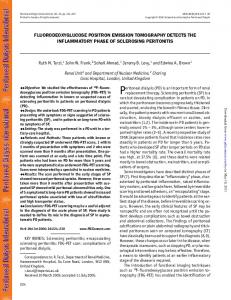
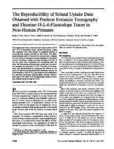
Modified Dunn’s Index (Average Linkage) This measure TAC data for all of the cluster measures discussed in the is based on the set distance function (2) [7]. substituted in previous section [17]. The optimal number of clusters (12) yielding the modified Dunn’s Index corresponding to the Average Linkage distance. Modified Dunn’s Index (Complete Linkage) As the name suggests, this measure is based on the set distance function (1). It has been observed that when this measure is used in the Dunn’s Index, it may be affected by the noisy points in , , the dataset because it does not use all the points in Xj and Xk . However, it has been asserted [7] that complete linkage produces quite useful hierarchies in most applications and that it usually produces clusters that are tight and hyperspherical. , , Modified Dunn’s Index (Combined Average) This measure combines the averaging concept of DAL with the idea of Fig. 2. Average Spread Comparison Plots for slices 4, 16 and 27 of computing the distance between the TACs within a cluster subjects #3246 and #4248 (Integrals) to the mean TAC of a different cluster. The set distance function is represented as p03246dy1 , Slice Number:4
p03246dy1 , Slice Number:16
0.08
0.09
0.07 0.06
0.08
0.04
0.04
0.03
0.03
4
4.5 5 5.5 6 Number of Clustergroups
6.5
7
3
0.03
0.06
0.04
0.03
0.03
6.5
7
3
Mean TAC for HAL2, Subject:3246, Slice 16
0.02
4.5 5 5.5 6 Number of Clustergroups
6.5
HCL HCL [1] HCL [2] HAL HAL[1] HAL [2] K Means
−0.005 0
10
20 30 Time in Minutes
40
50
,
−0.005 0
Separation 4
4.5 5 5.5 6 Number of Clustergroups
6.5
,
7
0.4
0.3
0.3
0.25
6.5
,
7
0.2 3
3.5
4
4.5 5 5.5 6 Number of Clustergroups
6.5
7
6.5
,
7
HCL HCL [1] HCL [2] HAL HAL[1] HAL [2] K Means
0.35
0.25
4.5 5 5.5 6 Number of Clustergroups
4.5 5 5.5 6 Number of Clustergroups
0.4
0.35
0.3
4
4
0.45
0.25
3.5
3.5
0.5
Separation
0.4
0.2 3
HCL HCL [1] HCL [2] HAL HAL[1] HAL [2] K Means
p03246dy1 , Slice Number:27
0.45
0.35
7
0.35
0.2 3
HCL HCL [1] HCL [2] HAL HAL[1] HAL [2] K Means
0.5
0.2 3
3.5
4
4.5 5 5.5 6 Number of Clustergroups
6.5
7
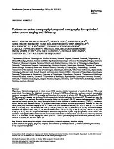
obtained from the different clustering algorithms could be observed from the peaks in the plots for the inter-intra cluster validity measures such as those shown in Figure 4 and Figure 5. p03246dy1 , Slice Number:4
p03246dy1 , Slice Number:16
0.6
0.62
0.58 0.56
0.6
0.54 0.52
4
4.5 5 5.5 6 Number of Clustergroups
6.5
,
7
0.62
0.56
0.52
3
HCL HCL [1] HCL [2] HAL HAL[1] HAL [2] K Means
0.64
0.58
0.54
3.5
p04248dy1 , Slice Number:27 HCL HCL [1] HCL [2] HAL HAL[1] HAL [2] K Means
0.64
Total Silhouette
0.62
Total Silhouette
HCL HCL [1] HCL [2] HAL HAL[1] HAL [2] K Means
0.64
0.6 0.58 0.56 0.54 0.52
3.5
p04248dy1 , Slice Number:4
4
4.5 5 5.5 6 Number of Clustergroups
6.5
,
7
3
3.5
p04248dy1 , Slice Number:16 HCL HCL [1] HCL [2] HAL HAL[1] HAL [2] K Means
0.62
0.01 0.005
0
3.5
6.5
0.4
0.35
0.2 3
4.5 5 5.5 6 Number of Clustergroups
0.5
p04248dy1 , Slice Number:16
0.45
Total Silhouette
0.01
0
,
7
4
0.45
0.3
4
3.5
p04248dy1 , Slice Number:27 HCL HCL [1] HCL [2] HAL HAL[1] HAL [2] K Means
0.25
0.5
0.02
0.015
0.005
3
0.3
Mean TAC for K−Means, Subject:3246, Slice 16
Intensity
Intensity
Intensity
0.01
7
0.25
0.64
0.005
6.5
4
4.5 5 5.5 6 Number of Clustergroups
6.5
7
p03246dy1 , Slice Number:27
0.025
0.015 0.015
4.5 5 5.5 6 Number of Clustergroups
0.6
HCL HCL [1] HCL [2] HAL HAL[1] HAL [2] K Means
0.64 0.62
0.58 0.56
0.6
0.62
0.58 0.56
0.54
0.54
0.52
0.52
HCL HCL [1] HCL [2] HAL HAL[1] HAL [2] K Means
0.64
Total Silhouette
0.025
0.02
4
0.4
Total Silhouette
0.025
0.06
0.3
3
0.03
0.07
0.03
p04248dy1 , Slice Number:4
Total Silhouette
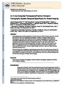
The mean tissue TACs were computed for the clusters obtained using the different clustering algorithms. A pairwise comparison of the mean TACs revealed high degree of similarity between the different algorithms. It was observed that the order of the clusters that need to be compared may vary depending upon the method. For example, Figure 1 reveals that the order of clusters produced using K-means is different from those using hierarchical methods. Hence, it is important to correctly order the groups prior to any comparisons across clustering methods. The Mean TAC for HCL1, Subject:3246, Slice 16
0.08
0.25
3.5
HCL HCL [1] HCL [2] HAL HAL[1] HAL [2] K Means
0.04
3.5
0.5
Separation
Separation
0.4
7
0.05
0.45
0.35
6.5
0.1
p03246dy1 , Slice Number:16 HCL HCL [1] HCL [2] HAL HAL[1] HAL [2] K Means
4.5 5 5.5 6 Number of Clustergroups
0.09
0.06
0.04
4
p03246dy1 , Slice Number:27
0.07
0.05
0.2 3
3.5
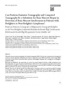
Fig. 3. Separation Comparison Plots for slices 4, 16 and 27 of subjects #3246 and #4248 (TACs)
V. Results
0.03
3
0.11
0.08
0.05
Separation
(13) The above inter-intra cluster measures are useful in finding an optimal number of clusters. A global maximum value of these indices for a set of different number of cluster groupings help in determining the optimal number of clusters. It is also deduced that the inter-cluster separation measures are more important in assessing cluster reliability than the actual individual cluster characteristics.
7
0.1
0.07
0.45
Separation
y∈Xk
6.5
HCL HCL [1] HCL [2] HAL HAL[1] HAL [2] K Means
p03246dy1 , Slice Number:4
x∈Xj
4.5 5 5.5 6 Number of Clustergroups
Average Spread
Average Spread
0.08
0.5
X X 1 d(x, µk ) + d(y, µj )} { DCAL (Xj , Xk ) = nj + nk
4
0.09
Average Spread
0.1
0.09
4.5 5 5.5 6 Number of Clustergroups
0.06
0.04
3.5
0.11
HCL HCL [1] HCL [2] HAL HAL[1] HAL [2] K Means
4
0.07
p04248dy1 , Slice Number:16
0.11
3.5
0.08
0.05
p04248dy1 , Slice Number:4
3
0.09
0.06 0.05
HCL HCL [1] HCL [2] HAL HAL[1] HAL [2] K Means
0.1
0.07
0.05
3.5
0.11
HCL HCL [1] HCL [2] HAL HAL[1] HAL [2] K Means
0.1
Average Spread
Average Spread
0.09
3
p04248dy1 , Slice Number:27
0.11
HCL HCL [1] HCL [2] HAL HAL[1] HAL [2] K Means
0.1
Average Spread
0.11
0.6 0.58 0.56 0.54
0
10
20 30 Time in Minutes
40
50
,
−0.005 0
10
20 30 Time in Minutes
40
50
Fig. 1. Mean TACs for subject #3246, slice= 16, Number of Clusters= 5 using HCL1, HAL2 and K-Means algorithms
quantitative results for the various cluster measures were plotted for both the integral and TAC data. Figure 2 and Figure 3 represent the plots obtained for average spread (intra-cluster) and separation (inter-cluster) across different slices and subjects. The results indicate close similarity in the homogeneity of the clusters obtained using different algorithms. Similar plots were plotted using integral and
3
3.5
4
4.5 5 5.5 6 Number of Clustergroups
6.5
7
,
3
0.52
3.5
4
4.5 5 5.5 6 Number of Clustergroups
6.5
7
,
3
3.5
4
4.5 5 5.5 6 Number of Clustergroups
6.5
7
Fig. 4. Silhouette Comparison Plots for slices 4, 16 and 27 of subjects #3246 and #4248 (Integrals)
VI. Conclusions We hope that this paper provides the basis for a validation strategy for comparing different clustering methods that can be used in the context of dynamic human PET data. No other studies of clustering for dynamic PET data, to the best of our knowledge, appear to have considered the
p03246dy1 , Slice Number:4
p03246dy1 , Slice Number:16
0.55 Mixed Linkage Ratio
0.5
0.45
0.4
0.35
0.3 3
0.5
0.4
0.35
3.5
4
4.5 5 5.5 6 Number of Clustergroups
6.5
,
7
HCL HCL [1] HCL [2] HAL HAL[1] HAL [2] K Means
3.5
Mixed Linkage Ratio
4
4.5 5 5.5 6 Number of Clustergroups
6.5
,
7
HCL HCL [1] HCL [2] HAL HAL[1] HAL [2] K Means
0.6
0.5
0.45
0.4
0.35
References 3.5
6.5
7
,
4.5 5 5.5 6 Number of Clustergroups
6.5
7
[1] HCL HCL [1] HCL [2] HAL HAL[1] HAL [2] K Means
0.6
0.5
0.45
0.4
0.3 3
4
0.55
0.35
4.5 5 5.5 6 Number of Clustergroups
0.3 3
p03246dy1 , Slice Number:27
0.55 Mixed Linkage Ratio
0.6
4
0.4
p04248dy1 , Slice Number:16
0.55
3.5
0.5
0.45
In future work we will also assess the robustness of calculation of parametric values from the cluster curves as another method of cluster comparison.
0.35
p04248dy1 , Slice Number:4
0.3 3
0.55
0.45
0.3 3
HCL HCL [1] HCL [2] HAL HAL[1] HAL [2] K Means
0.6
Mixed Linkage Ratio
Mixed Linkage Ratio
0.55
p04248dy1 , Slice Number:27 HCL HCL [1] HCL [2] HAL HAL[1] HAL [2] K Means
0.6
Mixed Linkage Ratio
HCL HCL [1] HCL [2] HAL HAL[1] HAL [2] K Means
0.6
0.5
[2]
0.45
0.4
0.35
3.5
4
4.5 5 5.5 6 Number of Clustergroups
6.5
7
,
0.3 3
[3] 3.5
4
4.5 5 5.5 6 Number of Clustergroups
6.5
7
Fig. 5. Combined Average Ratio Comparison Plots for slices 4, 16 and 27 of subjects #3246 and #4248 (TACs) [4]
use of clustering measures to identify the optimal number of clusters in the data. This may be a potential benefit of the results of the work since more insight into this information could lead to more efficient segmentation of the images thereby leading to better quantification of voxel level parameters. Another potential benefit is that we can compare the results obtained from the faster variants of hierarchical clustering to their more traditional counterparts. With the help of standard intra-cluster and inter-cluster measures that have been described in prior studies, we were able to quantify the cluster results with unique scalar values for each method as a whole. The results indicate that the cluster results obtained from the less expensive hierarchical algorithms are comparable to those obtained from the traditional hierarchical algorithms that are more expensive. K-means was observed to produce meaningful results in most instances. It is significantly faster than the hierarchical algorithms but the average dissimilarity within the clusters was observed to be relatively high and the separation between clusters was also found to be relatively low compared to the clusters obtained from hierarchical methods. Overall, we determined the pre-processed PET data to be quite amenable to the traditional clustering strategies and from a visual perspective, the clusters were quite meaningful. This is mainly attributed to the appropriate weighting scheme that was employed to determine the dissimilarity between different pixels/voxels. Four different intra-inter cluster measures as described in Section IV were used to assess the overall goodness and optimality of the clusters. All of them, by definition, would indicate an optimal number of clusters based upon the maximum value of the measure over different number of clusters. The consensus value ranges between 3 and 5 for different slices and different subjects. The results greatly varied within different slices of the same subject and between different subjects. The possibility that these measures may return sub-optimal clusters to be the most optimal cannot be fully ruled out. We are trying to get help of domain experts in determining an optimal number of clusters for a given slice based upon visual interpretation. With the help of this knowledge, we can determine the number of instances when a particular measure conforms with or differs from the calls made by the domain experts.
[5] [6] [7] [8] [9] [10] [11]
[12]
[13] [14] [15]
[16] [17]
[18]
P. D. Acton, L. S. Pilowsky, H. F. Kung, and P. J. Ell. Automatic segmentation of dynamic neuroreceptor single-photon emission tomography images using fuzzy clustering. Eur. J. Nucl. Med., 26(6):582 – 590, 1999. J. C. Bezdek and N. R. Pal. Some new indexes of cluster validity. Part B: Cybernetics, 28(3):301 – 315, 1999. K. Chen, D. Bandy, E. Reiman, S.-C. Huang, M. Lawson, D. Feng, L.-S. Yun, and A. Palant. Noninvasive quantification of the cerebral metabolic rate for glucose using positron emission tomography, 18 F-fluorodeoxyglucose, the Patlak method, and an image-derived input function. J. Cereb. Blood Flow Metab., 18:716–723, 1998. L.P. Clarke, R. P. Velthuizen, M. A. Camacho, J. J. Heine, M. Vaidyanathan, L. O. Hall, R. W. Thatcher, and M. L. Silbiger. MRI segmentation:methods and applications. Magn. Reson. Imag., 13(3):343–368, 1995. D. Dunn. Well separated clusters and optimal fuzzy partitions. J. Cybernet., 4:95–104, 1974. H. Guo, R. A. Renaut, K. Chen, and E. Reiman. Clustering huge data sets for parametric PET imaging. Biosystems, 71(12):81–92, 2003. A. K. Jain and R. C. Dubes. Algorithms for Clustering Data. Prentice Hall, 1988. A. K. Jain, M. N. Murty, and P. J. Flynn P.J. Data clustering: A review. ACM Computing Surveys, 31(3):264 – 323, 1999. L. Kaufman and P. Rousseeuw. Finding groups in Data : An introduction to Cluster Analysis. John Wiley and Sons, 1990. Y. Kimura, M. Senda, and N. Alpert. Fast formation of statistically reliable FDG parametric images based on clustering and principal components. Phys. Med. Biol., 47(3):455–468, 2002. M. Liptrot, K. H. Adams, L. Martiny, L. H. Pinborg, M. N. Lonsdale, N. V. Olsen, S. Holm, C. Svarer, and G. M. Knudsen. Cluster analysis in kinetic modelling of the brain: a noninvasive alternative to arterial sampling. Neuroimage, 21(2):483–493, 2004. J. McQueen. Some methods for classification and analysis of multivariate observations. Proceedings of the Fifth Berkeley Symposium on Mathematical Statistics and Probability, pages 281–297, 1967. G. A. F. Seber. Multivariate Observations. Wiley, 1984. R. R. Sokal and C. D.Michener. A statistical method for evaluating systematic relationships. University of Kansas Science Bulletin, 38:1409 – 1438, 1958. L. Sokoloff, M. Reivich, and C. Kennedy. The (14 c)deoxyglucose method for the measurement of local cerebral glucose utilization: theory, procedure and normal values in the conscious and anesthetized albino rat. J. Neurochem., 28:897–910, 1977. H. Spath. Cluster Dissection and Analysis: Theory, FORTRAN Programs, Examples. Halsted Press, 1985. Prasanna K Velamuru. Validation of clustering methods for pet data. Computational Biosciences Program Internship Report 05-02, Arizona State University, Tempe, AZ 85287-1804, 2005. Internship Report (No: 05-02). Y. Zhou. Model fitting with spatial constraint for parametric imaging in dynamic PET studies. PhD thesis, UCLA, Biomedical Physics, Advisor: Sung-Cheng Huang, 2000.