decentralised load-frequency control using an iterative linear matrix inequalities
algorithm. IEE Proceedings - Generation, Transmission and Distribution.
QUT Digital Repository: http;;//eprints.qut.edu.au
Bevrani, Hassan and Mitani, Yasunori and Tsuji, Kiiichiro (2004) Robust decentralised load-frequency control using an iterative linear matrix inequalities algorithm. IEE Proceedings - Generation, Transmission and Distribution 151(3):pp. 347-354.
© Copyright 2004 IEEE Personal use of this material is permitted. However, permission to reprint/republish this material for advertising or promotional purposes or for creating new collective works for resale or redistribution to servers or lists, or to reuse any copyrighted component of this work in other works must be obtained from the IEEE.
Robust decentralised load-frequency control using an iterative linear matrix inequalities algorithm H. Bevrani, Y. Mitani and K. Tsuji Abstract: The load-frequency control (LFC) problem has been one of the major subjects in electric power system design/operation and is becoming much more significant today in accordance with increasing size, changing structure and complexity of interconnected power systems. In practice LFC systems use simple proportional-integral (PI) controllers. However, since the PI controller parameters are usually tuned based on classical or trial-and-error approaches, they are incapable of obtaining good dynamical performance for a wide range of operating conditions and various load changes scenarios in a multi-area power system. For this problem, the decentralised LFC synthesis is formulated as an HN-control problem and is solved using an iterative linear matrix inequalities algorithm to design of robust PI controllers in the multi-area power systems. A three-area power system example with a wide range of load changes is given to illustrate the proposed approach. The resulting controllers are shown to minimise the effect of disturbances and maintain the robust performance.
List of symbols Dfi DPgt DPci DPti DPtie�i DPdi Mi Di Tgi Tti Tij Bi ai Ri
1
frequency deviation governor valve position governor load setpoint turbine power net tie-line power flow area load disturbance equivalent inertia constant equivalent damping coefficient governor time constant turbine time constant tie-line synchronising coefficient between areas i and j frequency bias area control error participation factor drooping characteristic
Introduction
Currently, the electric power industry is in transition from vertically integrated utilities (VIU) providing power at regulated rates to an industry that will incorporate competitive companies selling unbundled power at lower rates. In the new power system structure, load-frequency control (LFC) acquires a fundamental role to enable power exchanges and to provide better conditions for electricity trading. The common LFC objectives in the restructured power system, i.e. restoring the frequency and the net interchanges r IEE, 2004 IEE Proceedings online no. 20040493 doi:10.1049/ip-gtd:20040493 Paper first received 21st August 2003 and in revised form 26th February 2004 H. Bevrani and K. Tsuji are with the Department of Electrical Engineering, Osaka University, 2-1 Yamada-Oka, Suita, Osaka, Japan Y. Mitani is with the Department of Electrical Engineering, Kyushu Institute of Technology, Kyushu, Japan IEE Proc.-Gener. Transm. Distrib., Vol. 151, No. 3, May 2004
to their desired values for each control area remain [1]. That is why during the past decade several proposed LFC scenarios attempted to adapt well tested traditional LFC schemes to the changing environment of power system operation under deregulation [2–5]. In the new environment the overall power system can also be considered as a collection of control areas interconnected through high voltage transmission lines or tie-lines. Each control area consists of a number of generating companies (Gencos) and it is responsible for tracking its own load and performing the LFC task. There has been continuing interest in designing loadfrequency controllers with better performance to maintain the frequency and to keep tie-line power flows within prespecified values, using various decentralised robust and optimal control methods during the last two decades [6–13]. But most of them suggest complex state-feedback or highorder dynamic controllers, which are not practical for industrial practices. Furthermore, some authors have used the new and untested LFC frameworks, which may have some difficulties in being implemented in real-world power systems. Usually, the existing LFC systems in the practical power systems use the proportional-integral (PI) type controllers that are tuned online based on classical and trial-and-error approaches. Recently, some control methods have been applied to design the decentralised robust PI or low-order controllers to solve the LFC problem [14–17]. A PI control design method has been reported [14], which used a combination of HN control and genetic algorithm techniques for tuning the PI parameters. The sequential decentralised method based on m-synthesis and analysis has been used to obtain a set of low-order robust controllers [15]. The decentralised LFC method has been used with structured singular values [16]. The Kharitonov theorem and its results have been used to solve the same problem [17]. In this paper, the decentralised LFC problem is formulated as a standard HN control problem to obtain the PI controller via a static output feedback design. An iterative linear matrix inequalities (ILMI) algorithm is used to compute the PI parameters. The proposed strategy is applied to a three-control area example. The obtained 347
robust PI controllers, which are ideally practical for industry, are compared with the HN-based output dynamic feedback controllers (using the standard ILMIbased HN technique). Results show the controllers guarantee the robust performance for a wide range of operating conditions as well as full-dynamic HN controllers. 2
This Section gives a brief overview of HN-static output feedback controller design based on an ILMI approach. Consider a linear time invariant system G(s) with the following state-space realisation. x_ ¼Ax þ B1 w þ B2 u z ¼C1 x þ D12 u
ð1Þ
y ¼C2 x where x is the state variable vector, w is the disturbance and other external input vector, z is the controlled output vector and y is the measured output vector. The static output HN controller problem is to find a static output feedback u ¼ Ky, as shown in Fig. 1, such that the resulting closed-loop system is internally stable, and the HN norm from w to z is smaller than g, a specified positive number, i.e. jjTzw ðsÞjj1 og
ð2Þ
w
z G (s)
Closed-loop system via HN control
Theorem 1 It is assumed (A, B2, C2) is stabilisable and detectable. The matrix K is an HN controller, if and only if there exists a symmetric matrix X40 such that 2
ATcl X þ XAcl 4 BTcl X Ccl
XBcl �gI Dcl
3 T Ccl DTcl 5o0 �gI
0
3 B2 7 � 7 � 6 ¼ ½ C2 5; B ¼ 4 0 5; C D12 �gI=2 0 0
3
2
Ccl ¼ C1 þ D12 KC2 ;
Bcl ¼ B1 Dcl ¼ 0
The proof is given in [18, 19]. We can rewrite (3) as the following matrix inequality [20]: � þ ðXBK C � ÞT þ A � T X� þ XAo0 XBK C
0� ð5Þ
X X� ¼ 4 0 0
3 0 0 I 05 0 I
Hence, the static output feedback HN control problem is reduced to find X40 and K such that matrix inequality (4) holds. It is a generalised static output feedback stabilisation �; B � Þ which can be solved via �; C problem of the system ðA theorem 2, given in the Appendix (Section 9). A solution of the consequent nonconvex optimisation problem, introduced in theorem 2, cannot be directly achieved by using general LMI technique. On the other hand, the matrix inequality (22) points to an iterative approach to solve the matrix K and X, namely, if P is fixed, then it reduces to an LMI problem in the unknowns K and X. For this purpose, we introduce the following ILMI algorithm that is mainly based on the approach given in [21]. The key point is to formulate the HN problem via a generalised static output stabilisation feedback such that all eigenvalues of (A-BKC) shift towards the left half-plane through the reduction of a, a real number, to close to feasibility of (22). In summary, the HN-static output feedback controller design based on the ILMI approach for a given system consists of the following steps: �; B � Þ, according to (5). �; C Step 1 Compute the new system ðA Set i ¼ 1 and Dg ¼ Dg0. Let gi ¼ g0 a positive real number. Step 2 Select Q40, and solve X� from the following algebraic Riccati equation: ð6Þ
Set P1 ¼ X� . Step 3 Solve the following optimisation problem for X�i , Ki and ai. Minimise ai subject to the LMI constraints 2 T � X�i þ X�i A � � Pi B �B � T X�i � X�i B �B � T Pi A 6 �B � T Pi � ai X�i þPi B 4 � � T X�i þ Ki C B ð7Þ # T T � � X�i þ Ki C Þ ðB o0 �I
X�i ¼ X�iT 40 Acl ¼ A þ B2 KC2 ;
0
ð3Þ
where
348
B1 �gI=2
� � XBB � T X� þ X� A � T X� þ Q ¼ 0 A
y
K
Fig. 1
A 6 � ¼4 0 A C1
2
HN-static output feedback using ILMI
u
where 2
ð4Þ
ð8Þ
Denote a�i as the minimised value of ai. Step 4 If a�i � 0, go to step 8. Step 5 For i41 if a�i�1 � 0, Ki�1 is the desired HN controller and g� ¼ gi þ Dg indicates a lower bound such that the above system is HN stabilisable via static output feedback. Step 6 Solve the following optimisation problem for X�i and Ki. Minimise trace (X�i ) subject to the above LMI constraints IEE Proc.-Gener. Transm. Distrib., Vol. 151, No. 3, May 2004
(7) and (8) with ai ¼ a�i . Denote X�i� as the X�i that minimised trace (X�i ). � , then go to step 3. Step 7 Set i ¼ i+1 and Pi ¼ X�i�1 Step 8 Set gi ¼ gi � Dg, i ¼ i+1. Then do steps 2–4. The matrix inequalities (7) and (8) give a sufficient condition for the existence of the static output feedback controller. 3
Problem formulation and dynamical model
A large-scale power system consists of a number of interconnected control areas. Figure 2 shows the block diagram of control area-i, which includes n Gencos, from an N-control area power system. As is usual in the LFC design literature, three first-order transfer functions are used to model generator, turbine and power system (rotating mass and load) units. w1i and w2i show local load disturbance and area interface, respectively. The other parameters are described in the list of symbols at the front of this paper. Following a load disturbance within a control area, the frequency of that area experiences a transient change, the feedback mechanism comes into play and generates appropriate rise/lower signal to the participating Gencos
w2i ¼
According to Fig. 2, in each control area the ACE acts as the input signal of the PI controller which is used by the LFC system. Therefore we have Z ui ¼ DPci ¼ kPi ACEi þ kIi
α li
ui ¼ Ki yi
. . .
K (s)
α ni
+
Genco n −
+
1+sTtli rate limiter . . .
Wli
∆Ptli
∆Pgli 1
1 Rn
controller
ð14Þ
Finally, the described ILMI-based HN algorithm will be used to obtain the desired PI parameters. The main control framework to formulate the PI-based LFC via a static
1
governor . . .
ð13Þ
we can rewrite (12) as follows [14]: � � ACEi R ui ¼ ½kPi kIi � ACEi
1+sTgli
∆PCi
ACEi + +
−
+
ð12Þ
ACEi
In the next step, as shown in Fig. 3, the PI-based LFC design can be reduced to a static output feedback control problem. To change (12) to a simple static feedback control as
Genco 1
R1
ð11Þ
Tij Dfj
j¼1 j6¼i
1 Bi
N X
+
−
1
−
Di +sMi
turbine . . .
∆fi
power system N
∆Pgni
Σ Tij
∆Ptni
1
1
1+sTgni
1+sTtni
j=l j≠i
+ 2π/s ∆Ptie −i
− W2i
Fig. 2
General control area
according to their participation factors (aji) to make generation follow the load. In the steady state, the generation is matched with the load, driving the tie-line power and frequency deviations to zero. The balance between connected control areas is achieved by detecting the frequency and tie-line power deviations to generate the area control error (ACE) signal which is, inturn, utilised in the PI control strategy as shown in Fig. 2. The ACE for each control area can be expressed as a linear combination of tie-line power change and frequency deviation. ACEi ¼ Bi Dfi þ DPtie�i
PI control design problem
Ki (s) = kPi +
Ki = [ kPi k li ]
ð9Þ
IEE Proc.-Gener. Transm. Distrib., Vol. 151, No. 3, May 2004
ð10Þ
S
static output feedback control problem
It can be shown that considering w1i and w2i as two input disturbance channels is useful to decentralised LFC design [22]. These signals can be defined as follows: w1i ¼ DPdi
k li
ILMI-based H∞ solution
Fig. 3
Problem formulation 349
2
�1i ∆fi
w1i
Ai11
�2i ACEi zi ∫
wi w2i
Gi (s)
�3i ui
2
ACEi
∫ ACEi
ui
Ai31
�1=ðTgni Rni Þ 2
B1i1
zi ¼C1i xi þ D12i ui yi ¼C2i xi
ð15Þ
xgi �
xti
ACEi
xti ¼ ½ DPt1i
DPt2i
� � � DPtni �
xgi ¼ ½ DPg1i
DPg2i
� � � DPgni �
R
yi ¼ ½ ACEi zTi ¼ ½ Z1i Dfi
ACEi � ;
ð16Þ
ð17Þ
Z3i ui �
ð18Þ
w2i �
ð19Þ
and 2
Ai11
Ai12
6 Ai ¼4 Ai21 Ai22 Ai31 Ai32 2 3 B2i1 6 7 B2i ¼4 B2i2 5 B2i3
Ai13
3
2
2 D12i
0
03�n 3
Z1i
6 03�n �; c1i ¼ 4 0 0
3
0
0
3
7 0 Z2i 5 0 0
C2i ¼ ½ c2i
���
To illustrate the effectiveness of proposed control strategy, a three-control area power system, shown in Fig. 5, is considered as a test system. It is assumed that each control area includes three Gencos. The total generation of each Genco in MW is given in Table 1. The power system parameters are considered to be the same as in [14]. For the sake of comparison, in addition to the proposed control strategy to obtain the robust PI controller, a robust HN dynamic output feedback controller using the LMI control toolbox is designed for each control area. Specifically, based on a general LMI, first the control design is reduced to a LMI formulation [14], and then the HN control problem is solved using the function hinflmi, provided by the MATLAB LMI control toolbox [23]. This function gives an optimal HN controller through the minimising the guaranteed robust performance index (2) subject to the constraint given by the matrix inequality (3) and returns the controller K(s) with optimal robust performance index. The resulted controllers using the hinflmi function are of dynamic type and have the following state-space form, whose orders are the same as size of plant model (9th order in the present paper): ui ¼Cki xki þ Dki yi
02�n
Bi 02�n �; c2i ¼ 0
1 0
0 1
�
ani =Tgni �
Application to a 3-control area power system
x_ ki ¼Aki xki þ Bki yi
6 7 ¼4 0 5 Z3i �
350
B1i1
7 6 7 Ai23 5; B1i ¼ 4 B1i2 5 Ai33 B1i3
2 C1i ¼½ c1i
3 0 �2p 5; B1i2 ¼ B1i3 ¼ 0n�2 0
Similar to [14], three constant weighting coefficients are considered for controlled output signals. Z1i, Z2i and Z3i must be chosen by the designer to obtain the desired performance. 4
ui ¼ DPCi
R Z2i ACEi
wTi ¼ ½ w1i
�1=Mi ¼4 0 0
0
3 0 .. 7 7 . 5; 0
¼ 03�n ; Ai32 ¼ 0n�n
B2i1 ¼03�1 ; B2i2 ¼ 0n�1 BT2i3 ¼½ a1i =Tg1i a2i =Tg2i
where
T
1 0 3 1=Mi 7 0 5 0 3�n
�1=ðTg1i R1i Þ 0 6 .. .. ¼6 . . 4
Ai13 ¼ATi21
x_ i ¼Ai xi þ B1i wi þ B2i ui
DPtie�i
3
7 07 7 7 5
0
2
output HN controller design problem, for a given control area, is shown in Fig. 4. Gi(s) denotes the dynamical model corresponds to control area i shown in Fig. 2. According to (1), the state space model for each control area i can be obtained as
xTi ¼ ½ Dfi
��� ���
0
Ai22 ¼ � Ai23 ¼ diag½ �1=Tt1i �1=Tt2i � � � �1=Ttni � Ai33 ¼diag½ �1=Tg1i �1=Tg2i � � � �1=Tgni �
Proposed control framework
R
�1=Mi
Bi 1=Mi � � �
6 Ai12 ¼4 0 0
yi
Ki = [ kPi kIi ]
Fig. 4
�Di =Mi 6 P N 6 2p T 6 ¼6 j¼1 ij 4 j6¼i
ð20Þ
At the next step, according to the synthesis methodology described in Section 2 and summarised in Fig. 6, a set of three decentralised robust PI controllers are designed. As has already been mentioned, this control strategy is fully suitable for LFC applications which usually employ the PI IEE Proc.-Gener. Transm. Distrib., Vol. 151, No. 3, May 2004
Genco 2
Genco 3
Genco 4
Genco 5
Genco 6
load 2
Genco 1
area 2
load 1
area 1
Genco 7
Fig. 5
Genco 8
Genco 9
load 3
area 3
Three-control area power system
Table 1: Total generation of Gencos Genco
1
2
3
4
5
6
7
8
9
Rate, MW
1000
1200
1000
1100
900
1200
900
1000
1100
(MVAbase : 1000 MW)
Table 2: Control parameters (ILMI design) set initial values and compute (A, B, C )
Parameter
Area 1
Area 2
Area 3
a*
�0.3285
�0.2472
�0.3864
kPi
0.0371
0.0465
0.0380
solve X from (6),
kIi
�0.2339
�0.2672
�0.3092
set Pi = X
Zji
Z1i ¼ 0.5
Z2i ¼ 1
Z3i ¼ 500
(A, B, C) Q>0
Pi γi = γi −∆γ
minimise ai subject to (7 and 8)
i=i+1
i=i+1
Ki ai* , Xi
yes
Pi = Xi*−1
a*i ≤ 0
no
minimise trace (X) subject to (7 and 8)
i >1 no
(i =1)
yes
K = Ki −1 a* = a*i −1 γ * = γi −1
Fig. 6
LFC design algorithm using ILMI
IEE Proc.-Gener. Transm. Distrib., Vol. 151, No. 3, May 2004
control, while most other robust and optimal control designs (such as the LMI approach) yield complex controllers whose size can be larger than real-world LFC systems. Using the ILMI approach, the controllers are obtained following several iterations. The control parameters are shown in Table 2. A set of suitable values for constant weights [Z1i, Z2i, Z3i] can be chosen as [0.5, 1, 500], respectively. An important issue with regard to selection of these weights is the degree to which they can guarantee the satisfaction of design performance objectives. The selection of these weights entails a trade-off among several performance requirements. The coefficients Z1i and Z2i at controlled outputs set the performance goals, e.g. tracking the load variation and disturbance attenuation. Z3i sets a limit on the allowed control signal to penalise fast change and large overshoot in the governor load set-point signal. The recent objective is very important to realise the designed controller in the real-world power systems. The large coefficient ‘500’ for Z3i results in a smooth control action signal with reasonable changes in amplitude. It is notable that the robust performance index given by the standard HN control design (2) can be used as a valid 351
0.1
g�3
(Area 2)
(Area 3)
HN
9th order
500.0103
500.0045
500.0065
ILMI
PI
500.0183
500.0140
500.0105
tool to analyse robustness of the closed-loop system for the proposed control design. The resulting robust performance indices (g*) of both synthesis methods are too close to each other and are shown in Table 3. It shows that although the proposed ILMI approach gives a set of much simpler controllers (PI) than the robust HN design, they also give a robust performance like the dynamic HN controllers.
∆f 2, Hz ∆Pc 2, p.u.
To demonstrate the effectiveness of the proposed control design, some simulations were carried out. In these simulations, the proposed controllers were applied to the three-control area power system described in Fig. 5. In this Section, the performance of the closed-loop system using the robust PI controllers compared to the designed dynamic HN controllers will be tested for the various possible load disturbances. Case 1: As the first test case, the following large load disturbances (step increase in demand) are applied to three areas:
Conclusions
A new method for robust decentralised LFC design using an iterative LMI approach has been proposed for a largescale power system. The design strategy includes enough flexibility to set the desired level of performance and gives a set of simple PI controllers via the HN static output control design, which is commonly used in real-world power systems. The proposed method was applied to a three-control area power system and was tested with different load change scenarios. The results were compared with 352
10
15
20
25
0
5
10
15
20
25
0
5
10
15
20
25
0
0.1 0 −0.1
0.1 0 0
5
10
15
20
25
0
5
10
15
20
25
0
5
10
15
20
25
0.1 0 −0.1
0.1 0 −0.1
time, s b
∆f 3, Hz
0.1
DPd1 ¼ 100 MW; DPd2 ¼ 80 MW; DPd3 ¼ 50 MW
6
5
−0.1
−0.1
Simulation results
0
ACE3, p.u.
−0.1
∆Pc 3, p.u.
The frequency deviation (Df ), area control error (ACE) and control action (DPc) signals of the closed-loop system are shown in Fig. 7. Using the proposed method (ILMI), the area control error and frequency deviation of all areas are quickly driven back to zero as well as dynamic HN control (LMI). Case 2: Consider larger demands by areas 2 and 3, i.e. DPd1 ¼ 100 MW, DPd2 ¼ 100 MW, DPd3 ¼ 100 MW. The closed-loop responses for each control area are shown in Fig. 8. Case 3: As another severe condition, assume a bounded random load change, shown in Fig. 9, is applied to each control area, where �50 MWrDPdr50 MW. The purpose of this scenario is to test the robustness of the proposed controllers against random large load disturbances. The control area responses are shown in Fig. 10. This figure demonstrates that the designed controllers track the load fluctuations effectively. The simulation results show that the proposed PI controllers perform as robustly as the robust dynamic HN controllers (with complex structures) for a wide range of load disturbances.
0
0.1
time, s a
ACE2, p.u.
5
0 −0.1
ACE1, p.u.
(Area 1)
g�2
∆Pc 1, p.u.
Control design Control structure g�1
∆f 1, Hz
Table 3: Robust performance index
0
5
10
15
20
25
0
5
10
15
20
25
0
5
10
15
20
25
0.1 0 −0.1 0.1 0 −0.1
time, s c
Fig. 7
System response in case 1
F ILMI - - - - HN a Area 1 b Area 2 c Area 3
the results of applied dynamic HN output controllers. Simulation results demonstrated the effectiveness of the methodology. It was shown that the designed controllers can guarantee the robust performance, such as precise reference frequency tracking and disturbance attenuation under a wide range of area-load disturbances.
7
Acknowledgments
The authors are grateful to Dr. Y. Y. Cao from the University of Virginia, USA, Prof. M. Ikeda from Osaka University, Japan and Dr. D. Rerkpreedapong from Kasetsart University, Thailand for their kind discussions. IEE Proc.-Gener. Transm. Distrib., Vol. 151, No. 3, May 2004
0.1 ∆f 1, Hz
∆f 1, Hz
0.1 0 −0.1 5
10
15
20
−0.1
25
0.1
ACE1, p.u.
ACE1, p.u.
0 0 −0.1
∆Pc 1, p.u.
0
5
10
15
20
∆Pc 1, p.u.
0 0
5
10
15
20
0
10
20
30
40
50
60
70
80
0
10
20
30
40
50
60
70
80
0
10
20
30
40 50 time, s a
60
70
80
0
10
20
30
40
50
60
70
80
0
10
20
30
40
50
60
70
80
0
10
20
30
40 50 time, s b
60
70
80
10
20
30
40
50
60
70
80
10
20
30
40
50
60
70
80
10
20
30
40 50 time, s c
60
70
80
0.1 0 −0.1
25
0.1
−0.1
0
25
0.1 0 −0.1
time, s a
0.1
−0.1 5
10
15
20
25
0
0.1
−0.1
0
0.1
ACE2, p.u.
ACE2, p.u.
0
−0.1 0
∆Pc 2, p.u.
∆f 2, Hz
0
5
10
15
20
25
0
0.1
−0.1
0
0.1
−0.1
0
5
10
15
20
∆Pc 2, p.u.
∆f 2, Hz
0.1
25
time, s b
0 −0.1
0
0.1 5
10
15
20
25
0.1 0 −0.1
∆Pc 3, p.u.
0
5
10
15
20
ACE3, p.u.
ACE3, p.u.
0
∆f 3, Hz
−0.1
25
0.1 0 −0.1 0
5
10
15
20
∆Pc 3, p.u.
∆f 3, Hz
0.1
25
time, s c
Fig. 8
0 −0.1 0 0.1 0 −0.1 0 0.1 0 −0.1 0
System response in case 2
a Area 1 b Area 2 c Area 3 F ILMI - - - - HN
Fig. 10
System response in case 3
a Area 1 b Area 2 c Area 3 F ILMI - - - - HN
0.10 0.08 0.06
∆Pd, p.u.
0.04
8
0.02 0 −0.02 −0.04 −0.06 −0.08 −0.10
Fig. 9
0
10
20
30
40 50 time, s
60
70
Random load demand signal
IEE Proc.-Gener. Transm. Distrib., Vol. 151, No. 3, May 2004
80
References
1 Jaleeli, N., Van Slyck, L.S., Ewart, D.N., Fink, L.H., and Hoffmann, A.G.: ‘Understanding automatic generation control’, IEEE Trans. Power Syst., 1992, 3, (7), pp. 1106–1122 2 Kumar, J., Hoe, N.K., and Sheble, G.B.: ‘AGC simulator for pricebased operation, Part 1: A model’, IEEE Trans. Power Syst., 1997, 2, (12), pp. 527–532 3 Donde, V., Pai, A., and Hiskens, I.A.: ‘Simulation and optimisation in a AGC system after deregulation’, IEEE Trans. Power Syst., 2001, 3, (16), pp. 481–489 4 Bevrani, H., Mitani, Y., and Tsuji, K.: ‘On robust load-frequency regulation in a restructured power system’, Trans. Inst. Electr. Eng. Jpn., 2004, 124-B, (2), pp. 190–198 353
5 Delfino, B., Fornari, F., and Massucco, S.: ‘Load-frequency control and inadvertent interchange evaluation in restructured power systems’, IEE Proc., Gener. Transm. Distrib., 2002, 5, (149), pp. 607–614 6 Hiyama, T.: ‘Design of decentralised load-frequency regulators for interconnected power systems’, IEE Proc. C Gener. Transm. Distrib., 1982, 129, pp. 17–23 7 Feliachi, A.: ‘Optimal decentralized load frequency control’, IEEE Trans. Power Syst., 1987, 2, pp. 379–384 8 Liaw, C.M., and Chao, K.H.: ‘On the design of an optimal automatic generation controller for interconnected power systems’, Int. J. Control, 1993, 58, pp. 113–127 9 Wang, Y., Zhou, R., and Wen, C.: ‘Robust load-frequency controller design for power systems’, IEE Proc. C Gener. Transm. Distrib., 1993, 140, (1), pp. 11–16 10 Lim, K.Y., Wang, Y., and Zhou, R.: ‘Robust decentralised loadfrequency control of multi-area power systems’, IEE Proc., Gener. Transm. Distrib., 1996, 5, (143), pp. 377–386 11 Ishi, T., Shirai, G., and Fujita, G.: ‘Decentralized load frequency based on H-inf control’, Electr. Eng. Jpn, 2001, 3, (136), pp. 28–38 12 Kazemi, M.H., Karrari, M., and Menhaj, M.B.: ‘Decentralized robust adaptive-output feedback controller for power system load frequency control’, Electr. Eng. J, 2002, 84, pp. 75–83 13 El-Sherbiny, M.K., El-Saady, G., and Yousef, A.M.: ‘Efficient fuzzy logic load-frequency controller’, Energy Convers. Manage., 2002, 43, pp. 1853–1863 14 Rerkpreedapong, D., Hasanovic, A., and Feliachi, A.: ‘Robust load frequency control using genetic algorithms and linear matrix inequalities’, IEEE Trans. Power Syst., 2003, 2, (18), pp. 855–861 15 Bevrani, H., Mitani, Y., and Tsuji, K.: ‘Sequential design of decentralized load-frequency controllers using m-synthesis and analysis’, Energy Convers. Manage., 2004, 45, (6), pp. 865–881 16 Yang, T.C., Cimen, H., and Zhu, Q.M.: ‘Decentralised load frequency controller design based on structured singular values’, IEE Proc., Gener. Transm. Distrib., 1998, 145, (1), pp. 7–14 17 Bevrani, H.: ‘Application of Kharitonov’s theorem and its results in load-frequency control design’, Res. Sci. J. Electr. (BARGH), 1998, 24, pp. 82–95 18 Skelton, R.E., Stoustrup, J., and Iwasaki, T.: ‘The HN control problem using static output feedback’, Int. J. Robust Nonlinear Control, 1994, 4, pp. 449–455 19 Gahinet, P., and Apkarian, P.: ‘A linear matrix inequality approach to HN control’, Int. J. Robust Nonlinear Control, 1994, 4, pp. 421–448 20 Cao, Y.Y., Sun, Y.X., and Mao, W.J.: ‘Output feedback decentralized stabilization: ILMI approach’, Syst. Control Lett., 1998, 35, pp. 183– 194
354
21 Cao, Y.Y., Sun, Y.X., and Mao, W.J.: ‘Static output feedback stabilization: an ILMI approach’, Automatica, 1998, 12, (34), pp. 1641–1645 22 Bevrani, H., Mitani, Y., and Tsuji, K.: ‘Robust load-frequency regulation in a new distributed generation environment’, IEEE-PES General Meeting (CD record), Toronto, Canada, July 2003 23 Gahinet, P., Nemirovski, A., Laub, A.J., and Chilali, M.: ‘LMI Control Toolbox’, (The MathWorks, Inc, Natick, USA 1995) 24 Cao, Y.Y., and Sun, Y.X.: ‘Static output feedback simultaneous stabilization: ILMI approach’, Int. J. Control, 1998, 5, (70), pp. 803– 8144
9 Appendix Theorem 2 The system (A, B, C) that may also be identified by the following representation: x_ ¼Ax þ Bu y ¼Cx
ð21Þ
is stabilisable via static output feedback if and only if there exist P40, X40 and K satisfying the following quadratic matrix inequality: 2 3 AT X þ XA � PBBT X ðBT X þ KCÞT 4 �XBBT P þ PBBT P 5o0 ð22Þ T B X þ KC �I Proof According to the Schur complement, the quadratic matrix inequality (22) is equivalent to the following matrix inequality: AT X þ XA � PBBT X � XBBT P þ PBBT P þ ðBT X þ KCÞT ðBT X þ KCÞo0
ð23Þ
For this new inequality notation (23), the sufficiency and necessity of the theorem are already proven [24].
IEE Proc.-Gener. Transm. Distrib., Vol. 151, No. 3, May 2004