Parul Pandey, Mehdi Rahmati, Dario Pompili, and Waheed U. Bajwa. Department of Electrical and Computer Engineering. Rutgers UniversityâNew Brunswick, ...
Robust Distributed Dictionary Learning for In-network Image Compression Parul Pandey, Mehdi Rahmati, Dario Pompili, and Waheed U. Bajwa Department of Electrical and Computer Engineering Rutgers University–New Brunswick, NJ 08854, USA {parul.pandey, mehdi.rahmati, pompili, waheed.bajwa}@rutgers.edu Abstract—Camera networks are resource-constrained distributed systems that communicate over (wireless) networks to make decisions collaboratively. For surveillance applications, these camera nodes take decisions about an object of interest within incoming videos by coordinating with neighboring nodes, which is a costly process in terms of both time and energy. Datacompression methods can bring significant energy savings in camera nodes while transmitting or storing data in the network. Signal representation using sparse approximations and overcomplete dictionaries have received considerable attention in recent years and have been shown to outperform traditional compression methods. However, distributed dictionary learning itself relies on consensus-building algorithms, which involve communicating with neighboring nodes until convergence is achieved. To this end, we design a novel protocol to enable energy-efficient and robust dictionary learning in distributed camera networks by leveraging the spatial correlation of collected multimedia data. We employ low-computational-complexity metrics to quantify the correlation across cameras nodes. We also present a feasibility study of the parameters of the network that impact the performance of distributed dictionary learning and consensus process in terms of accuracy of the algorithm and energy consumed by the camera nodes. The performance of the proposed approach is validated through extensive simulations using a network simulator and public datasets as well as via real-world experiments on a testbed of Raspberry Pi nodes. Index Terms—Dictionary Learning; Camera Networks; Distributed Consensus; Image Compression; Mobile Computing.
There has been some recent works focusing on smart distributed camera networks that combine video sensing, processing, and communication on a single embedded platform. These camera nodes analyze the object of interest online on incoming videos and take decisions by running computationallyintensive computer-vision algorithms for detection and tracking of object of interest [2]. This requires communication between the camera nodes that involves multiple transmissions of raw data, which is a costly process (in terms of time and energy) for the resource-constrained nodes and reduces the mission lifetime of the nodes. These limitations call for efficient image-compression methods for transmission and storing of data in the network. Signal representation using sparse approximations and overcomplete dictionaries [3] have received considerable attention in recent years in the area of image feature extraction, data compression, and bit-rate reduction [4], [5], [6] for both storage and transmission. The goal of dictionary learning is to learn an overcomplete dictionary D such that data samples, represented as a matrix Y , are well approximated by no more than T0 columns of D. Mathematically, the problem of dictionary learning can be expressed as � D, X = arg min kY − DXk2F s.t. ∀s, kxks ≤ T0 , (1) D,X
I. I NTRODUCTION Motivation: Cameras networks are real-time distributed systems that cover large spaces and communicate over (wireless) networks to make decisions collaboratively. These cameras refer to a system of physically distributed camera nodes that may or may not have overlapping fields of view [1] and that allow us to see a subject of interest from several angles, helping resolve the problem of occlusion faced by individual cameras. Camera networks have been used in surveillance applications where the videos by the cameras are sent to a centralized location and are analyzed offline by the lawenforcement agencies. Sending video data (generated throughout the time of operation at 30-60 fps) from a large number of cameras in a network to a central server is expensive (in terms of time and energy of camera nodes) and inherently unscalable. The combination of large numbers of nodes, security concerns, expectation of fast response times, and delay in communicating data to the central node pushes us away from server-based architectures.
where Y is the data available at a centralized location, X ∈ RK×S are the sparse coefficients of the data having no more than T0 � n nonzero coefficient per sample, and xs represents the sth column in X. Once a dictionary is learned, each node can learn a sparse approximation of the signal that can be used along with an image-compression technique to help save significant space when storing the data and energy when offloading data to a centralized location or to neighboring nodes. Consensus forms the communication primitive to be used between neighboring camera nodes for dictionary learning in a setting where the data is distributed such as in distributed camera networks [7], [8]. In particular, consensus is an iterative process where the camera nodes communicate with their neighbors for a fixed number of iterations or until convergence. This iterative communication introduces an additional overhead of energy consumption on nodes in the network. Our Vision: We focus on developing energy-efficient dictionary-learning techniques for distributed camera net-
(a)
(b)
(c)
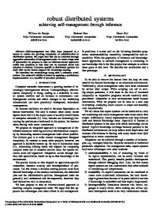
Fig. 1: Illustration of three different types of distributed camera networks where image compression using dictionary learning can bring potential benefits in saving battery capacity of camera nodes in the network. Each sensor node can serve as a Data Provider (DP) or a Resource Provider (RP). The RP nodes have sophisticated computational capabilities and higher battery capacity than DP nodes. (a) Mars exploration with Curiosity rover [9]; (b) Underwater environment covered with a network of Autonomous Underwater Vehicles (AUVs). AUVs serving as DP continuously capture raw data, while RPs—such as Mesobot and Sentry [10]—can create bathymetric maps and perform sidescan of the seafloor by taking and processing images in deep sea and oceans; (c) Deployment of multiview distributed cameras in a smart home application.
works. We consider a distributed camera network where the camera nodes have heterogeneous capabilities in terms of battery capacity and processor capabilities. We divide these camera nodes into two categories, namely, Data Provider (DP) and Resource Provider (RP). The DP nodes are dumb nodes in the sense that they are severely resource constrained and have limited computational capabilities. The RPs, on the other hand, have sophisticated computational capabilities and higher battery capacity than DP nodes. Figure 1 shows examples of various futuristic applications of the proposed distributed solution in harsh environments—such as on Mars and in underwater environments—as well as for consumer applications— such as in smart home cameras. Our Approach: We design a protocol to identify the camera nodes in the network with spatial correlated data by using only local knowledge of the network available to the camera nodes. We use computationally cheap metrics to quantify the correlation of data among camera nodes. We also present a feasibility study of the different parameters of the distributed dictionary learning algorithm and their impact on the accuracy of the algorithm and residual energy of the nodes in the network. Distributed dictionary learning can be used to enable a variety of applications in a distributed camera network such as background modeling and object classification [8], [11]; in this paper, we focus on in-network image compression. Contribution: The following are our main contributions. • We present via simulations the scalability of consensus in a wireless distributed computing infrastructure by varying the wireless network environment variables (i.e., density, connectivity, and number of consensus iterations). • We develop a protocol to enable energy-efficient, robust consensus process on resource-constrained camera nodes by identifying the network nodes with correlated data. • We quantify the trade-off in energy savings and loss in accuracy achieved for in-network image compression by implementing our protocol on a testbed of Rasberry Pi nodes. Paper Outline: The remainder of this paper is organized as follows. In Sect. II, we study how different consensus
parameters impact the feasibility of convergence. In Sect. III, we present details of the design of our protocol that is proposed to bring energy savings to the distributed dictionary-learning algorithm executed in a camera network. In Sect. IV, we provide quantitative results that demonstrate the merits of our contributions. In Sect. V, we cover the work done in the area of distributed systems employing consensus and analyze the difference of these approaches from ours. Finally, in Sect. VI, we conclude our paper and outline future work. II. D ICTIONARY L EARNING AND C ONSENSUS IN A D ISTRIBUTED C AMERA N ETWORK In this section we first present different steps of the distributed dictionary learning algorithm. We then show the performance of consensus and distributed dictionary learning in terms of accuracy of the algorithms and energy consumed by the nodes to run these algorithms in a network. This section will help us motivate the need to save energy during the execution of a distributed dictionary learning algorithm. A. Dictionary Learning in a Distributed Camera Network Assume N camera nodes used for surveillance form an ad-hoc network and communicate over a wireless network. Any wireless communications technology such as Bluetooth, WiFi Direct, 802.11 ad-hoc mode, or Near-field Communication (NFC) can be used in this scenario without relying on any existing fixed infrastructure. Two camera nodes are considered neighbors when they are in the communication range of each other. Each node is capable of storing some local data, performing computations on it, and exchanging messages with its neighbors. Next, we assume each node i has a collection of local data, expressed as a matrix Yi ∈ Rn×Si , with Si representing the number of data samples at the ith node. In case of distributed camera networks, each camera node is taking images of a scene from a different angle, which form the data samples at the ith node. We can express all this n×S distributed data , PN into a single matrix Y = [Y1 · · · YN ] ∈ R where S = i=1 Si denotes the total number of data samples distributed across the N nodes.
Fig. 2: Workflow for distributed dictionary learning executed at each camera node in the network. Task 1, 2, and 3 are executed locally at each node; whereas Task 4, i.e., consensus, involves communication between nodes that are in communication range of each other.
We reiterate the dictionary problem here; assume that the data Y is available at a centralized location, the problem of learning an overcomplete dictionary D can be expressed as, � D, X = arg min kY − DXk2F s.t. ∀s, kxks ≤ T0 , (2) D,X
K×S
where X ∈ R are the sparse coefficients of the data having no more than T0 � n nonzero coefficient per sample, and xs represents the sth column in X. In a distributed setting, the goal of dictionary learning is to have individual nodes b i }i∈N from global data collaboratively learn dictionaries {D Y such that these collaborative dictionaries are close to a dictionary D that could have been learned from the global data Y in a centralized fashion. We now explain the different tasks of this algorithm, as described in [8] (Fig. 2). Task 1–Sparse Coding: Each ith node uses the local b i of the centralized dictionary D and calculates the estimate D sparse coefficients of its local data by solving the following equation without collaborating with other nodes, (t)
(t−1)
b ∀s, x ˜i,s = arg min kyi,s − D i x∈RK
(t)
xk22 s.t.kxk0 ≤ T0 , (3)
where yi,s and x ˜i,s represent the sth sample of the data and its coefficients at node i at the tth dictionary learning iteration. Task 2–Dictionary Update: Dictionary update stage involves computing the dominant left (u1 )- and right-singular b (t) . The Cloud (v1 ) vectors of the “reduced" error matrix E i,k,R (t) (t) K-SVD algorithm of [8] defines dbi,k = u1 and x bi,k,R = T (t) b (t) dbi,k E i,k,R , where u1 is the dominant vector of a matrix (t) c M that is formally described in [8]. We need to only worry about calculating u1 collaboratively. To this end, at each node, c(t) = E b (t) E b (t) M i i,k,R i,k,R is calculated. Our goal now is computing c(t) in a collaborative manner. In the dominant eigenvector of M order to estimate the eigenvectors in the distributed network,
Cloud K-SVD algorithm uses the distributed power method. Task 3–Power Method: Power method is an iterative procedure used to estimate the eigenvectors of a matrix. Power method is run for a fixed number of iterations or until convergence. Cloud K-SVD algorithm is interested in distributed power method as Mi ’s are distributed in the network. To this c(t) qb(tp −1) locally, where end, each site calculates zi = M i i (tp −1) qbi denotes an estimate of the dominant eigenvector of c(t) at ith site after (tp − 1) power method iterations. We M initialize each site with the same value (q init ). In Cloud KSVD, one of the ways that this can be achieved is if each node uses the same seed for a random number generator. Next, P c(t) (tp −1) (t ) the sites collaborate to calculate vbi p = i M bi at i q (t ) each site. The normalized vbi p is an estimate of the dominant c(t) . eigenvector of M Task 4–Consensus Averaging: To calculate the approxiP c(t) (tp −1) mation of i M bi , nodes in the network make use of i q the distributed consensus technique. Each node is initialized (0) c(t) qb(tp −1) at each node. We now give an example as zi = M i i of how the consensus-averaging problem in a network can be (0) (0) defined. Let Z (0) = [z1 , · · · , zN ]> be the initial value at each node. Each node achieves perfect consensus averaging as tc → ∞, where tc is the number of consensus iterations, PN (0) PN c(t) (tp −1) (∞)> bj . and obtains Zi,T = N1 j=1 zj = N1 j=1 M j q We take advantage of the wireless medium being inherently broadcast and hence use a broadcasting-based consensus method proposed in [12]. The asynchronous broadcast consensus assumes each node i broadcasts its own data to its Ni neighboring nodes within its communication range. The neighbors, which received the data, update their data according to the weighted average of their current data as follows [12]: (t +1)
zk c
(t )
(tc )
= γzk c + (1 − γ)zi
, ∀k ∈ Ni ,
(4)
where γ ∈ (0, 1) stands for the mixing parameter, which gives the weight assigned to data values from each node, and Ni denotes the neighboring nodes of the ith node. The remaining nodes in the network update their values as, (t +1)
zk c
(t )
= zk c , ∀k ∈ / Ni .
(5)
Image Compression Scheme: Once a dictionary has been learned by the algorithm explained above, it can be used in an image-compression scheme in the following way. At the ith node, for a new incoming image or an image that is to be sent to the centralized server, we first form the set of vectors from non-overlapping patches of the image. This is denoted by {yj }L j=1 or Y , where L is the number of patches. Next, we estimate the sparse approximation X of Y using the estimated b i . The non-zero coefficients are quantized, for dictionary D which a uniform quantization scheme along with thresholding is used [13]. The quantized X matrix is then entropy coded to form a bit sequence. B. Network Performance of Distributed Dictionary Learning We now provide the specifics of our simulator in which consensus and dictionary learning algorithms are implemented
0.025
14 0.16
0.02
0.015
0.01
0.005
#Consensus Iter = 10
Average Mean Squared Error
Energy Consumed per Node [%]
Average Minimum Squared Error
#Consensus Iter = 5
Inactive nodes=0% Inactive nodes=5% Inactive nodes=10% Inactive nodes=25% Inactive nodes=50%
12 Std dev = 0.3 Std dev = 0.5 Std dev = 0.7 Std dev = 0.9
10
8
6
4
2
20
40
60
80
100
120
0.12
0.1
0.08
0.06
0.04
0
0
0.14
0.02
10
140
20
30
40
50
0
20
40
60
80
Number of nodes
Time Elapsed
100
120
140
160
180
Time
(a) (b) (c) Fig. 3: Average mean square error of consensus as the standard deviation of data is varied; (b) Average energy consumed per node in the network for different number of consensus iterations; (c) Average mean square error of consensus as the number of nodes participating in the consensus process is varied. 10
0
0.18
1.4
10-5
d = 100 d = 200 d = 300 d = 400 d = 500
10-10
#Consensus Iter=1, #Power Iter=1
1.2 Average Representation Error
Average Representation Error
Estimation error
0.16 0.14 0.12 0.1 0.08 0.06 0.04
#Consensus Iter=3, #Power Iter=3 #Consensus Iter=6, #Power Iter=6
1 0.8 0.6 0.4 0.2
0.02
10
-15
0
0.2
0.4 0.6 Connectivity parameter, p
0.8
1
0
0 1
2
3
4
Sparsity Constraint
5
1
2
3
4
5
6
7
8
9
10
Dictionary Learning iterations
(a) (b) (c) Fig. 4: (a) Average error in eigenvector estimates of distributed power method obtained by varying the connectivity parameter ρ in Erd˝osRényi graph; (b) Average representation error of Cloud K-SVD as a function of the number of non-zero coefficients per sparse representation (sparsity constraint) with 95% confidence interval; (c) Average representation error of Cloud K-SVD as the dictionary learning iterations are varied for different values of consensus and power iterations.
and present the public datasets used to study the performance of these algorithms. Simulation Setup: We consider a static network of 20 randomly deployed digital nodes in a 1000 × 1000 region in a discrete-event network simulator, ns2 [14]. For our experiments, ns2 was configured to use (i) a physical layer including a two-ray ground radio propagation model supporting propagation delay, wireless effects, and carrier sense as well as (ii) the IEEE 802.11 Medium Access Control (MAC) protocol based on Distributed Coordination Function (DCF). The ns-2 packet class only allows to define the size of the packet and does not allow to include the payload with real data values. We modify this class such that we can add data to the payload and also update the payload during simulation to understand the performance of consensus in a distributed network. Datasets: We consider both simulated dataset and publicly available datasets to study the performance of our algorithms. For simulated dataset, we assume that the data at the nodes have dimension n = 64 and they follow a Gaussian distribution with fixed mean and standard deviation. We also use the publicly available Multi-camera Pedestrian Videos dataset by EPFL [15].
Distributed consensus: We first study the performance of the consensus algorithm for a connected network topology of 20 nodes. We modify the existing node functionality in ns2 to make the nodes work asynchronously, which is done via a timer functionality. The value of the delay variable supplied to the timer function determines the time delay from the present instant after which a node should broadcast its data. In our simulator, each node broadcasts 20 times after which the timer is not rescheduled. We calculate the mean square error at each node as the mean square of the difference between average of the data values under perfect consensus (tc → ∞) and the data values at the nodes after a fixed number of consensus iterations. In Fig. 3(a), we plot mean square error of data value averaged over number of nodes; we see that, as the standard deviation of the data is increased from 0.3 to 0.9, the consensus algorithm converges with a higher error. Battery capacity: We now show the battery consumed by nodes in a distributed camera network when the consensus is implemented. These measurements have been made using the energy model defined in the ns2 simulator. This model sets the transmit power of the node at 0.2 W and the received power at 0.1 W. In Fig. 3(b), we show the percentage of battery capacity consumed by the nodes for different values
(a)
(b)
Fig. 5: (a) Field of View (FoV) and the communications range of the cameras for scenario that was mentioned in Fig. 1(c)—as an example, the FoVs’ of nodes n1 –n3 are overlapping, but the FoVs’ of n7 –n8 have zero overlap although they are in the communication range of each other; (b) Connectivity of the cameras, based on their communication range and FoVs’ overlap—the subsets of nodes are selected in such a way as to leverage the overlap of the neighboring nodes.
of consensus iterations, i.e., number of consensus iterations as 5 and 10. We see that for battery consumed for consensus iterations tc = 10 along with tp = 10 power iterations, the battery consumed by the nodes is up to 12%. To extend the mission lifetime of the nodes, we will present in the next section how the communication cost in a network can be reduced with a small loss in accuracy. Inactive nodes: We consider a scenario where a certain percentage of randomly selected nodes from the network are not allowed to participate in the consensus process. As mentioned earlier, we assume there are 20 nodes in the network and we fix the number of times a node can broadcast its data to be 20. We again plot average mean square error, averaged over the number of nodes. We observe in Fig. 3(c) that, as the number of nodes participating in the consensus process reduces, the mean squared error of the network increases. We also see that the consensus process ends earlier as fewer nodes are broadcasting in comparison to when all the nodes are participating in consensus. Graph connectivity: To study the impact of graph connectivity on the distributed power method algorithm, we implement a network graph in MATLAB. We generate a random graph based on the Erd˝os-Rényi model, which takes as input the number of nodes/vertices and ρ gives the probability of an edge between any two nodes in the network, with ρ = 1 indicating that the network graph is fully connected. In Fig. 4(a), we study the impact of graph connectivity on average error in eigenvector estimates of distributed power method. We observe a decrease in estimation error with an increase in power method iterations; to further decrease the estimation error, the number of consensus iterations should be increased, although this would come at the cost of higher energy spent by nodes in the network. Sparsity constraints: We now study the impact of the spar-
sity of sparse representations, i.e., maximum number of nonzero coefficients per sample xs on the average representation PN P Si 1 error of Cloud K-SVD, defined as nS i=1 j=1 kyi,j − Dxi,j k2 . We first create a set of training and test images using the dataset [15]. Next, we learn the dictionary using the Cloud K-SVD algorithm. The learned dictionary is used to find sparse representations of the test dataset and we then calculate the representation error. In Fig. 4(b), we plot the average representation error and observe that, as the number of non-zero coefficients per sparse representation is decreased, the error increases. Number of iterations: In the distributed dictionary learning algorithm [8], three iterations are defined, namely, dictionarylearning iterations, power-method iterations, and consensus iterations. In Fig. 4(c), we see that the dictionary-learning iterations have the greatest impact on the representation error, i.e., for different values of consensus and power iterations, only when the dictionary-learning iterations are increased we observe a decrease in the representation error. III. ROBUST I N - NETWORK I MAGE C OMPRESSION One of the main sources of energy consumption of camera nodes during the distributed dictionary-learning process is due to the communication between sensor nodes required to achieve consensus (Task 4 in Fig. 2). Node failures due to exhaustion of battery can leave the network unconnected and, as a result, can lead to failure to achieve consensus. Our goal in this paper is to extend the mission time of camera nodes and, to that end, we need to reduce the communication cost of dictionary learning. In this section we explain our solution to handle the limited battery capacity, specifically applied to the dictionary learning problem. We design a protocol for the selection of a subset of nodes in the network that have correlated images/multimedia data so as to not incur a huge
also broadcasts its neighbor’s nodeID by using the packet payload: {nodeID, NnodeID }. Upon receiving this packet, the neighboring node updates its data structure, which stores information about the neighbors of its neighbors. C. Identifying Critical Nodes
Fig. 6: Illustration of the proposed protocol to reduce energy consumption of the nodes in the network to execute distributed dictionary learning. Tasks performed locally at each node are shown using black dots. Task 1 identifies neighbor of each node in the network, Task 2 involves critical node selection procedure at the DPs, Task 3 involves selecting the nearest RP of each DP, and Task 4 involves identifying the spatially-correlated nodes.
A node is defined as a critical node if, when removed from the network, it will cause any of its neighboring nodes to be disconnected from the rest of the network. For example, in Fig. 5(a) n7 is critical to node n8 because when node n7 is removed, n8 cannot communicate with the rest of the network. We identify the nodes that have only one neighbor as the end nodes (ne ). Any of the end nodes cannot be critical because removing them will not make the network disconnected. We present three steps that each node can use based on its local information available in order to identify if it is a critical node. For illustration of these steps, we consider two neighboring nodes, ni and nj , and assume the following: 1) All RPs are considered critical nodes; 2) If a node has no neighbor other than critical nodes and it is not a ne , then that node is identified as a critical node; 3) If the neighbors of node nj are a subset of node ni ’s neighbors, then node ni becomes critical to node nj . D. Quantifying Spatially-correlated Nodes
overhead in terms of energy of the nodes. We also present different low-complexity metrics to decide how a subset of nodes from the network can be selected. A. System Model We consider a scenario with a number of heterogeneous camera nodes, e.g., in an Internet of Things (IoTs) scenario, as shown in Fig. 1(c). The nodes have different roles, i.e., DPs and RPs, where RPs are camera nodes with sophisticated computational capabilities and higher batter capacity than DPs. In a homogeneous environment, where there is no difference between the hardware capabilities of devices, we can assume that the role of RPs can be randomly selected or given to nodes that have residual battery capacity over a certain value. The configuration of camera at each node is given by its Field of View (FoV), which refers to the directional view of a camera sensor and is assumed to be an isosceles triangle (twodimensional approximation) with vertex angle θ and length of the congruent sides Rs (sensing range of the sensor), and orientation α [16]. B. Neighborhood Discovery Neighborhood discovery is a two-step process where each camera node identifies its own neighbors as well as the neighbors of its neighbors. To this end, each node broadcasts a packet with the following information: node ID and residual battery capacity {nodeID, ResBatCap}. Once each node receives the information from its neighbors, it updates its data structure storing nodeID of its neighbors. Each node
We now present various techniques to identify nodes in a camera network that have correlated camera data. Removing nodes with redundant data will help save the battery capacity of the network and will extend the mission lifetime of the camera network. The cameras with spatially correlated data can be identified in two ways, namely, (i) using camera configuration, i.e., area of overlap between FoV of two cameras and (ii) using data collected by the nodes. The former technique is more helpful when the nodes have been deployed with known FoV whereas the latter is helpful when the camera configuration is not known in advance. We allocate a fixed energy budget for the RPs for this phase, i.e., we assume that each RP can only spend a pre-defined Esetup [Joules] to identify spatially correlated nodes in its neighborhood. This is done in such a way that the overhead of our solution is kept low. We now explain in detail how these two techniques are implemented. (i) Via Camera Configuration: Since the FoV of cameras is limited to the area they observe, the information they get is directly related to the directional sensing and configuration of the cameras. Assume a camera’s FoV is described by ~ , α) as in [16], in which P stands for the location of (P, R, V ~ indicates the the camera, R represents the sensing radius, V sensing direction (i.e., the center line of sight of the camera’s FoV), and α is the offset angle. Focal length of each camera, its location, and its sensing direction (shown by f , P , and ~ , respectively) can be estimated as shown in [17]. A model V for the spatial correlation can be derived based on the above parameters as follows. Suppose that cameras i and j are two arbitrary cameras that observe an overlapped area of interest; their disparity function δ (complementary to the correlation
(a)
(b)
(c)
(d)
(e)
(f)
(g)
(h)
Fig. 7: Example scenarios—(a-d) room and (e-f) terrace—at a particular time slot taken from cameras with varying viewing angles and field of view. These images are part of a multiview dataset [15] and are used in our experiments to study the energy-efficiency performance of distributed dictionary learning.
to quantify data correlation between different camera nodes as, Pb−1 min(Hik , Hjk ) (6) S(i, j) = k=0Pb−1 k k=0 Hi
Fig. 8: Illustration of how the training data Y is collected from the Berkeley Segmentation Dataset for dictionary learning. We collect patches of size 8 × 8 from an image, which are flattened and placed at random column indices in Y . We repeat this with multiple images to create training data matrix Y .
coefficient ν as δ = 1 − ν) is defined as follows [16], ! d sin θ d cos θ −d cos θ d sin θ δ = 14 d+cos θ + d−cos θ + d+sin θ − 1 + d−sin θ + 1 , where d denotes the camera depth and θ is the angle between the sensing direction and the x-axis. Specifically, for two cameras i and j with position parameters (di , ri , θi ) and (dj , rj , θj ), respectively, the disparity between their images can be calculated as, −di sin θi −ri cos θi −dj sin θj −rj cos θj δij = 14 − + di +cos θi dj +cos θj di sin θi +ri cos θi d sin θj +rj cos θj − j dj −cos + di −cos θi θj di cos θi −ri sin θi dj cos θj −rj sin θj − + di +sin θi dj +sin θj ! −di cos θi +ri sin θi −d cos θj +rj sin θj − j dj −sin . di −sin θi θj (ii) Via Online Data: If the camera configuration is not available, then the online data collected by the nodes is used to estimate the nodes in the network that have correlated data. Each DP identifies the RP node with which it will communicate based on metrics such as max received signal strength or residual battery capacity. Next, the RPs have to identify which of the DPs are spatially correlated and for that the DPs send a histogram of their collected online image data; such payload would include {nodeID, HnodeID }. We choose a normalized similarity metric S(i, j) that gives the intersection between the histograms of two images [18]. This metric is used
where histogram Hi of node i is a b-dimensional vector. We make a note here that the nodes that have overlapping FoVs or are spatially correlated may not necessarily be within the communication range of each other or can communicate with the same RP. For example, in Fig. 5(b), we see that nodes n1 –n3 have overlapping FoVs and are also in the communication range of each other, while nodes n4 –n6 have overlapping FoVs, but are not in the communication range of each other and only have n5 as their common communication neighbor; finally, nodes n7 and n8 are only in communication neighborhood of each other but do not have overlapping FoVs. In such a scenario, each RP broadcasts the data packets that it has received from its neighboring RP. This will be only done if the RP has not exhausted its energy budget (Esetup ). In Fig. 6, we illustrate the timing diagram for nodes in the network and the corresponding tasks performed by them in order to enable robust in-network image compression. IV. P ERFORMANCE E VALUATION The goal of this section is to present the performance (in terms of energy and accuracy) of distributed dictionary learning algorithm using our proposed protocol. We present our results on publicly available multiview camera datasets. We also discuss experimental results obtained on a testbed composed of Raspberry Pi nodes and give preliminary results on the energy required for communication. Datasets: We use the Multi-camera Pedestrian Videos dataset [15] by EPFL, which consists of three different scenarios captured by four digital video cameras placed in different locations. Unfortunately the dataset does not provide any information about the camera configuration; hence, we identify nodes that are spatially correlated using online data. The video format is DV PAL, downsampled to 360×288 pixels at 25 fps. We show two example sequences from the dataset in Fig. 7. Reducing the data size: To start the dictionary-learning process, each camera node captures images. The matrix Yi is an n × Si matrix, where Si is the number of training samples. We can consider each image captured by the camera to be a training sample. However, this would require the cameras to capture a large number of images and also would increase the computational complexity of the problem. For example, each image in the dataset [15] is of size 360 × 288 pixels, which
0.095
0.07
0.09
Average Mean Squared Error
Average Mean Squared Error
Energy Consumed per Node [%]
12 0.06
0.05
0.04
0.03
0.02
0.085
0.08
0.075
0.07
0.01
correlation threshold=0.5 correlation threshold=0.7 correlation threshold=1.0
0.5
0.6
0.7
0.8
0.9
0
1.0
8
6
4
2
0
0.065
0
10
5
10
15
20
25
30
0.5
35
0.6
Frames
Threshold for Spatial Correlation
(a)
0.7
0.8
0.9
1.0
Threshold for spatial correlation
(b)
(c)
Fig. 9: (a) Average representation error achieved in distributed dictionary learning when nodes with spatially correlated data (above a threshold) are identified and one of them is selected along with nodes which do not have correlated data with any other node; (b) Average representation error achieved over incoming test frames by using dictionaries learned by using training dataset that has removed data that is spatially correlated with other nodes; (c) Energy savings obtained in the dictionary learning process by removing spatially correlated nodes.
100
40
40 0 20
0 Energy Savings: r=1Mbps Time Savings: r=1Mbps Energy Savings: r=10Mbps Time Savings: r=10Mbps
-100 100
150
200
250
300
350
Time saved [%]
Energy saved [%]
60
35 Spatial Thres=0.6 Spatial Thres=0.8 Spatial Thres=1
35
Representation error for test data
80
Representation error for test data
100
30
25
20
15
-20
10
-40 400
5
Spatial Thres=0.6 Spatial Thres=0.8 Spatial Thres=1
30
25
20
15
10
5 1
2
3
4
5
6
7
Size of data vector, d
Dictionary Learning iterations
(a)
(b)
8
9
10
1
2
3
4
5
6
7
8
9
Dictionary Learning iterations
(c)
Fig. 10: (a) Energy savings for different values of data size and bandwidth when data is offloaded from DPs to RPs; (b and c) Average representation error with dictionary-learning iterations for Scenarios 1 and 2 using the public dataset [15], respectively.
leads to n being greater than 10, 000, which would increase tremendously the computational complexity of the problem. To overcome this problem, we give an example in Fig. 8, where we take 8 × 8 patches from the image, convert each patch to one-dimensional array, and put it in a column of data matrix Y . We combine multiple such samples from different images taken by the camera node and place them at random column indices. This method significantly reduces the computational cost at each node. We also pre-process each image by first converting the color images to gray scale, subtracting the mean from the images, and normalizing the images. Spatial Correlation: We consider the dataset in [15], which consists of four overlapping cameras. In this scenario, since no information is given about the camera configuration and the nodes are located in a small room, we assume all the nodes to be fully connected. We vary the threshold of correlation coefficient and identify the nodes that have correlated data. We divide this dataset into training and testing frames, and use the training images to estimate the dictionary. To this end, we first identify the nodes whose data will be part of the
training process. We use the intersection of histogram metric to quantify the spatial correlation between training data at different nodes. Each node creates a set that includes itself and the other nodes with which it has correlated data above a certain threshold. We randomly select one of the nodes from this set. Nodes that do not have data correlated with any other node are also included in the dictionary-learning process. In Fig. 9(a), we plot the average representation error of distributed dictionary learning; as the threshold for spatial correlation changes from 1.0 to 0.7, we get an accuracy loss of 3.7% and the energy consumption per node reduces from 12% to 9% in Fig. 9(c). In Fig. 9(b), we show the performance when dictionary learned for different values of correlation coefficient is applied to incoming frames. We note that the dictionary created for lower threshold coefficient performs worse; interestingly, however, the performance remains constant over the next 35 incoming frames for which the tests are performed. Network Performance of Distributed Dictionary Learning: We consider a scenario where DPs offload their data to RPs and dictionary learning is executed only at RPs. In
10
Fig. 10(a), we show the energy and time savings obtained when only RP nodes participate for different values of d and r. We see that when d > 250 and r = 1 Mbps, the overhead resulting from offloading data to RPs by a resourceconstrained DP outweighs the gains; hence, for these parameters, it is better to execute the tasks locally so as to not incur overhead. However, offloading brings significant benefits for r = 10 Mbps in terms of both time and energy for any value of d. In Fig. 10(b and c), we show the average representation error as the number of dictionary-learning iterations are varied; as expected, the representation error falls with the increase of the number of iterations; however, even with such increase, the error cannot be reduced to match the dictionary learning using higher spatial correlation coefficient. Testbed: We also conduct our experiments on 2 Raspberry Pi nodes, which are small single-board computers with the following characteristics—Memory: 512 MB RAM, and Processor: Broadcom-BCM2835 CPU 700 MHz. These Pi nodes communicated over a TCP connection. We show in Table I the communication cost of transmitting eigenvectors of various size between the two Pi nodes. TABLE I: Energy required for data transmission of varying sizes between two Raspberry Pi nodes.
Array Size
1024
512
256
128
64
Energy [J]
0.58
0.40
0.22
0.16
0.13
V. R ELATED W ORK We compare here the work done in the area of distributed camera networks, dictionary learning, and image compression. We cover different communities in which distributed consensus was studied and consider works that tackled the problem of energy-efficient consensus. Mobile Cloud Computing: In the mobile distributed computing community, the issue of limited computational capacity of devices has been divided into two categories: (i) where the resource-constrained device offloads its tasks to a remote cloud. This research involves code partitioning to determine which tasks in the application will be executed locally and which in the cloud [19]. COSMOS (proposed in [20]) suggests a system to fill the gap between the demands for computing resources by individual mobile devices and the ones cloud providers offer; and (ii) offloads tasks to mobile devices in the vicinity, which execute the tasks in parallel and return results back to the device. Authors in [21] have implemented a preliminary ad-hoc distributed prototype to offload portions of a service from a resource-constrained device to a nearby server. A participatory computing system is proposed in [22] to derive the minimal workload for individual participating devices to achieve the overall system performance requirement. Serendipity [23] also exploits the remote computational resources available in other mobile systems in a collaborative manner. In this paper, we developed an efficient algorithm that
performs in-network processing and relies on the collaboration among the nodes by exploiting consensus-based algorithms. Distributed Consensus: Many existing works have considered consensus for ad-hoc networks via gossip algorithms where each node uniformly at random contacts a neighbor within its transmission range and exchanges data [24]. There have been a few recent works that have focused on gossiping via broadcasting [12] and geographic gossiping [25]. However, these works make some unrealistic assumptions that are not consistent with real-word deployment scenarios such as knowledge of topology, Unit Disk Graph (UDG) models, uniform distribution of nodes, and homogeneous battery capacity of nodes. Distributed Camera Networks: There have been some works in the area of energy-efficiency optimization of distributed camera networks. However, these works have focused on conserving energy for applications such as distributed tracking, hence the methods introduced in these papers (i) handover [26] and (ii) using dynamic power management schemes [27] are suitable only for these applications. Distributed smart cameras, as proposed in [1], are expected to have many new applications in the future. When the sensors in camera networks are geographically separated and have a limited FoV that does not allow for full communication, a Kalman Consensus Filter-based algorithm is proposed in [28]. Dictionary Learning: Dictionary learning can be performed in either centralized or distributed structures. For image processing, dictionaries can be learned in a reconstructive or discriminative manner. Centralized dictionary learning may improve the discrimination in learning of dependent nodes; however, this structure is not efficient as (i) the nodes have to communicate with a central node (usually at a far distance), which imposes high communications costs, especially in extreme environments; (ii) moving the nodes in order to get closer to the central node imposes extra delays, which challenges the real-time processing; (iii) the structure is vulnerable to break if the centralized node fails to provide the required support. This failure can happen for energy, communication, or computational restrictions in a network. On the other hand, when there are multiple sensors in the network, e.g., camera network, where images are collected and stored in multiple geographic locations, a distributed solution is the best way to go since it is efficient and feasible given the energy and computation limitations, and provides more flexibility and robusteness against the topology variations of the network. An algorithm for distributed dictionary learning is discussed in [7] in which atom update is performed as a set of decentralized optimization subproblems with consensus constraints. Image Compression: Image compression is a popular tool for image data size reduction, so that data transmission in bandwidth-limited and error-prone channels become feasible and efficient. Compared to the traditional lossy image compression methods—such as in Joint Photographic Experts Group (JPEG) and Discrete Wavelet Transform (DWT)— dictionary learning can be used to enhance image compression algorithms. A sparse model seems to fit the natural images
as well as the human visual perception of the images [29]. An improved sparse representation algorithm was proposed in [30], in which dictionaries with overlapping atoms are generated in the wavelet coefficient domain and in the pixel domain so as to remove blocking artifacts. In our paper, we proposed an efficient algorithm that can be used for imagecompression applications. VI. C ONCLUSIONS AND F UTURE W ORK In this paper we presented an energy-efficient technique to reduce the cost of dictionary learning in a distributed camera network to support real-time in-network image compression. We designed a protocol that identifies spatially-correlated nodes using local knowledge of the network available to the camera nodes. To this end, we utilized low-computationalcomplexity metrics to quantify the correlation of data among camera nodes. We also presented via simulations the performance in terms of accuracy and energy consumed by the nodes to run consensus and dictionary-learning algorithms. The performance of the proposed approach was validated through extensive simulations using a network simulator and public datasets as well as via real-world experiments on a small testbed of Raspberry Pi nodes. As future work, we will verify the performance of our proposed solution with experiments on a platform composed of multiple heterogeneous devices. We also plan to identify when the dictionary-learning algorithm should be re-triggered as the environment in which camera nodes are situated changes. Our goal will be to obtain high-accuracy results from the algorithm while at the same time not incur high energy consumption due to frequent re-triggering of the algorithm. Acknowledgment: This work was partially supported by the ONR Young Investigator Program (YIP) under grant 11028418, the NSF CAREER Program under grant CCF-1453073, and the DARPA Lagrange Program under ONR/SPAWAR contract N660011824020. R EFERENCES [1] B. Rinner and W. Wolf, “An introduction to distributed smart cameras,” Proceedings of the IEEE, vol. 96, no. 10, pp. 1565–1575, 2008. [2] M. Quaritsch, M. Kreuzthaler, B. Rinner, H. Bischof, and B. Strobl, “Autonomous multicamera tracking on embedded smart cameras,” EURASIP Journal on Embedded Systems, vol. 2007, no. 1, p. 092827, 2007. [3] M. Aharon, M. Elad, and A. Bruckstein, “K-SVD: An algorithm for designing overcomplete dictionaries for sparse representation,” IEEE Transactions on Signal Processing, vol. 54, no. 11, pp. 4311–4322, 2006. [4] Q. Zhang and B. Li, “Discriminative K-SVD for dictionary learning in face recognition,” in Proceedings of IEEE Conference on Computer Vision and Pattern Recognition (CVPR). IEEE, 2010, pp. 2691–2698. [5] I. Horev, O. Bryt, and R. Rubinstein, “Adaptive image compression using sparse dictionaries,” in Proceedings of the 19th International Conference on Systems, Signals and Image Processing (IWSSIP). IEEE, 2012, pp. 592–595. [6] J.-W. Kang, C.-C. J. Kuo, R. Cohen, and A. Vetro, “Efficient dictionary based video coding with reduced side information,” in Proceedings of the IEEE International Symposium on Circuits and Systems (ISCAS). IEEE, 2011, pp. 109–112. [7] J. Liang, M. Zhang, X. Zeng, and G. Yu, “Distributed dictionary learning for sparse representation in sensor networks,” IEEE Transactions on Image Processing, vol. 23, no. 6, pp. 2528–2541, 2014.
[8] H. Raja and W. U. Bajwa, “Cloud K-SVD: A collaborative dictionary learning algorithm for big, distributed data,” IEEE Transactions on Signal Processing, vol. 64, no. 1, pp. 173–188, 2016. [9] NASA’s Mars Science Laboratory. [Online]. Available: https://mars.nasa.gov/msl [10] Woods Hole Oceanographic Institution (WHOI) Autonomous Underwater Vehicles (AUVs). [Online]. Available: http://www.whoi.edu/main/auvs [11] Z. Shakeri, H. Raja, and W. U. Bajwa, “Dictionary learning based nonlinear classifier training from distributed data,” in Proc. 2nd IEEE Global Conf. Signal and Information Processing (GlobalSIP’14), Symposium on Network Theory, Atlanta, GA, Dec. 2014, pp. 759–763. [12] T. C. Aysal, M. E. Yildiz, A. D. Sarwate, and A. Scaglione, “Broadcast gossip algorithms for consensus,” IEEE Transactions on Signal Processing, vol. 57, no. 7, pp. 2748–2761, 2009. [13] K. Skretting. Image Compression Tools for Matlab. [Online]. Available: http://www.ux.uis.no/ karlsk/ICTools/ictools.html [14] T. Issariyakul and E. Hossain, Introduction to Network Simulator NS2. Springer Science & Business Media, 2011. [15] J. Berclaz, F. Fleuret, E. Turetken, and P. Fua, “Multiple Object Tracking using K-Shortest Paths Optimization,” IEEE Transactions on Pattern Analysis and Machine Intelligence, 2011. [16] R. Dai and I. F. Akyildiz, “A spatial correlation model for visual information in wireless multimedia sensor networks,” IEEE Transactions on Multimedia, vol. 11, no. 6, pp. 1148–1159, 2009. [17] D. Devarajan, Z. Cheng, and R. J. Radke, “Calibrating distributed camera networks,” Proceedings of the IEEE, vol. 96, no. 10, pp. 1625–1639, 2008. [18] S.-H. Cha and S. N. Srihari, “On measuring the distance between histograms,” Pattern Recognition, vol. 35, no. 6, pp. 1355–1370, 2002. [19] H. T. Dinh, C. Lee, D. Niyato, and P. Wang, “A survey of mobile cloud computing: Architecture, applications, and approaches,” Wireless communications and mobile computing, vol. 13, no. 18, pp. 1587–1611, 2013. [20] C. Shi, K. Habak, P. Pandurangan, M. Ammar, M. Naik, and E. Zegura, “Cosmos: computation offloading as a service for mobile devices,” in Proceedings of the 15th ACM International Symposium on Mobile Adhoc Networking and Computing. ACM, 2014, pp. 287–296. [21] A. Messer, I. Greenberg, P. Bernadat, D. Milojicic, D. Chen, T. J. Giuli, and X. Gu, “Towards a distributed platform for resource-constrained devices,” in Proceedings of the International Conference on Distributed Computing Systems. IEEE, 2002, pp. 43–51. [22] Z. Dong, L. Kong, P. Cheng, L. He, Y. Gu, L. Fang, T. Zhu, and C. Liu, “Repc: Reliable and efficient participatory computing for mobile devices,” in Proceedings of the 11th International Conference on Sensing, Communication, and Networking (SECON). IEEE, 2014, pp. 257–265. [23] C. Shi, V. Lakafosis, M. H. Ammar, and E. W. Zegura, “Serendipity: Enabling remote computing among intermittently connected mobile devices,” in Proceedings of the 13th ACM international symposium on Mobile Ad Hoc Networking and Computing. ACM, 2012, pp. 145–154. [24] S. Boyd, A. Ghosh, B. Prabhakar, and D. Shah, “Randomized gossip algorithms,” IEEE/ACM Transactions on Networking (TON), vol. 14, no. SI, pp. 2508–2530, 2006. [25] A. D. Dimakis, A. D. Sarwate, and M. J. Wainwright, “Geographic gossip: Efficient averaging for sensor networks,” IEEE Transactions on Signal Processing, vol. 56, no. 3, pp. 1205–1216, 2008. [26] L. Esterle, P. R. Lewis, X. Yao, and B. Rinner, “Socio-economic vision graph generation and handover in distributed smart camera networks,” ACM Transactions on Sensor Networks (TOSN), vol. 10, no. 2, p. 20, 2014. [27] U. A. Khan and B. Rinner, “Online learning of timeout policies for dynamic power management,” ACM Transactions on Embedded Computing Systems (TECS), vol. 13, no. 4, p. 96, 2014. [28] A. T. Kamal, C. Ding, B. Song, J. A. Farrell, and A. K. Roy-Chowdhury, “A generalized kalman consensus filter for wide-area video networks,” in Proceedings of the 50th IEEE Decision and Control and European Control Conference (CDC-ECC). IEEE, 2011, pp. 7863–7869. [29] B. A. Olshausen and D. J. Field, “Sparse coding with an overcomplete basis set: A strategy employed by v1,” Vision research, vol. 37, no. 23, pp. 3311–3325, 1997. [30] K. Skretting and K. Engan, “Image compression using learned dictionaries by RLS-DLA and compared with K-SVD,” in Proceedings of IEEE International Conference on Acoustics, Speech and Signal Processing (ICASSP). IEEE, 2011, pp. 1517–1520.