This work was supported by the EU grant ICA1-CT-2000-. 70002: MIRACLE - Centre of Excellence and by the. Hungarian Scientific Research Fund (OTKA) ...
Robust Euclidean Alignment of 3D Point Sets Dmitry Chetverikov and Dmitry Stepanov Computer and Automation Research Institute Budapest, Kende u.13-17, H-1111 Hungary
Abstract The problem of geometric alignment of two roughly pre-registered, partially overlapping, rigid, noisy 3D point sets is considered. A new natural and simple, robustified extension of the popular Iterative Closest Point (ICP) algorithm 1 is presented, called the Trimmed ICP (TrICP). The new algorithm is based on the consistent use of the Least Trimmed Squares (LTS) approach in all phases of the operation. Convergence is proved and an efficient implementation is discussed. TrICP is fast, applicable to overlaps under 50%, robust to erroneous measurements and shape defects, and has easy-to-set parameters. ICP is a special case of TrICP when the overlap parameter is 100%. Results of testing the new algorithm are shown. Categories and Subject Descriptors (according to ACM CCS): I.4.8 [Image Processing and Computer Vision]: Scene Analysis
1. Introduction †
This paper addresses the problem of Euclidean alignment of two roughly pre-registered, partially overlapping 3D point sets in presence of measurement outliers and, possibly, shape defects. This problem has been mainly considered in 3D model acquisition (reverse engineering, scene reconstruction) and motion analysis, including model-based tracking. (See 14 for an overview of recent applications.) Given two 3D point sets, P and M, the task is to find the Euclidean motion that brings P into the best possible alignment with M. The Iterative Closest Point (ICP) algorithm proposed by Besl and McKay 1 is a standard solution to the alignment problem. This iterative algorithm has three basic steps: 1. pair each point of P to the closest point in M; 2. compute the motion that minimises the mean square error (MSE) between the paired points; 3. apply the motion to P and update the MSE. The three steps are iterated; the iterations have been proved to converge in terms of the MSE. Independently, Chen and Medioni 2 published a similar iterative scheme using a different pairing procedure based on
† Appeared in Proc. First Hungarian Conference on Computer Graphics and Geometry, Budapest, 2002, pp.70-75.
surface normal vector. This formulation is only applicable to points on surfaces. In this paper, we prefer the formulation by Besl and McKay which is applicable to volumetric as well as surface measurements. The idea of ICP proved very fruitful as it was followed by numerous applications, improvements and modifications. A comprehensive survey oriented towards range images is provided in the PhD thesis by Pulli 10 . Rusinkiewicz and Levoy 13 give a fresh update of the variants of ICP algorithm. They classify the variants according to the way the algorithms: (1) select subsets of P and M; (2) match (pair) points; (3) weight the pairs; (4) reject some pairs; (5) assign error metric; (6) minimise the error metric. Selection usually refers to random sampling of points when using a Monte Carlo technique, such as the Least Median of Squares (LMedS) 11, 14 . Pairs can be weighed or rejected based on the distribution of distances 16 or some geometric constraints 8 . Different cost functions and minimisation procedures are applied. For example, a recent paper by Fitzgibbon 6 presents an attempt of direct, rather than iterative, minimisation of the cost function (MSE) using the nonlinear Levenberg-Marquardt algorithm. Most of the above modifications of ICP seek to improve robustness, convergence (speed) and precision. The most critical issue is probably that of robustness, as the original
D. Chetverikov and D. Stepanov / Robust Alignment of Point Sets
algorithm assumes outlier-free data and P being a subset of M, in the sense that each point of P has a valid correspondence in M. Numerous attempts have been made to robustify ICP by rejecting wrong pairs. In particular, robust statistics have been applied, such as LMedS or the Least Trimmed Squares (LTS) 12, 10 . Pajdla and Van Gool 8 proposed the Iterative Closest Reciprocal Point (ICRP) algorithm that exploits the ε-reciprocal correspondence: given a point p ∈ P and the closest point m ∈ M, m is back-projected onto P by finding the closest point p0 ∈ P. If kp − p0 k > ε, the pair (p, m) is rejected.
makes the algorithm robust in the original deterministic framework, without randomisation. The resulting algorithm, the Trimmed ICP, is applicable to overlaps under 50%. As no additional heuristics are used, the convergence of the algorithm is easy to prove.
Often, different heuristics are combined, making the resulting ICP-variant efficient in cases when the underlying — sometimes, implicit — assumptions are met. Such heterogeneous combinations are difficult to analyse; in particular, convergence properties remain unclear.
2. The new algorithm
Computational efficiency is another important issue, since some applications require fast real-time operation for medium-size datasets, such as range images 10 . Various data structures, like k-D tree 7 or spatial bins 16 , are used to facilitate search of the closest point. To speed up the convergence, normal vectors are considered, which is mainly helpful in the beginning of the iteration process 10 . In this paper, we concentrate on the issue of robustness. A new robustified extension of ICP is presented, called the Trimmed ICP (TrICP). The new algorithm is based on the consistent use of the Least Trimmed Squares (LTS) approach in all phases of the operation. LTS 12 means sorting the square errors and minimising a certain number of smaller values; LMedS 11 minimises the median, that is, the value in the middle of the sorted sequence. Previously, LTS has only been used in the context of randomised, Monte-Carlo type initial estimation of the alignment parameters 10 , following the guidelines of the classical approach 11 to robust regression and outlier detection. In this approach, model parameters are repeatedly estimated as random samples are drawn whose size is sufficient for the estimation. After the initial estimation, outliers are detected and rejected, and the final least squares solution is obtained for inliers only. LTS is preferred to LMedS because it has better convergence rate and a smoother objective function 12 . However, as robust statistics in the context of a randomised approach, LTS and LMedS have the same breakdown point of 50%. This means that the overlap between the two point sets has to exceed 50%. Our basic observation is that LTS fits the original scheme of ICP without any significant modification. At each step of iteration, the optimal motion can be computed for trimmed squares in exactly the same way as it is done in ICP for all squares. (The median of squares does not facilitate this computation, rendering the LMedS variant 14 inapplicable to large point sets.) At the same time, trimming the squares
The paper is organised as follows. Section 2 formulates the problem and presents the new algorithm. In section 3, convergence is proved and some implementation details are discussed. Results of tests are shown in section 4.
Following the notation of 14 , consider two sets of 3D points N to align: the data set P = {pi }1 p and the model set M = m {mi }N 1 . Usually, the numbers of points in the two sets are different: N p 6= Nm . A large portion of the data points may have no correspondence in the model set. Assume the minimum guaranteed rate of the data points that can be paired is known; we will call this rate the minimum overlap and denote it by ξ. Then, the number of the data points that can be paired is N po = ξN p . If the value of ξ is unknown, one can run TrICP several times and select a result that combines a good MSE with the highest possible overlap. A procedure for automatic setting of ξ is given in section 3. Like most iterative algorithms, including ICP, our algorithm assumes that P and M have been roughly preregistered, either manually or automatically. This can be done, for example, by aligning a few characteristic points or, in a controlled measurement setup, by calculating the sensor motion between the two views. It should be emphasised, however, that the initial alignment can be fairly rough: TrICP has been successfully applied to the initial relative rotations of up to 30◦ . Also, it is assumed that the overlapping part of the two sets is characteristic enough to allow for unambiguous matching. In particular, this part should not be symmetric and ‘featureless’. This assumption is typical for most point set registration algorithms. A possible way to cope with this problem is discussed in section 3. Under these assumptions, the problem is to find the Euclidean transformation that brings an N po -point subset of P into the best possible alignment with M. For an Euclidean motion with rotation matrix R and translation vector t, denote the transformed points of the data set by pi (R, t) = Rpi + t,
N
P(R, t) = {pi (R, t)}1 p
(1)
Define the individual distance from a data point pi (R, t) to the model set M as the distance to the closest point of M: mcl (i, R, t) = arg min km − pi (R, t)k
(2)
di (R, t) = kmcl (i, R, t) − pi (R, t)k
(3)
m∈M
D. Chetverikov and D. Stepanov / Robust Alignment of Point Sets
We wish to find the motion (R, t) that minimises the sum of the least N po squared individual distances di2 (R, t). The conventional ICP algorithm assumes that all data points can be paired: ξ = 1 and N po = N p . TrICP provides a smooth transition to ICP as ξ → 1. The structure of TrICP is similar to that of ICP. The basic idea of is to consistently use the least trimmed squares (LTS) in all major aspects of operation: to cope with outliers, shape defects, or just partial overlap; to estimate the optimal transformation at each iteration step; and to form the global cost function which is minimised. The main steps of TrICP are as follows. These steps are iterated until any of the stopping conditions described below is satisfied. The iterations are started with SLT S = huge_number.
Algorithm 1: Trimmed Iterative Closest Point
1. For each point of P, find the closest point in M and compute the individual distances di2 (eq.(3)). 2. Sort di2 in ascending order, select the N po least values and 0 calculate their sum SLT S. 3. If any of the stopping conditions is satisfied, exit; other0 wise, set SLT S = SLT S and continue. 4. Compute for the N po selected pairs the optimal motion 0 (R, t) that minimises SLT S. 5. Transform P according to (R, t) (eq.(1)) and go to 1.
We use the standard stopping conditions 14 related to the number of iterations Niter and the MSE for the N po selected pairs: (1) the maximum allowed Niter has been reached, or (2) the trimmed MSE e=
0 SLT S N po
is sufficiently small, or (3) the relative change of the trimmed MSE |e − e0 | e is sufficiently small. Note that in 14 absolute rather than relative change is tested. 3. Implementation and convergence Like any variant of ICP, a fast implementation of TrICP needs an efficient data structure supporting the closest point search. In step 1, we use a simple boxing structure 3 that partitions the space into uniform boxes, cubes. Given a point in space, only the box containing this point and the adjacent boxes are to be considered during the search. The box size is updated as the two sets get closer.
The heap sort 9 is used to efficiently sort the distances in step 2. The optimal motion in step 4 is computed by the unit quaternion method due to Horn 5 . The same method was used in the original version of ICP 1 . When the value of the overlap parameter ξ is unknown, we set it automatically by minimising the objective function ψ(ξ) =
e(ξ) , ξ1+λ
(4)
where λ ≥ 0 is a preset parameter. (In the tests described in section 4, we used λ = 2.) ψ(ξ) minimises the trimmed MSE e(ξ) while trying to use as many points as possible. Increasing λ, one can attempt to avoid undesirable alignments of symmetric and/or ‘featureless’ parts of the two sets. The minimum of ψ(ξ) is searched in the range [0.4, 1.0], which is a typical range of overlaps. The objective function is quite smooth. Usually, 5–8 iterations are sufficient to locate the minimum with the necessary precision. Many previous attempts to robustify ICP used some additional geometric or statistical heuristics which were not mathematically coherent with the original idea. TrICP incorporates the robust LTS statistics in a way compatible with the philosophy and data structure of ICP. An important advantage of this natural extension is that the convergence of TrICP can be proved. The following theorem is valid, whose proof is given in 4 . Theorem: The Trimmed Iterative Closest Point algorithm always converges monotonically to a local minimum with respect to the trimmed MSE objective function. Convergence to global minimum depends on the starting point. To avoid local minima, ICP is usually run several times at different conditions. Varying ξ one can also run TrICP at different conditions and select the best result. 4. Tests and discussion Figure 1 compares ICP and TrICP in aligning two partially overlapping and differently rotated measurements of the Frog. Each of the two sets has about 3000 points. Some numerical results are shown in table 1, including number of iterations and the execution time on a 1.6 GHz PC. TrICP alignment is better and faster. (Note: As ICP is a special case of TrICP, the same program is run with different values of ξ.) In this case, the parameter ξ has been set manually. The automatic setting procedure based on the minimisation of the objective function (4) yields the optimal value ξ = 67% and an MSE very close to that of table 1, but needs more processing time, 12 sec. Figure 2 illustrates the process of alignment of four laser scanner measurements of an industrial part, made from different positions. The first dataset is the basic measurement made from the top. This point set overlaps with the other three, which were made from diffefent sides. As TrICP
D. Chetverikov and D. Stepanov / Robust Alignment of Point Sets
set P
set M
Figure 2: Aligning four measurements of Skoda Part.
result of ICP
result of TrICP
Figure 1: Aligning two measurements of Frog. Table 1: Numerical results for Frog data Method ICP (100%) TrICP 70%
Niter
MSE
Exec.time
45 88
5.83 0.10
7 sec 2 sec Figure 3: Aligning two measurements of Skull.
aligns the three point sets with the basic one, the model becomes more and more complete. Figure 3 displays an TrICP of aligment two measurements of a chimpanzee skull, one from the top, the other from the bottom. The two data sets are shown in different colour. Note that the two sets ‘interweave’, which is a sign of a good alignment. A systematic study is in progress, aimed to quantitatively compare TrICP to ICP, ICRP 8 and other methods for large sets of 2D and 3D shapes. Some results are presented below. They were obtained for the SQUID fish contour database available at the web site 15 of the University of Surrey, UK. The database contains two-dimensional shapes of 1100 different fishes. To form P, the original shape is rotated by a known angle. M preserves the original orientation. Then, different nonoverlapping parts of M and P are randomly deleted so as to provide a desired overlap. Finally, noise is added to both shapes. Figure 4 exemplifies the experimental protocol of the test.
The fully automatic version of TrICP is applied to align M and P. This means that the known overlap ξa is not passed to the algorithm: ξ is set automatically using the procedure described in section 3. In most cases, the obtained ξ and the actual ξa are very close, which does not necessarily mean that ξa is always optimal for alignment. For example, results for the ξa = 100% were also obtained using the automatic setting procedure. When the best ξ was found to be exactly 100%, ICP was implicitly run as a special case of TrICP; otherwise, TrICP was used. Tables 2 and 3 present mean absolute differences between the ground-truth rotation and the rotations obtained by TrICP and ICRP 8 for the 1100 noise-free shapes at various rotations (degrees) and overlaps (per cents). Results for the noisy data are shown in tables 4 and 5. To obtain the best possible result, for each alignment ICPR is run a few times. Each time, the input is the output of the previous run, and the parameters of the ε-reciprocal correspondence are modified accordingly. Note that iterations
D. Chetverikov and D. Stepanov / Robust Alignment of Point Sets
Table 3: ICRP errors for noise-free SQUID data, degrees
◦
M
P
1 5◦ 10◦ 15◦ 20◦
Alignment
Figure 4: Aligning deteriorated SQUID fish contours.
100%
90%
80%
70%
60%
0.0012 0.0042 0.0057 0.0125 0.0715
0.0036 0.0114 0.0193 0.0218 0.1507
0.0153 0.0281 0.1234 0.1624 0.4626
0.0426 0.0980 0.4196 0.8895 1.2854
0.0999 0.1961 1.6447 2.1989 2.7535
Table 2: TrICP errors for noise-free SQUID data, degrees Table 4: TrICP errors for noisy SQUID data, degrees ◦
1 5◦ 10◦ 15◦ 20◦
100%
90%
80%
70%
60%
0.0002 0.0026 0.0036 0.0034 0.0047
0.0021 0.0118 0.0187 0.0312 0.0454
0.0059 0.0137 0.0354 0.0859 0.1564
0.0142 0.0487 0.1428 0.3333 0.4917
0.0589 0.2173 0.4903 1.1006 1.5761
1◦ 5◦ 10◦ 15◦ 20◦
of ICRP may not converge, although in practice this rarely happens. At the current state of the experimental study, we experience that the execution times of the two algorithms are comparable, which is not surprising. For the SQUID dataset, TrICP usually more accurate than ICRP. At small rotations, the difference is not significant. However, TrICP is more robust to rotation and incomplete, noisy data. Its proved convergence is also an advantage. The results need more thorough analysis. Additional tests are under way to systematically assess the algorithms in 3D.
References 1.
2.
3.
4.
P.J. Besl and N.D. McKay. A Method for Registration of 3-D Shapes. IEEE Trans. Pattern Analysis and Machine Intelligence, 14:239–256, 1992. Y. Chen and G. Medioni. Object modelling by registration of multiple range images. Image and Vision Computing, 10:145–155, 1992. D. Chetverikov. Fast neighborhood search in planar point set. Pattern Recognition Letters, 12:409–412, 1991. D. Chetverikov and D. Stepanov. Robustifying the Iterative Closest Point Algorithm. In Third Hungarian
90%
80%
70%
60%
0.0512 0.0509 0.0517 0.0509 0.0502
0.0829 0.0858 0.0917 0.1091 0.0953
0.0701 0.0797 0.0984 0.1646 0.2025
0.0984 0.1216 0.1915 0.3380 0.6942
0.1879 0.3411 0.5800 1.1430 1.7949
Conference on Image Processing and Pattern Recognition, pages 1–9, 2002. 5.
D.W Eggert, A. Lorusso, and R.B. Fisher. Estimating 3D Rigid Body Transfromations: A Comparison of Four Major Algorithms. International Journal of Machine Vision and Applications, 9:272–290, 1997.
6.
A.W. Fitzgibbon. Robust Registration of 2D and 3D Point Sets. In British Machine Vision Conference, 2001.
7.
J.H. Friedman, J.L. Bentley, and R.A. Finkel. An algorithm for finding best matches in logarithmic expected time. ACM Trans. on Mathematical Software, 3:209– 226, 1977.
8.
T. Pajdla and L. Van Gool. Matching of 3-D Curves using Semi-differential Invariants. In 5th International Conference on Computer Vision, pages 390–395, 1995.
9.
W.H. Press, S.A. Teukolsky, W.T Vetterling, and B.P. Flannery. Numerical Recipes in C. Cambridge University Press, 1992.
Acknowledgements This work was supported by the EU grant ICA1-CT-200070002: MIRACLE - Centre of Excellence and by the Hungarian Scientific Research Fund (OTKA) under grants M28078 and T038355.
100%
10. K. Pulli. Surface Reconstruction and Display from Range and Color Data. PhD thesis, University of Washington, Seattle, 1997. 11. P.J. Rousseeuw and A.M. Leroy. Robust Regression and Outlier Detection. Wiley Series in Probability and Mathematical Statistics, 1987. 12. P.J. Rousseeuw and B. van Zomeren. Unmasking multivariate outliers and leverage points. Journal of the American Statistical Association, 85:633–651, 1990. 13. Sz. Rusinkiewicz and M. Levoy. Efficient Variants of
D. Chetverikov and D. Stepanov / Robust Alignment of Point Sets
Table 5: ICRP errors for noisy SQUID data, degrees
◦
1 5◦ 10◦ 15◦ 20◦
100%
90%
80%
70%
60%
0.0531 0.0541 0.0542 0.0609 0.1076
0.0612 0.0652 0.0655 0.1108 0.1614
0.0762 0.1110 0.1826 0.3625 0.4871
0.1226 0.1763 0.5988 1.0878 1.5114
0.2259 0.3079 1.7008 2.5363 3.0254
the ICP Algorithm. In Third International Conference on 3D Digital Imaging and Modeling, 2001. 14. E. Trucco, A. Fusiello, and V. Roberto. Robust motion and correspondence of noisy 3-D point sets with missing data. Pattern Recognition Letters, 20:889–898, 1999. 15. University of Surrey, Guildford, UK. The SQUID database: Shape Queries Using Image Databases. www.ee.surrey.ac.uk/Research/VSSP/imagedb/demo.html. 16. Z. Zhang. Iterative point matching for registration of free-form curves and surfaces. International Journal of Computer Vision, 13:119–152, 1994.