Robust Explicit Moving Horizon Control and Estimation - Modeling

Modeling, Identification and Control, Vol. 1, No. 2, 2009, pp. 17–27, ISSN 1890–1328

Robust Explicit Moving Horizon Control and Estimation: A Batch Polymerization Case Study

Dan Sui

Le Feng

Morten Hovd

Department of Engineering Cybernetics, Norwegian University of Science and Technology, N-7491 Trondheim, Norway. E-mail: {Sui.Dan,Feng.Le,Morten.Hovd}@itk.ntnu.no

Abstract This paper focuses on the design and evaluation of a robust explicit moving horizon controller and a robust explicit moving horizon estimator for a batch polymerization process. It is of particular interest since there are currently no reported case studies or implementations of the explicit parametric controller/estimator for batch and polymerization processes. In this paper we aim at achieving tight offset-free tracking of a desired reactor temperature profile, making accurate states estimation despite of the possible perturbations, and demonstrating the practical applicability to a case with industrially relevant complexity. Keywords: batch polymerization reactor, explicit moving horizon control, explicit moving horizon estimation, offset-free tracking.

1 Introduction Polymer manufacture is one of the most important industries worldwide, and is constantly growing in sales volume. Estimations showed that polymer consumption in developed and developing countries increases in proportion to their gross national products. However, higher energy consumption, increase of the worldwide competition, more stringent environmental regulations and demand for lower prices have required more efficiency from production processes, and therefore a strong need to improve plant design, process operability and controllability has appeared Brandrup et al. (2003). Control of batch polymerization reactors is a challenging task due to the non-linear and complex dynamics (heat transfer and fluid dynamics) and the varying operating conditions of these processes. Usually, the control objective in this type of systems is to ensure the tight tracking of a desired reactor temperature profile despite of the possible perturbations. The problem has already been treated with the use of classical PID control or via dynamic optimization

doi:10.4173/mic.2009.1.2

methods (see Bonvin et al. (2005) and references therein). However, the research on process systems is steadily focusing on the exploitation of advanced control methods such as Model Predictive Control (MPC) that can guarantee optimal performance, constraint satisfaction and robustness (Morari and Lee (1999)). Meanwhile, current research on MPC raises at least two problems. The first one is the heavy on-line computational load associated with the repeated optimization idea. To address this implementation problem, Bemporad et al. (2002b,a) proposes a new approach, which is known as explicit MPC. The basic idea behind explicit MPC is to take the computationally expensive optimization problem, and solve it offline (at the design stage). This is based on the fact that the solution to the optimization problems can be decomposed into polyhedral regions of the state space and within each such region the optimal input is an affine function of the state.. The on-line computational task therefore reduces to identifying which of the polyhedral regions the current state belongs to, and to apply the affine feedback (simple multiplication and addition) that is valid for that region. At the

c 2009 Norwegian Society of Automatic Control

Modeling, Identification and Control same time, all other benefits of MPC are preserved. Later on, the idea is extended to hybrid systems (mixed logical dynamical systems and piecewise-affine systems) which allow more precise description of a nonlinear model and more realistic implementations. The resulting optimization problem is formulated as a mixed-integer problem, which is heavily used in practice for solving problems in transportation and manufacturing: airline crew scheduling, vehicle routing, production planning, etc. There are quite many papers addressing the mixed-integer programming (MIP) problem, i.e., Bemporad and Morari (1999); Grieder et al. (2005); Baoti´c et al. (2006). The second problem is on offset-free tracking, disturbances rejection and state estimation. Ever since the discovery of explicit formulations of MPC a few years ago, most publications in the area have considered a rather idealized regulation problem. This means that the states are all measured, the references are always zero, and persistent disturbances (with a non-zero steady state component) have not been considered. With such idealized regulation problems, the regulation task is to bring the system states from some given initial values to zero. However in most of the industrial applications, e.g., the batch polymerization case study, such idealized regulation is not applicable. In Pannocchia and Bemporad (2006), a disturbance model and estimator are used to achieve offset-free tracking and disturbances rejection. In state estimation, one uses measurements of plant outputs and knowledge of plant inputs to estimate the plant states, in the face of (possibly unmeasured) disturbances and measurement noise. The classical state estimation strategies are the Kalman filter (when starting from a stochastic problem description) and the Luenberger observer (starting from a deterministic problem description). Neither of these approaches are directly applicable when there are constraints in the possible values of the states. Motivated by the enormous success of MPC, Moving Horizon Estimation (MHE) was developed as the tool of choice for constrained state estimation. To address the uncertain systems, robust MHE is formulated and solved in a min-max optimization manner Sayed et al. (2002); Alessandri et al. (2005). The aim of this work is to design a robust explicit model predictive controller and a robust moving horizon estimator for a batch polymerization process and demonstrate the potential benefits of these methods in such process control problem. This is of particular interest since there are currently no reported case studies or implementations of the explicit MPC and MHE for batch polymerization processes. The paper is organized as follows. In Section 2, the nonlinear batch polymerization process is reviewed and two linearized model are derived. In Section 3, the offset-free tracking problem is constructed. A robust explicit MPC and a robust explicit MHE are designed in Section 4 and the combined simulation results are given in Section 5 fol-

18

lowed by conclusion in Section 6. Notation. R is the set of real numbers. For a matrix A, AT denotes its transpose, and A−1 its inverse (if exists) and A† pseudo-inverse. The matrix inequality A > B (A > B) means that A and B are square and symmetric and A − B is positive (positive semi-) definite. I denotes the identity matrix. x(k) denotes the state measured at real time k; and x(k + i|k) (i > 1) the state at prediction time k + i predicted at real time k. For positive definite matrix Q and compatible column vector x, kxkQ , xT Qx.

2 Batch polymerization process 2.1 Nonlinear model

The system under consideration is a styrene batch polymerization reactor, in which styrene(monomer) and toluene (solvent) are charged with proportion 70-30 in volume, respectively. The kinetic mechanism is consisted of the following reactions: i) initiator decomposition, ii) chain initiation, iii) propagation, iv) termination. The kinetic parameters for the styrene polymerization are taken from Russo and Bequette (1997); Asteasuain et al. (2006).

I M+R Pn + M Pn + Pm Pn + Pm

kd GGGGGGA ki GGGGGA kp GGGGGGA ktd GGGGGGA ktc GGGGGGA

2R

(initiator decomposition)

P1

(chain initiation)

Pn+1

(propagation)

Tn + Tm

(termination)

Tn+m

(termination)

where I is the initiator, R is the radical produced by initiator decomposition, M is the monomer species, P is the growing polymer chain, and T is the terminated polymer chain. The differential algebraic model obtained from the mass energy balances is presented, Asteasuain et al. (2006).

Sui et.al., Robust Explicit MHC and MHE

dI dt dM dt dT dt dT j dt dM0 dt dM1 dt dM2 dt

= −kdI I

(1a)

= −k p Mλ0 − 3kdM M 3

(1b)

−∆Hr UA − k p Mλ0 − (T − T j ) ρC p ρc pV Qj UA = (T j, f − T j ) + (T − T j ) Vj ρ j c p jV j 1 = ktc λ02 2

(1d)

= ktc λ02 + k p Mλ0

(1f)

=

k2p = 2ktc λ02 + 5k p Mλ0 + 3 ktc s 2effic · kdI I + 2kdM M 3 λ0 = ktc

Pr = k p Mλ0 M1 x= M1 + M M1 Mn = MwM M0 M2 Mw = MwM M1 Mw Pd = Mn A (UA) = (UA0 ) A0

(1c)

(1e)

(1g) (1h) (1i) (1j) (1k) (1l) (1m)

cp T UA V (UA)0 Tj Qj Vj ρj Cp j ktc M0 M1 M2 effic Pr x Mn MwM Mw

Heat capacity. Temperature. Heat transfer parameter. Volume of the reactor. Nominal value of the parameter UA. Jacket temperature. Coolant flowrate. Jacket volume. Jacket density. Coolant heat capacity. Kinetic constant for termination reaction. Zeroth order moment of the polymer chain length distribution. First order moment of the polymer chain length distribution. Second order moment of the polymer chain length distribution. Initiator decomposition efficiency. Polymerization rate. Monomer conversion. Number of average molecular weight. Monomer molecular weight. Weight average molecular weight.

(1n)

The nonlinear polymerization reactor model is conFrom equations (1a)-(1h) we can calculate the mass and structed with gPROMS and has been made available by Proenergy balances of the process, while from equations (1i)cess Systems Enterprise (PSE). (1n) can estimate the polymerization rate, conversion, polymer number and weight, and heat transfer coefficient. The Please note that in the following chapters some notations nomenclature of the model parameters are listed in Table 1. used here may have other meanings, i.e., I and x etc. It should not be confusing if read with context. Table 1: Nomenclature of the model parameters 2.2 Linearized model

I kdI M kp λ0 kdM ∆Hr ρ

Initiator concentration. Kinetic constant for initiator decomposition. Monomer concentration. Kinetic constant for propagation reaction. Global radical contration. Kinetic constant for monomer thermal decomposition. Reaction enthalpy. Density.

Using Euler’s method and a sampling period T s = 10 sec, one can linearize the nonlinear gPROMS model at different operating conditions. In this case study two operating conditions are selected at different reaction stages, i.e., fast heating and slow heating stages. The linearized models consist of 17 states, 2 inputs and 7 outputs. However such high order systems are too complex for explicit MPC or MHE design. By using the Hankel SV based model reduction routines (functioned within MATLAB), the simplified linear systems are obtained and given as below. rclx(k + 1) = A j x(k) + B j u(k),

j = 0, 1,

y(k) = C j x(k) + D j u(k),

j = 0, 1.

(2)

19

Modeling, Identification and Control The suffix j is used to differentiate the models obtained from different operating conditions. Without loss of generality we define j = 0 corresponding to the model obtained in the fast heating stage while j = 1 refers to the model obtained in the slow heating stage. The two linearized models are characterized with the state vector x ∈ R5 , the control input vector u ∈ R2 and the output vector y ∈ R7 (please note only the first three outputs are measurable). For ease of reading, the input and output vectors are produced as below.

Table 2: Constraints 0 6 u(1) 6 4 kg/sec

Input constraints

0 6 u(2) 6 4 kg/sec Output constraints

373.15 6 y(1) 6 443.15 K 50, 000 6 y(3) 6 200, 000 Pa 80 6 y(5) 6 100

Terminal constraints 

Temperature Volume Pressure Weight average molecular weight Number average molecular weight Polydispersity Mass fraction   flowrate of cold water u= . flowrate of hot water     y=    

The system matrices are  1.0000 0.0000 0.0000 −0.0000 1.0000 0.0000  A0 =  0.0019 −0.0035 0.9209 −0.0002 −0.0000 −0.0000 −0.0001 −0.0000 −0.0000   0.7362 −1.8543  4.6571 −11.7302     B0 = 13.6520 −34.3863  , 15.9037 −40.0576  10.0533 −25.3219  −0.0012 0.0011 0.0257  0.0000 −0.0000 0.0000  −0.0062 0.0365 6.2101  C0 =  1.3268 0.2950 0.0231  0.8461 0.3714 0.0147  −0.0012 −0.0019 −0.0000 −0.0000 0.0000 −0.0000

0.6 6 y(7) 6 1

    ,    

Please note that • the input constraints are hard constraints which can not be violated at any time during the whole batch process; • the output constraints ensures safety, which should be satisfied during the whole batch process. However in some particular circumstances, such constraints may be relaxed Sui et al. (2009);

 0.0008 0.0005 −0.0016 −0.0010   −0.0220 −0.0140  , 0.9952 −0.0030  −0.0030 0.9981

−0.0129 −0.0000 −3.0651 4.6558 4.9739 −0.0220 −0.0000



−0.0082 −0.0000   −1.9443   −7.6294  , −8.1217   0.0358  −0.0000

D0 = 02×7 . A1 = A0 ,  0.5 B1 = B0 0

0 1

• the terminal constraints are used to guarantee profit. Normally such constraints can not be satisfied before the reaction starts or in early stages of the reaction. This depends on how ‘optimal’ the temperature reference is and also how long the prediction horizon N is. In this case study such terminal constraints are activated in the cost function from 12000 sec.

3 Oset-free tracking To guarantee offset-free control of the outputs in the presence of unmeasured disturbances and/or model-plant mismatch, the process model (2) is augmented with fictitious integrating disturbances that are estimated, at each sampling time, from the difference between the actual measured outputs and those predicted by the augmented model (Pannocchia and Brambilla (2005)). The augmented model is given as below, with D j = 02×7 , j = 0, 1.

 ,

C1 = C0 , D1 = D0 . 2.3 Constraints

So far we consider three types of constraints as listed in Table 2.

20

0 6 y(6) 6 3





x(k + 1) d(k + 1)



 =

Aj 0

Bd I



  z(k) = HC j Cd



x(k) d(k)



x(k) d(k)



 +

Bj 0

 u(k),

.

(3) Provided that the augmented system is detectable, i.e.,   I − A j −Bd = nx + nd , (4) rank HC j Cd

Sui et.al., Robust Explicit MHC and MHE

where nx and nd are the state and disturbance dimensions, 4.1.2 Hybrid system description the state and the unmeasured disturbance can be estimated from the plant measurement by means of a steady state To robustly stabilize system (7) for j = 0, 1, we introduce the following hybrid system description in this case study. Kalman filter        x(k + 1) A0 Bd 0 x(k) B0 d(k + 1) =  0 I 0 d(k) +  0  u(k), x(k|k) ˆ = x(k|k ˆ − 1) + Lx e(k), (5) s(k + 1) 0 0 I s(k) 0 ˆ ˆ d(k|k) = d(k|k − 1) + Ld e(k),     x(k) (8) z(k) = HC0 Cd −I  d(k)  , where Lx and Ld are constant matrices that can be computed s(k)  from a discrete algebraic Riccati equation and e(k) = z(k) − 0.5 if y(1) 6 86, ˆ C j x(k|k ˆ − 1) −Cd d(k|k − 1) is the prediction error. α(k) = 1 if y(1) > 86. By combining the augmented system (3) and steady state Kalman estimator (5), the so called “innovation form" is The hybrid system (8) switches between two operating obtained modes, according to different value of α. Mode transitions can be triggered by variables crossing specific thresholds        (state events), by the elapse of certain time periods (time x(k ˆ + 1) ˆ − 1) A j Bd x(k|k Bj = + u(k) events), or by external inputs (input events). In this case ˆ + 1) ˆ 0 I d(k|k 0 d(k − 1) it is triggered by the measured temperature. For imple(6)   A j Lx + Bd Ld mentation one can use HYbrid System DEscription Lan+ e(k) Ld guage (HYSDEL) to efficiently construct the hybrid model. HYSDEL is a modeling language to describe discrete hybrid automata (DHA) models. The HYSDEL description in which it is clear that the disturbances dˆ integrates the is an abstract modeling step. The associated HYSDEL prediction error. compiler then translates the description into several computational models, in particular into mixed logical dynamical systems (MLD) and piecewise-affine systems (PWA) form. For more details please refer to Torrisi and Bemporad (2004).

4 Robust explicit MPC and robust explicit MHE

4.1.3 Mixed-integer programming

The robust model predictive control problem to be solved at each time instant is given as follows

4.1 Robust explicit MPC

N u

In this section we set up the MPC tracking problem. The augmented system is given as below. For j = 0, 1    x(k + 1) Aj d(k + 1) =  0 s(k + 1) 0 z(k) =



Bd I 0

HC j

    0 x(k) Bj 0 d(k) +  0  u(k), I s(k) 0    x(k) Cd −I  d(k)  , s(k)

Nc

min ∑ kz(k + i|k)k2Qz + ∑ ku(k + i|k)k2R

4.1.1 Tracking problem formulation

(7)

where s is the reference signal. It’s clear that if (7) can be stabilized the integral of d will go to zero (removing unmeasured disturbances and/or model-plant mismatch), and z go to zero (tracking).

i=1

(9)

i=1

subject to (8) and constraints listed in Table 2, where N and Nc are prediction horizon and control horizon, respectively. Because of the parameter α(k) in (8), problem (9) is regarded as a mixed-integer problem. One of the most widely used methods for solving such problem is branch and bound. Subproblems are created by restricting the range of the integer variables. For binary variables, there are only two possible restrictions: setting the variable to 0, or setting the variable to 1. More generally, a variable with lower bound lb and upper bound ub will be divided into two problems with ranges lb to q and q + 1 to ub respectively. Lower bounds are provided by the linear-programming relaxation to the problem: keep the objective function and all constraints, but relax the integrality restrictions to derive a linear program. If the optimal solution to a relaxed problem is (coincidentally) integral, it is an optimal solution to the

21

Modeling, Identification and Control subproblem, and the value can be used to terminate searches of subproblems whose lower bound is higher. Another popular method is branch and cut, the lower bound is again provided by the linear-programming (LP) relaxation of the integer program. The optimal solution to this linear program is at a corner of the polytope which represents the feasible region (the set of all variable settings which satisfy the constraints). If the optimal solution to the LP is not integral, this algorithm searches for a constraint which is violated by this solution, but is not violated by any optimal integer solutions. This constraint is called a cutting plane. When this constraint is added to the LP, the old optimal solution is no longer valid, and so the new optimal will be different, potentially providing a better lower bound. Cutting planes are iteratively until either an integral solution is found or it becomes impossible or too expensive to find another cutting plane. In the latter case, a traditional branch operation is performed and the search for cutting planes continues on the subproblems. Commercial code for solving MIP problem includes IBMa´ ˛rs Optimization Subroutine Library OSL, CPLEX, and XPRESS-MP by Dash. The University of Karlsruhe has a list of 23 commercial solvers, with some comparison information. Compass Modeling Solutions, provides an AMPL (AT&T Mathematical Programming Language) interface to some commercial solvers. Such interface is included in MPT toolbox (by ETH) and Hybrid toolbox (by A. Bemporad) as well. In this case study we have successfully applied the described robust MPC on a polymerization reactor. Two linearized models are obtained at different operating conditions. A logical switching law is applied to interact with these two models and together formulate a hybrid system to approximate the nonlinear gPROMS model. Taking into account different types of constraints, the resulting MPC controller receives states estimates from MHE and governs the gPROMS model to follow an optimal temperature profile. The simulation results are promising and are elaborated in Section 5.

One of the most important drawbacks of the Kalman filter is it’s inability to account for inequality constraints. In the presence of inequality constraints, a recursive solution to the estimation problem (such as the Kalman filter) is unavailable. One strategy for determining an optimal state estimate is to reformulate the estimation problem as a quadratic program. The idea of moving horizon estimation (MHE) dates back to the early 1990s, see Michalska and Mayne (1992). MHE bypasses the problem of a continuously growing observation window by considering only a fixed amount of data. The estimations of the states are obtained by solving a least square problem, which penalizes the deviation between measurements and predicted outputs. The basic strategy is to estimate the state using a moving and fixed-size window of data. When a new measurement becomes available, the oldest measurement is removed from this window and the newest measurement is added. The complexity of the estimation problem is bounded, therefore, by looking at only a subset of the available information. MHE is popular because of its capability to incorporate nonlinearities and various constraints. Moreover, from a computational point of view, MHE algorithms are suitable for practical implementation because they amount to optimization problems of finite dimension (Ferrari-Trecate et al. (2002)). Another important issue is robust moving horizon estimation, which handles uncertain systems (i.e., multi-model description of a nonlinear model with each system obtained at a different operating condition). In this section we will discuss the robust MHE design problem. As MPC, the ability to handle inequality constraints explicitly is what makes moving horizon estimation attractive. One reason is that in the control area additional information on the process can often be formulated in the form of inequality constraints. For example, many process variables (e.g., concentration) are positive. And, in many practical situations we are able to provide hard bounds on disturbances and state variables based on prior information, operating experience, and physical laws. In probabilistic terms, constraints may be used to model random variables with truncated or statecorrelated probability densities. Constraints also allow the use of simplified or approximate models, where the inequal4.2 Robust explicit MHE ity constraints complete the conservation laws of interest. For linear systems with Gaussian noise, the famous Consider the following linear, time-invariant, discreteKalman filter provides a recursive solution to the real-time time uncertain system minimum-variance state estimation problem, given prior x(k + 1) = (A + δ A(k))x(k) + (B + δ B(k))u(k) + w(k), knowledge of the distributions on the disturbances and measurement noise. The Kalman filter has also been applied to y(k) = (C + δC(k))x(k) + v(k), nonlinear systems in the form of the extended Kalman fil(10) ter, which is based on linearization of the nonlinear model where w(k) and v(k) are random variables (normally asaround the current mean and covariance estimations. How- sumed independent and Gaussian), representing disturever, the extended Kalman filter may exhibit poor conver- bances on the state and measured output respectively. gence properties. One reason for the popularity of the The matrices δ A(k), δ B(k) and δC(k) are time-varying Kalman filter is that it possesses many important theoret- uncertainties and are supposed to belong to the known comical properties such as stability. pact sets A , B and C , respectively. More specifically, the

22

Sui et.al., Robust Explicit MHC and MHE

unknown but bounded uncertainties as follows are consid- 1) Therefore, a min-max problem has to be solved. ered. min max J(k) x(k−N|k),..., ˆ x(k|k) ˆ ∆(k − N), . . . , ∆(k − 1) [δ A(k) δ B(k)] = D∆(k)[E F], k = 0, 1, . . . , ¯ − N), . . . , ∆(k ¯ − 1) (11) ∆(k ¯ δC(k) = G∆(k)H, k = 0, 1, . . . ,

(14)

¯ with k∆(i)k 6 1 and k∆(i)k 6 1 for i = k − N, . . . , k. ¯ where D, E, F, G, H are known matrices, and ∆(k) and ∆(k) In order to solve this min-max problem we shall refer to are arbitrary contraction matrices, i.e., the following technical lemma that summarizes some of the results presented in Sayed et al. (2002). We will skip the k∆(k)k 6 1, (12) technical derivations and present two useful propositions in ¯ k∆(k)k 6 1. Alessandri et al. (2005). Next we give the robust MHE problem structure at time t, Proposition 4.1 The two expressions below are equivalent including what we need to have, what we want to optimize n

ˆ j + 1|k) − (A + δ A( j))x( ˆ j|k) max and what we expect to know during optimization.

x( ∆( j) 

2

−(B + δ B( j))u( j) , Table 3: RMHE problem structure Q 

2

x( ˆ j + 1|k) − Ax( ˆ j|k) − Bu( j) min | | | |

0 Q(λ ( j,k)) λ ( j,k)>kD QDk Time line k−N −1 ··· k−1 k

2 

+λ ( j, k) E x( ˆ j|k) + Fu( j) , Estimation x(k|k) ˆ Optimizer

Known

x(k ˆ − N + 1|k)

···

x(k ˆ − 1|k)

x(k|k) ˆ

y(k − N + 1)

···

y(k − 1)

y(k)

u(k − N + 1)

···

u(k − 1)

x(k ¯ − N)

where Q(λ ( j, k)) , Q + QD(λ ( j, k)I − D0 QD)† D0 Q. Proposition 4.2 The two expressions below are equivalent 

2 

max ˆ j|k) ,

y( j) − (C + δC( j))x( R ∆( j) 

2

min ˆ j|k)

y( j) −Cx( 0 R(µ( j,k)) µ( j,k)>kG RGk

2 

+µ( j, k) H x( ˆ j|k) ,

At any time k = N, N + 1, . . ., the objective is to find estimates of the state vectors x(k − N), . . . , x(k) on the basis of information vector and of some “prediction" x(k ¯ − N) at where R(µ( j, k)) , R + RG(µ( j, k)I − G0 RG)† G0 R. the beginning of the sliding window. As we have assumed In the light of these two propositions, the original minthe statistics of the disturbances and of the initial state to be unknown, a natural criterion to derive the estimator consists max problem (13) can be reformulated as follows in resorting to a least-squares approach. Towards this end, min min L(k) (15) the following cost function is employed. x(k−N|k),..., ˆ x(k|k) ˆ ∆(k − N), . . . , ∆(k − 1) ¯ − N), . . . , ∆(k ¯ − 1) ∆(k

2 k−1

J(k) = x(k ˆ − N|k) − x(k ¯ − N) + ∑ x( ˆ j + 1|k) P where j=k−N

2

2

(13) L(k) = x(k ˆ − N|k) − x(k ¯ − N) + − (A + δ A( j))x( ˆ j|k) − (B + δ B( j))u( j) P Q

2 k−1 

2 k



+ ∑ y( j) − (C + δC( j))x( ˆ j|k) ∑ x(ˆ j + 1|k) − Ax(ˆ j|k) − Bu( j) j=k−N

R

where matrices P, Q and R are assumed to be positive definite and can be regarded as design parameters. It is worth noting that the cost (13) is a function not only of the estimates x(k ˆ − N|k), . . . , x(k|k) ˆ but also of the uncer¯ −N), . . . , ∆(k ¯ − tain matrices ∆(k −N), . . . , ∆(k −1) and ∆(k

Q(λ ( j,k))

j=k−N

2 

+λ ( j, k) E x( ˆ j|k) + Fu( j) + k

∑ j=k−N



2

ˆ j|k)

y( j) −Cx(

R(µ( j,k))

2 

+ µ( j, k) H x( ˆ j|k) . (16)

23

Modeling, Identification and Control temperature

4

volume

400

1.55

8

pressure

x 10

Output of gPROMS model Estimated by RHE

7.5 1.5

Pressure (Pa)

3

Volume (m )

1.45

1.4

6 5.5 5

Reference signal Output of gPROMS model Estimated by RHE 250

0

0.5

1 1.5 t (second)

1.35

2

2.5

1.3

Output of gPROMS model Estimated by RHE

0

0.5

4

x 10

Mw & Mn Weight and number avarage molecular weight (kg/mol)

6.5

300

1 1.5 t (second)

2

4.5 4

2.5

0

0.5

4

x 10

Polydispersity & Conversion rate

1000

1 1.5 t (second)

2

2.5 4

x 10

utility01 & utility02

3

4

2.5

3

Mw Mn

900 800 700

2

flowrate (kg/sec)

Temperature (K)

7 350

Polydispersity Conversion rate

600 500

1.5

400 1

300 200

0.5

2

1

0 Cold water Hot water

−1

100 0

0

0.5

1 1.5 t (second)

2

2.5

0

0

4

x 10

0.5

1 1.5 t (second)

2

2.5

−2

0

0.5

4

x 10

1 1.5 t (second)

2 4

x 10

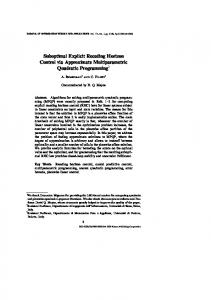
Figure 1: Tracking result of the explicit MPC with explicit MHE Problem (15) can be reformed as the following equivalent problem min ∆(k − N), . . . , ∆(k − 1) ¯ − N), . . . , ∆(k ¯ − 1) ∆(k

min x(k−N|k),..., ˆ x(k|k) ˆ

L(k)

and solved with the following design parameters.     100 0 0 0.01 0   0 0 0 ; Qy = R= ; 0 0.01 (17) 0 0 0

For fixed values of the Lagrange multipliers λ (k − N), . . . , λ (k − 1) and µ(k − N), . . . , µ(k), cost L(k) is a quadratic function of x(k ˆ − N|k), . . . , x(k|k), ˆ hence (17) is a quadratic problem which can be reformulated into mp-QP form. Then it can be solved by multi-parametric programming, resulting in an explicit robust moving horizon estimator.

5 Simulation results

N = 12;

Nc = 3.

We also designed a robust moving horizon estimator, considering both fast heating model and slow heating model simultaneously. Compared to MPC and standard MHE, robust MHE has much more parameters to optimize. So N should be chosen carefully. In this case we are using   100 0 Q= ; 0 100   10 0 0 0 ; R =  0 1000 0 0 0.1 N = 2.

After running the optimization routine over λ (k − Following the approach in Section 4.1, a robust MPC con- N), . . . , λ (k − 1), we set λ (k − N) = . . . = λ (k − 1) = troller is designed. A mixed integer program is formulated [21513, 21513].

24

Sui et.al., Robust Explicit MHC and MHE Tracking error 10 5 0

Temperature (K)

−5 −10 −15 −20 −25 −30 −35 −40

0

0.5

1

1.5

2

t (second)

2.5 4

x 10

Tracking error (zoomed in) 1

Temperature (K)

0.5

0

−0.5

−1

−1.5

−2

0

0.5

1

1.5 t (second)

2

2.5 4

x 10

Figure 2: Tracking error to the optimal temperature profile Applying the robust MPC and the robust MHE on the nonlinear polymerization reactor model described in Section 2.1, the following simulation results are obtained, shown in Figure 1 to Figure 3. Entry (1, 1) of Fig. 1 shows the temperature tracking ability, with red dashed line representing the optimal temperature reference, blue solid line the temperature output from the gPROMS model, and black dotted line the estimated temperature from MHE. The tracking error is depicted in Fig. 2, from which we can see that the maximum tracking error is about only 1.8K (the large tracking error around 22000 sec is because of the sudden change of optimal temperature profile, therefore is not considered). Entry (1, 2) and (1, 3) of Fig. 1 show the volume and pressure outputs from the gPROMS model and their estimates from MHE. The estimation error is given in Fig. 3 from which we can see that the estimation is accurate. Entry (2, 1) and (2, 2) of Fig. 1 gives weight/number average molecular weight (Mw and Mn ) and polydispersity and conversion rate. Entry (2, 3) of Fig. 1 gives the inputs, blue solid line for flow rate of cold water and green dashed line for the flow

rate of hot water. Comparing these figures with constraints listed in Table 2, it’s clear that all constraints are respected in this case study and the tracking performance is very good since the tracking error is quite small. Therefore it’s safe to say that the practical applicability of explicit MPC and MHE to a case with industrially relevant complexity has been proved.

6 Conclusion In this paper we proposed a combined robust model predictive control and robust moving horizon estimation approach for a batch polymerization process. Through multiparameter programming the most of the design work is accomplished off-line, leaving on-line only the job of evaluating the resulting PWA functions. Offset-free tracking and disturbance rejection ability are achieved. The simulation results demonstrate the effectiveness of the proposed approach.

25

Estimation error on temperature (K)

Modeling, Identification and Control 0.15 0.1 0.05 0 −0.05 −0.1 −0.15 −0.2

0

0.5

1

1.5

2

t (second)

2.5 4

x 10

Estimation error on volume (m3)

−4

5

x 10

0

−5

0

0.5

1

1.5

2

Estimation error on pressure (Pa)

t (second)

2.5 4

x 10

40

20

0

−20

−40

0

0.5

1

1.5 t (second)

2

2.5 4

x 10

Figure 3: Estimation error of the MHE

Acknowledgment

mance index. IEEE Transactions on Automatic Control, 2006. 51. doi:10.1109/TAC.2006.886486.

This work is supported by European project “Design of Advanced Controllers for Economic, Robust and Safe Manu- Bemporad, A., Borrelli, F., and Morari, M. Model predictive control based on linear programming-the explicit sofacturing Performance (CONNECT)". lution. IEEE Transactions on Automatic Control, 2002a. 47. doi:10.1109/TAC.2002.805688.

References

Bemporad, A. and Morari, M. Control of systems integrating logic, dynamics, and constraints. Automatica, 1999. Alessandri, A., Baglietto, M., and Battistelli, G. Robust 35(3):407–427. doi:10.1016/S0005-1098(98)00178-2. receding-horizon estimation for discrete-time linear systems in the presence of bounded uncertainties. Proceed- Bemporad, A., Morari, M., Dua, V., and Pistikopoulos, ings of the 44th IEEE Conference on Decision and ConE. N. The explicit linear quadratic regulator for control, 2005. pages 4269–4274. strained systems. Automatica, 2002b. 38(1):3–20. doi:10.1016/S0005-1098(01)00174-1. Asteasuain, M., Bandoni, A., Sarmoria, C., and Brandolin, A. Simultaneous process control design for Bonvin, D., Bodizs, L., and Srinivasan, B. Optimal grade transition in styrene polymerization. Chemgrade transition for polyethylene reactors via NCO trackical Engineering Science, 2006. 61:3362–3378. ing. Chemical Engineering Research and Design, 2005. doi:10.1016/j.ces.2005.12.012. 83(A6):692–697. doi:10.1205/cherd.04367. Baoti´c, M., Christophersen, F. J., and M., M. Constrained Brandrup, J., Immergut, E. H., and Grulke, E. A. Polymer optimal control of hybrid systems with a linear perforHandbook. Wiley, 4th edition, 2003.

26

Sui et.al., Robust Explicit MHC and MHE

Ferrari-Trecate, G., Mignone, D., and Morari, M. Moving horizon estimation for hybrid systems. IEEE Transactions on Automatic Control, 2002. 47. doi:10.1109/TAC.2002.802772. Grieder, P., Kvasnica, M., Baotic, M., and Morari, M. Stabilizing low complexity feedback control of constrained piecewise affine systems. Automatica, 2005. 41:1683– 1694. doi:10.1016/j.automatica.2005.04.016. Michalska, H. and Mayne, D. Q. Moving horizon observers. Nonlinear Control Systems Design Symp (NOLCOS), 1992. Morari, M. and Lee, J. H. Model predictive control: past, present and future. Computers and Chemical Engineering, 1999. 23:667–682. doi:10.1016/S00981354(98)00301-9. Pannocchia, G. and Bemporad, A. Combined design of disturbance model and observer for offset-free model predictive control. IEEE Transactions on Automatic Control, 2006. in press. doi:10.1109/TAC.2007.899096. Pannocchia, G. and Brambilla, A. How to use simplified dynamics in model predictive control of superfractionators. Industrial & Engineering Chemistry Research, 2005. 44(8):2687–2696. doi:10.1021/ie0495832. Russo, L. P. and Bequette, B. W. Process design for operability: A styrene polymerization application. Computers and Chemical Engineering, 1997. 21(6):571–576. Sayed, A. H., Nascimento, V. H., and Cipparrone, F. A. M. A regularized robust design criterion for uncertain data. SIAM Journal on Matrix Analysis and Applications, 2002. 23(4):1120–1142. doi:10.1137/S0895479800380799. Sui, D., Feng, L., and Hovd, M. Explicit moving horizon control and estimation: A batch polymerization case study. Industrial Electronics and Applications, 2009. pages 1656–1661. Torrisi, F. D. and Bemporad, A. HYSDEL—A tool for generating computational hybrid models. IEEE Transactions on Control System Technology, 2004. 12(2):235–249. doi:10.1109/TCST.2004.824309.

27