DCDIS A Supplement, Advances in Neural Networks, Vol. 14(S1) 536--542 Copyright@2007 Watam Press
Application of a Swarm-based Artificial Neural Network to Ultrasonic Detector Based Machine Condition Monitoring Shan He (
[email protected]), Xiaoli Li (
[email protected]), Cercia, School of Computer Science, The University of Birmingham, Birmingham, B15 2TT, UK
Abstract—Artificial Neural Networks (ANNs) have been applied to machine condition monitoring. This paper first addresses a ANN trained by Group Search Optimizer (GSO), which is a novel Swarm Intelligent (SI) optimization algorithm inspired by animal social foraging behaviour. The global search performance of GSO has been proven to be competitive to other evolutionary algorithms, such as Genetic Algorithms (GAs) and Particle Swarm Optimizer (PSO). Herein, the parameters of a 3-layer feed-forward ANN, including connection weights and bias are tuned by the GSO algorithm. Secondly the GSO based ANN is applied to model and analysis ultrasound data recorded from grinding machines to distinguish different conditions. The real experimental results show that the proposed method is capable to indicate the malfunction of machine condition from the ultrasound data.
Intelligent monitoring system
Machine
Index Terms—Ultrasonic, Condition Monitoring, Artificial Neural Networks, Swarm Intelligence, Evolutionary Algorithms
sensors and amplifiers
extraction of measured signal features
automatic feature selection
automatic feature integration
State of observed phenomenon
I. I NTRODUCTION Condition monitoring system is very important for some machinery, such as aircraft, and machine tool, and so on [1]. The main technologies of condition monitoring include sensors, signal processing and classification of condition [2]. A typical system is shown in Fig. 1. New techniques from computational intelligence have attracted the interest of condition monitoring system. These techniques include advance signal/data analysis, fuzzy logic, artificial neural networks, evolutionary computation and machine learning [1]. These computational techniques inspired by nature have shown promise in many condition monitoring system. Moving these techniques from simulated data sets, toy problems or laboratory settings to real industrial applications is still challenging [3]. Applications of ultrasonic detector for nondestructive testing are found in numerous industries, including refineries, pipe lines, power generation (nuclear or other), aircraft, offshore oil platforms, paper mills and structures (bridges, cranes, etc.). So far, the ultrasonic detector can solve the following problems in industrial practices: leak detection, crack detection, diagnostics and process monitoring.In order to apply for the ultrasonic detector for condition monitoring system, an advanced method should be developed to process the signals from the detector. Usually, an adaptive filter may be employed to the time series. Correspondence and requests for materials should be addressed to Dr. X. Li (email:
[email protected])
Fig. 1.
Intelligent condition monitoring system.
For instance, the adaptive LMS filter’s output is defined by the linear combination of the order statistics of the input samples in the filter window: Y (k) = aT (k)Xr (k) The coefficient vector a(k) is adapted at each step k accordingly to the LMS adaptation algorithm. The core of this filter is to build a simple model for the time series; then shifted series between the original series and the out of model, or socalled residue, is considered as noise. The noise information can be directly employed to diagnose the condition of machine [4]. It is noted a fact that machine faults often result from some sort of nonlinear operation of the machine involved, which may in turn lead to nonlinearities occurring in the machine’s signatures such as ultrasonic data [5]. A new signal processing techniques, such as neural network, can detect these nonlinearities. In particular, neural networks, fuzzy logic and evolutionary programming are widely applied to solve above complicated problems. In this study, ultrasonic detector is proposed to detect the malfunction of a machine. Ultrasonic detectors is made of piezo-electric quartz crystals. The detector can sense ultrasound generated from a machine. Ultrasound from mechanical 536
system is energy that created by the friction between moving components, such as bearings, gear mesh, etc. Therefore, the ultrasound is a reflection of machine condition. For example, the friction varies with the lubrication condition. Different friction leads different ultrasound, in turn, the ultrasound can be employed to predict the lubrication condition. Since 1980’s, the ultrasonic detectors have been applied for various maintenance of mechanical system. Previous work show that ultrasound-based condition monitoring is better than vibration. For instance, the low frequency vibration can indicate the wearing state of a bearing and provide information about root cause of premature failure. However, ultrasound can indicate necessary lubrication intervals, and triggers alarms before the bearing enters failure state. Ultrasound data is non-stationary, the traditional signal processing methods fail to build a suitable model to simulate it. In this paper, we will use a novel neural network trained by GSO to solve this problem. GSO is a novel SI algorithm for continuous optimization problems [6]. The algorithm is based on a generic social foraging model, Producer-Scrounger (PS) model, which is different from the metaphors used by the ACO and PSO. In order to evaluate its performance, extensive experimental study has been carried out. From the experimental results, it was found that the GSO algorithm has better search performance on large-scale multi-modal benchmark functions. Probably the most significant merits of GSO is that it provides an open framework to utilize research in animal behavioral ecology to tackle hard optimization problems. In this paper, the GSO algorithm is applied to ANN training to model ultrasound data for the condition monitoring. The rest of the paper is organized as follows. We present the background information of evolving ANNs, SI algorithms in Section II. The GSO algorithm and the GSO based ANN are introduced in Section III. In Section IV, the ultrasound data, experimental settings and the results will be given. The paper is concluded in Section V. II. B RIEF OVERVIEW OF A DVANCED A RTIFICIAL N EURAL N ETWORKS Artificial Neural networks (ANNs) are inspired by the workings of the human brain. They can be used as a universal function approximator, mapping an arbitrary number of inputs onto an arbitrary (but smaller) number of outputs (generally just one decision variable). This feature is particularly useful for modeling very complex systems. Essentially, neural networks model the process of the activation and strengthening of neural connections. Generally, they are built in layers comprising an input layer, an output layer and one or more hidden layers internally. Fig. 2 shows a very simple ANN model. Each neural connection is given a certain weight. These weights are then tuned on a training set by ANN training algorithms such that the ANN output most closely resembles the parameter that the network is designed to fit. The objective of ANN training algorithms is to minimize the least-square error between the desired output of the training set and the actual output of the ANN [7]
input layer
hidden layer output layer whn wkn f1 (¦ )
f1 (¦ )
yˆ1
xn
f h (¦ )
f k (¦ )
yˆ k
xN
f H (¦ )
f K (¦ )
yˆ K
x1
Th -1 Fig. 2.
bias
Tk -1
bias
A three-layer feed-forward ANN.
In this section, we loosely refer evolving artificial neural networks to those ANNs trained by Evolutionary Algorithms (EAs) and SI algorithms, such as PSO. Since the renaissance of ANNs in the 80s, EAs have been introduced to ANNs to perform various tasks, such as connection weight training, architecture design, learning rule adaption, input feature selection, connection weight initialization, rule extraction from ANN, etc. [8]. In [9], an improved genetic algorithm was used to tune the structure and parameters of a neural network. In order to tune the structure of ANN in a simple way, link switches were incorporated into a three layer neural network. By introducing link switches, a given fully connected feed-forward neural network may become a partially connected network after training [9]. An improved Genetic Algorithm (GA) with new genetic operators were introduced to train the proposed ANN. Two application examples, sunspots forecasting and associative memory tuning, were solved in their study. Palmes et al. proposed a mutation-based genetic neural network (MGNN) [10]. A simple matrix encoding scheme was used to represent an ANN’s architecture and weights. The neural network utilized a mutation strategy of local adaption of evolutionary programming to evolve network structures and connection weights dynamically. Three classification problems, namely iris classification, wine recognition problem, and Wisconsin breast cancer diagnosis problem were used in their paper as benchmark functions. In [11] a new type of EANN called memetic pareto artificial neural network (MPANN) was developed for breast cancer diagnosis. A multi-objective differential evolution algorithm was employed to determine the number of ANN’s hidden neurons and train its connection weights. In order to speed up the training process, a so-called memetic approach which combines the BP algorithm was used. Cant´u-Paz and Kamath presented an empirical evaluation of eight combinations of EAs and ANNs on 11 well studied real-world benchmaks and 4 synthetic problems [12]. The algorithms they used included binary-encoded, real-encoded GAs, and the BP algorithm. The tasks performed by these 537
algorithms and their combinations included searching for weights, designing architecture of ANNs, and selecting feature subsets for ANN training. SI algorithms have also been applied to ANN training. The expression “swarm intelligence” was coined by Beni and Wang in 1989 [13]. There is no commonly accepted definition of Swarm Intelligence (SI). As defined in [14]: SI is “an artificial intelligence technique based around the study of collective behavior in decentralized, self-organized systems.” According to [14] and also generally accepted by most of the researchers in SI, the most prominent components of SI are Ant Colony Optimiser (ACO) and Particle Swarm Optimiser (PSO), both of which are based on observations of collective animal behaviour. ACO is inspired by real ants’ foraging behaviour. In the ACO algorithm, artificial ants build solutions by moving on the problem graph and depositing artificial pheromone on the graph so that future artificial ants can build better solutions [14]. ACO has been successfully applied to a number of difficult optimization problems, e.g., traveling salesman problems. PSO is another well-known SI algorithm which glean ideas from animal aggregation behaviour. Artificial life models, such as BOID, which can mimic animal aggregation vividly, serve as the direct inspiration of PSO. The PSO algorithm is particularly attractive to practitioners because it has only a few parameters to adjust. In the past few years, the PSO algorithm has been successfully applied in many areas [15], [16]. In their seminal paper [17], Kennedy and Eberhart, who are the inventors of PSO, firstly applied PSO to train a simple multi-layer feedforward ANN to solve XOR problems. Since then, more and more SI algorithms including PSO and ACO have been applied to ANN training [18] [19]. III. G ROUP S EARCH O PTIMIZER BASED A RTIFICIAL N EURAL N ETWORKS
be calculated from ϕki via a Polar to Cartesian coordinates transformation:
dki1
=
n−1 Y
cos(ϕkip )
p=1
dkij
= sin(ϕki(j−1) ) ·
dkin
= sin(ϕki(n−1) )
n−1 Y
cos(ϕkip )
p=i
(1)
As same as the PS model, in the GSO, a group comprises producers and scroungers which perform producing and scrounging strategies, respectively. We also employ ‘rangers’ which perform random walks to avoid entrapment in local minima. For accuracy [21] and convenience of computation, in the GSO algorithm, we simplify the PS model by assuming that there is only one producer at each searching bout. This is based on the recent research [21], which suggested that the larger the group, the smaller the proportion of informed individuals need to guide the group with better accuracy. The simplest joining policy, which assumes all scroungers will join the resource found by the producer, is used. During each search bout, a group member, located in the most promising area, conferring the best fitness value, acts as the producer. It then stops and scans the environment to search resources (optima). Vision, as the main scanning mechanism used by many animal species [22], is employed by the producer in GSO. In order to handle optimization problems of whose number of dimensions usually is larger than 3, the scanning field of vision is generalized to a n dimensional space, which is characterized by maximum pursuit angle θmax ∈ Rn−1 and maximum pursuit distance lmax ∈ R1 as illustrated in a 3D space in Figure 3. In the GSO algorithm, at the kth iteration the producer Xp behaves as follows:
A. Group Search Optimizer The Group Search Optimizer is a novel swarm intelligence algorithm inspired by animal social foraging behavior [6]. The GSO algorithm employs the Producer-Scrounger (PS) model [20] as a framework. The PS model was firstly proposed by C.J. Barnard to analyze social foraging strategies of group living animals. In this model, it is assumed that there are two foraging strategies within groups: (1) producing, e.g., searching for food; and (2) joining (scrounging), e.g., joining resources uncovered by others. Foragers are assumed to use producing or joining strategies exclusively. Under this framework, concepts of resource searching from animal scanning mechanism are used to design optimum searching strategies to design the GSO algorithm. Basically, GSO is a population based optimization algorithm. The population of the GSO algorithm is called a group and each individual in the population is called a member. In an n-dimensional search space, the ith member at the kth searching bout (iteration), has a current position Xik ∈ Rn , a head angle ϕki = (ϕki1 , . . . , ϕki(n−1) ) ∈ Rn−1 and a head direction Dik (ϕki ) = (dki1 , . . . , dkin ) ∈ Rn which can
M a x im
r s u it um pu
a n g le
θ max 0o
Maximumpursuitangle
M ax im um
Fig. 3.
pu rs ui t di st
θ max
(For w ard dire cted )
an ce l m ax
Scanning field in 3D space [22]
1) The producer will scan at zero degree and then scan laterally by randomly sampling three points in the scanning field [23]: one point at zero degree: Xz = Xpk + r1 lmax Dpk (ϕk )
(2)
one point in the right hand side hypercube: Xr = Xpk + r1 lmax Dpk (ϕk + r2 θmax /2)
(3)
and one point in the left hand side hypercube: Xl = Xpk + r1 lmax Dpk (ϕk − r2 θmax /2)
(4) 538
where r1 ∈ R1 is a normally distributed random number with mean 0 and standard deviation 1 and r2 ∈ Rn−1 is a random sequence in the range (0, 1). 2) The producer will then find the best point with the best resource (fitness value). If the best point has a better resource than its current position, then it will fly to this point. Otherwise it will stay in its current position and turn its head to a new angle: ϕk+1 = ϕk + r2 αmax
(5)
where αmax is the maximum turning angle. 3) If the producer cannot find a better area after a iterations, it will turn its head back to zero degree: ϕk+a = ϕk
(6) √ where a is a constant given by round( n + 1). At each iteration, a number of group members are selected as scroungers, which keep searching for opportunities to join the resources found by the producer. The commonest scrounging behavior [20] in house sparrows (Passer domesticus): area copying, that is, moving across to search in the immediate area around the producer, is adopted. At the kth iteration, the area copying behavior of the ith scrounger can be modeled as a random walk towards the producer: Xik+1 = Xik + r3 (Xpk − Xik )
(7)
where r3 ∈ Rn is a uniform random sequence in the range (0, 1). In group-living animals, group members often have different searching and competitive abilities; subordinates, who are less efficient foragers than the dominant will be dispersed from the group [24]. This may result in ranging behavior, which is an initial phase of a search that starts without cues leading to a specific resource [25]. In our GSO algorithm, rangers are introduced to explore a new search space therefore to avoid entrapments of local minima. Random walks, which are thought to be the most efficient searching method for randomly distributed resources [26], are employed by rangers. If the ith group member is selected as a ranger, at the kth iteration, it generates a random head angle ϕi : ϕk+1 = ϕki + r2 αmax i
(8)
where αmax is the maximum turning angle; and it chooses a random distance: li = a · r1 lmax
(9)
and move to the new point: Xik+1 = Xik + li Dik (ϕk+1 )
(10)
In order to maximize their chances of finding resources, animals restrict their search to a profitable patch. One strategy is turning back into a patch when its edge is detected [27]. This strategy is employed by GSO to handle the bounded search space: when a member is outside the search space, it will turn back to its previous position inside the search space.
B. Training Artificial Neural Networks using GSO The ANN weight training problem is essentially a hard continuous optimization problem because the search space is high-dimensional multi-modal and is usually polluted by noises and missing data. Therefore, it is quite logically to apply our GSO algorithm to ANN weight training. The objective of ANN weight training process is to minimize an ANN’s error function. However, it has been pointed out that minimizing the error function is different from maximizing generalization [28]. Therefore, to improve ANN’s generalization performance, in this study, an early stopping scheme is introduced. The error rates of validation sets are monitored during the training processes. When the validation error increases for a specified number of iterations, the training will stop. In this study, the GSO algorithm and early stopping scheme have been applied to training an ANN. In this study, the ANN we employed consists three layers, namely, input, hidden, and output layers. The nodes in each layer receive input signals from the previous layer and pass the output to the subsequent layer. The nodes of the input layer supply respective elements of the activation pattern (input vector), which constitute the input signals from outside system applied to the nodes in the hidden layer by the weighted links. The output signals of the nodes in the output layer of the network constitute the overall response of the network to the activation pattern supplied by the source nodes in the input layer [7]. The subscripts n, h, and k denote any node in the input, hidden, and output layers, respectively. The net input u is defined as the weighted sum of the incoming signal minus a bias term. The net input of node h , uh , in the hidden layer is expressed as follows: uh =
n X
whn yn − θh
where yn is the output of node n in the input layer, whn represents the connection weight from node n in the input layer to node h in the hidden layer, and θh is the bias of node h in the hidden layer. The activation function used in the proposed ANN is the sigmoid function. Therefore, in the hidden layer, the output yh of node h, can be expressed as yh = fh (uh ) =
1 1 + euh
The output of node k in the output layer can be also described as: 1 (11) yk = fk (uk ) = 1 + euk where X uk = wkh yh − θk h
where θk is the bias of node k in the output layer. The parameters (connection weights and bias terms) are tuned by the GSO algorithm. In the GSO-based training algorithm, each member of the population is a vector comprising connection weights and bias terms. Without loss of generality, we denote W1 as the connection weight matrix between the input layer and the hidden layer, Θ1 as the bias terms to 539
DesiredOutput
Input
input layer
ANNOutput
hidden layer
y(t-1)
f1 ( å )
y(t-h)
f h (å )
output layer
ANN Error
AjustParameters Fig. 4.
f k (å )
yˆ (t )
GSO
Schematic diagram of GSO based ANN.
f H (å )
y(t-l)
the hidden layer, W2 as the one between the hidden layer and the output layer, and Θ2 as the bias terms to the output layer. The ith member in the population can be represented as: Xi = [W1i Θi1 W2i Θi2 ]. The fitness function assigned to the ith individual is the least-squared error function defined as follows: Fi =
P X K X
1 2 p=1
i 2 (dkp − ykp )
q -1 Fig. 5.
h
bias
ANN for time series modeling.
(12) ANN model 1 Input
. . .
ANN model n . . .
ANN model N
IV. A PPLICATION OF GSOANN
-1
Measured ultrasound
k=1
i indicates the kth computed output in equation (11) where ykp of the ANN for the pth sample vector of the ith member; P denotes the total number of sample vectors; and dkp is the desired output in the kth output node.
q k bias
-
Residual
-
Classifier
-
TO ULTRASONIC
DETECTOR
Fig. 6.
The structure of the model-based condition monitoring system.
A. Ultrasound Modeling with GSOANN Ultrasound is a time-series that is generated by a dynamic system such as a running machine. In fact, the ultrasound is an output of this dynamic system. A simple idea is to build a model for this dynamic system by using this output. Traditional methods are to make use of the series relation at past and current conditions for modelling the dynamical system. Herein, we will apply GSOANN to build a model for ultrasound from a griding machine tool. Denote a ultrasound series at instant t as y(t), where y may be a vector, then the time series model can be described as y(t) = f (t − 1, t − 2, · · · t − l), where f (·) is a modeling function. Once the model is constructed, it can be used for further analysis, e.g., forecasting, control, and diagnosis. In the past few decades, ANNs has attracted more and more attention since they provide an powerful alternative to model a complex dynamical system. The ANN time series modeling can be described as N N (t − 1, t − 2, · · · t − l), where N N (·) stand for a neural network modeler. In this study, an ANN model based condition monitoring system is proposed, as illustrated in Fig. 6. To make use of this system to identify the condition of a machine, it is necessary to record ultrasound data at different conditions, including normal and abnormal states. Then using the measured ultrasound as input to the trained ANN models, we can obtain the expected outputs, the differences between the actual ultrasound data and expected outputs from the ANN
models can be calculated to form the residuals. The residual then may be used to indicate the different conditions of the machine. Each case will have different residuals, the smaller the residual, the closer to to the state of the compared ANN model. For a complex condition monitoring system, a classifier will be used to distinguish different states. B. Case study: Condition Monitoring in Grinding In this study, we use the GSOANN to build time series models of ultrasound in grinding to identify the condition of a machine. Fig. 7 shows the measurement of sound signal from a grinding machine. The sound is recorded by a ultrasonic detector nearby the motor. The data was recorded using 44100 Hz sampling rate with 16 bits per sample, then the data is saved/transferred to a computer for further analysis. In the meanwhile, we also measure different positions, because of the difference of structure, the ultrasound is different. We have recorded two types of ultrasound data, one is normal condition, another is abnormal. Firstly we aim to model these two ultrasound data sets using GSOANN. Then we will investigate whether the GSOANN models can be used to distinguish healthy/faulty conditions from unknow ultrasound. Fig. 8 and 9 show the ultrasound sample of normal and abnormal condition, respectively. The total length of the sound sample from normal and abnormal conditions are 9.6632 and 540
Amp.
0.05
0
−0.05 0
Fig. 9.
1
2
3
4 5 Time Sec.
6
7
8
9
Ultrasound data sample from a machine in normal condition.
0.2 ANN output ultrasound data
0.15
Amp.
0.1
Fig. 7.
The measurement of ultrasound data from the grinding machine.
0.05 0 -0.05 -0.1
0.2
-0.15 0.8
0.15 0.1
Amp.
0.82 0.83 Time Sec.
0.84
0.85
Fig. 10. Testing results from ANN ultrasound model of the machine in abnormal condition in comparison with the actual unseen ultrasound data. Ultrasound fragment taken from 0.8-0.85 second
0.05 0 −0.05 −0.1 −0.15 −0.2 0
Fig. 8.
0.81
1
2
3
4 5 Time Sec.
6
7
8
Ultrasound data sample from a machine in abnormal condition.
8.1422 seconds, respectively. We use the first 5 seconds data of these samples as ANN training sets to construct ultrasound models. To build a model for ultrasound data, a 3-layer feedforward neural network with 4 hidden neurons is employed. The training algorithm we chose is the GSO based training algorithm in Section III. To reduce the complexity of the ANN, we only select six past data points as the inputs: x(t − 0.01), x(t − 0.02), x(t − 0.03), x(t − 0.04), x(t − 0.05), x(t − 0.06); the output is x(t). The input and output are normalized so that they fall in the interval [−1, 1]. The number of epoch for
training is set to be 150. Once the models are constructed, we then can test the condition of the machine by using unknown ultrasound data. We select a ultrasound data of 3.1422 seconds recorded from machine at normal condition for testing. The data will be input into two constructed models. The errors between model output and actual ultrasound will be calculated to form the residues. We select a ultrasound of 0.03 second to illustrate the details of the GSOANN model output in comparison with the actual data, as shown in Fig. 10. The error rate between output of GSOANN model at abnormal condition and actual ultrasound data is 0.0024%. The output of the GSOANN model at normal condition is shown in Fig. 11. It can be seen that, the difference between model output and actual ultrasound is large. The error rate calculated from GSOANN output is 0.008%, which is almost 4 times larger than the error rate obtained by the GSOANN model at abnormal condition. V. C ONCLUSION In this study, we proposed an novel ANN trained by a SI algorithm GSO, GSOANN for machine condition monitoring. 541
0.05
Amp.
Ultrasound EANN output
0
-0.05 0
1
2 3 Time Sec.
4
5
0.05
Amp.
Ultrasound EANN output
0
-0.05 0.18
0.2 Time Sec.
Fig. 11. Testing results from ANN ultrasound model of the machine at normal condition in comparison with the actual unseen ultrasound data. Ultrasound fragment taken from 0.18-0.2 second
We have successfully constructed GSOANN models for ultrasound data to monitor the machine conditions in grinding. Based on the case study, it is found that the proposed method is capable to approximate the ultrasound data of different conditions. Preliminary experiments show that these models can be used to indicate the condition from ultrasound recorded. However, it would be more helpful to expend the classification to other conditions, such as lubrication conditions. Therefore, to assure and widen the applicability of the proposed method, more experiments are required. R EFERENCES [1] X Li, Y. Yao, and Yuan Z. On-line tool condition monitoring using wavelet fuzzy neural network. Journal of Intelligent Manufacturing, 8:271–276, 1997. [2] X Li, , Y. Ou, X. P. Guan, and R. Du. Ram velocity control in plastic injection molding machines with higher order iterative learning. Control and Intelligent Systems, 34:64–71, 2006. [3] X. Li, R. Du, B. Denkena, and J. Imiela. Tool breakage monitoring using motor current signals for machine tools with linear motors. IEEE Trans. Industrial Electronic, 52:1403–1409, 2005. [4] X. Li and R. Du. Condition monitoring using latent process model with an application to sheet metal stamping processes. ASME Trans. J. Manuf. Sci. Engg., 127:376–385, 2005. [5] X. Li. Detection of tool flute breakage in end milling using feed-motor current signatures. IEEE/ASME Transactions on Mechatronics, 6:376– 385, 2001.
[6] S. He, Q. H. Wu, and J. R. Saunders. A novel group search optimizer inspired by animal behavioural ecology. In 2006 IEEE Congress on Evolutionary Computation (CEC 2006), pages Tue PM–10–6, Sheraton Vancouver Wall Centre, Vancouver, BC, Canada., July 2006. [7] S. Haykin. Neural Networks. A Comprehensive Foundation. Prentice Hall, New Jersey, USA, 1999. [8] X. Yao. Evolving artificial neural networks. Proceeding of the IEEE, 87(9):1423–1447, Sep. 1999. [9] F. H. F. Leung, H. K. Lam, S. H. Ling, and P. K. S. Tam. Tuning of the structure and parameters of a neural network using an improved genetic algorithm. IEEE Trans. on Neural Networks, 14(1):79–88, Jan. 2003. [10] P. P. Palmes, T. Hayasaka, and S. Usui. Mutation-based genetic neural network. IEEE Trans. on Neural Networks, 16(3):587–600, MAY 2005. [11] H. A. Abbass. An evolutionary artificial neural networks approach for breast cancer diagnosis. ARTIFICIAL INTELLIGENCE IN MEDICINE, 25:265–281, 2002. [12] E. Cantu-Paz and C. Kamath. An empirical comparison of combinations of evolutionary algorithms and neural networks for classification problems. IEEE Transactions on Systems, Man, and Cybernetics-Part B: Cybernetics, 35(5):915–927, 2005. [13] G. Beni and J. Wang. Swarm intelligence. In Seventh Annual Meeting of the Robotics Society of Japan, pages 425–428, Tokio, Japan, 1989. RSJ press. [14] Wikipedia. Swarm intelligence — wikipedia, the free encyclopedia, 2005. [Online; accessed 21-JULY-2006]. [15] S. He, J. Y. Wen, E. Prempain, Q. H. Wu, J. Fitch, and S. Mann. An improved particle swarm optimization for optimal power flow. In 2004 International Conference on Power System Technology, Nov. 2004. [16] S. He, E. Prempain, and Q. H. Wu. An improved particle swarm optimizer for mechanical design optimization problems. Engineering Optimization, 36(5):585–605, Oct. 2004. [17] J. Kennedy and R.C. Eberhart. Particle swarm optimization. In IEEE international Conference on Neural Networks, volume 4, pages 1942– 1948. IEEE Press, 1995. [18] Christian Blum and Krzysztof Socha. Training feed-forward neural networks with ant colony optimization: An application to pattern classification. In HIS ’05: Proceedings of the Fifth International Conference on Hybrid Intelligent Systems, pages 233–238, Washington, DC, USA, 2005. IEEE Computer Society. [19] F. van den Bergh and A. Engelbrecht. Cooperative learning in neural networks using particle swarm optimizers. South African Computer Journal, 26:84–90, 2000. [20] C. J. Barnard and R. M. Sibly. Producers and scroungers: a general model and its application to captive flocks of house sparrows. Animal Behaviour, 29:543–550, 1981. [21] I.D. Couzin, J. Krause, N.R. Franks, and S.A. Levin. Effective leadership and decision-making in animal groups on the move. Nature, 434:513– 516, Feb. 2005. [22] J. W. Bell. Searching Behaviour - The Behavioural Ecology of Finding Resources. Chapman and Hall Animal Behaviour Series. Chapman and Hall, 1990. [23] W. J. O’Brien, B. I. Evans, and G. L. Howick. A new view of the predation cycle of a planktivorous fish, white crappie (pomoxis annularis). Can. J. Fish. Aquat. Sci., 43:1894–1899, 1986. [24] D. G. C. Harper. Competitive foraging in mallards: ’ideal free’ ducks. Animal Behaviour, 30:575–584, 1988. [25] D. B. Dusenbery. Ranging strategies. Journal of Theoretical Biology, 136:309–316, 1989. [26] G. M. Viswanathan, S. V. Buldyrev, S. Havlin, M. G. da Luz, E. Raposo, and H. E. Stanley. Optimizing the success of random searches. Nature, 401(911-914), 1999. [27] A. F. G. Dixon. An experimental study of the searching behaviour of the predatory coccinellid beetle adalia decempunctata. J. Anim. Ecol., 28:259–281, 1959. [28] D. H. Wolpert. A mathematical theory of generalization. Complex Systems, 4(2):151–249, 1990.
542